Empirical Means on Pseudo-Orthogonal Groups

Abstract

The present article studies the problem of computing empirical means on pseudo-orthogonal groups. To design numerical algorithms to compute empirical means, the pseudo-orthogonal group is endowed with a pseudo-Riemannian metric that affords the computation of the exponential map in closed forms. The distance between two pseudo-orthogonal matrices, which is an essential ingredient, is computed by both the Frobenius norm and the geodesic distance. The empirical-mean computation problem is solved via a pseudo-Riemannian-gradient-stepping algorithm. Several numerical tests are conducted to illustrate the numerical behavior of the devised algorithm.

1. Introduction

The present article aims at investigating a least-squares problem on the pseudo-orthogonal Lie group $O(p,q)$ (we follow the nomenclature in [1]) endowed with a pseudo-Riemannian metric that affords the computation of geodesic in closed form, with the aim of computing the empirical mean value $\mu$ of a finite collection of pseudo-orthogonal matrices. The empirical mean value $\mu$ of a distribution of points on a manifold is instrumental in several applications (see, for example, the article [2] that concerns the statistics of covariance matrices for biomedical engineering applications, the article [3] that deals with urban mobility analysis and the article [4] that concerns water quality assessment). The mean value $\mu$ is, by definition, close to all points in the distribution and this makes the tangent space at $\mu$ a good candidate as a reference space for numerical calculations (see, for example, [5]) as well as empirical statistical evaluations (see, for example, [6] and, for a recent account, [7]).

Since, in general, an empirical mean of a collection of mathematical objects living in a metric space is the closest point in the space to all points in the collection, the problem of defining and computing an empirical mean may be formulated in terms of minimization of a sum-of-squared distance problem. Function minimization over smooth matrix manifolds has received considerable attention due to its broad application range [8,9,10,11,12,13]. In general, smooth manifolds in function optimization serve to conveniently represent non-linear constraints. Constrained optimization arises in several branches of science, ranging from applied mathematics [14,15,16] to information sciences [14,17,18]. In [19,20], optimization-based mean-computation problems over the space of the symmetric positive-definite matrices, the special Euclidean group and the space of unipotent matrices were studied. The authors of [21] investigated the problem of computing empirical arithmetic averages over the Stiefel manifolds by tangent-bundle maps. Similarly, in [22], the authors studied empirical arithmetic-mean computation algorithms over the Grassmann manifolds. In [23], the author studied non-compact matrix-type manifolds (for example, the real symplectic group).

A special case of pseudo-orthogonal group is the Lorentz group $O(1,3)$, which describes Lorentz transformations of Minkowski space-time, the classical setting for non-gravitational physical phenomena. Lorentz groups are likewise relevant in classical ray optics [24]. Moreover, the Lorentz group is related with Poincaré groups, which may be seen as the semidirect product of Lorentz and translation groups [25]. In engineering, the Lorentz group plays a fundamental role, e.g., in the analysis of motion of charged particles in electromagnetism. For instance, the article [26] investigates on the computation of the trajectory of a charged particle in a magnetic field (such as an electron trapped in a cusp-shaped magnetic field) in terms of the Lorentz-group’s Lie-algebra map.

The present article is organized as follows. Section 2 recalls some fundamental notions on the geometry of pseudo-Riemannian manifolds and the gradient-steepest-descent function-minimization method on pseudo-Riemannian manifolds. The present article takes the route of embedding a pseudo-orthogonal group $O(p,q)$ into the Euclidean ambient space ${\mathbb{R}}^{(p+q)\times (p+q)}$ and to formulate all equations without recurring to any specific coordinate system nor any specific base for the associated tangent bundle. Section 3 introduces the pseudo-Riemannian geometric structure of the pseudo-orthogonal group and presents the necessary calculations to tackle function-minimization problems over such matrix group. Section 4 presents results of several numerical tests about computing a mean matrix over a pseudo-orthogonal group. Section 5 concludes the article.

2. Function Minimization on Pseudo-Riemannian Smooth Manifolds

For a certain pseudo-Riemannian manifold M endowed with a distance function $d(·,·)$, the empirical mean $\mu \in M$ of a finite collection of points $x_1,x_2\cdots x_N\in M$ is defined as

$$\mu :=arg\underset{x\in M}{min}\sum _k{d}^2(x,x_k).$$

(1)

In the present section, we summarize the notion of function minimization over a smooth pseudo-Riemannian manifold from previous research endeavors. Section 2.1 recalls fundamental notions from differential geometry, while Section 2.2 summarizes the main ideas behind pseudo-gradient-based function minimization on pseudo-Riemannian manifolds.

2.1. Notes on Pseudo-Riemannian Manifolds

Let M denote a p-dimensional pseudo-Riemannian submanifold of the general linear group and let $T_{x}M$ denote the tangent space of M at the point x. The symbol $TM:=\{(x,v)\mid x\in M,v\in T_{x}M\}$ denotes the tangent bundle associated to the manifold M and the symbol $\mathsf{\Gamma }(TM)$ denotes the set of vector fields on M. The cotangent space of M at a point x is denoted by $T_x^{*}M$. We denote by the symbol ${\langle ·,·\rangle }^{\mathrm{E}}$ the Euclidean inner product.

A pseudo-Riemannian manifold is endowed with an indefinite inner product ${\langle ·,·\rangle }_x:T_{x}M\times T_{x}M\to \mathbb{R}$, $x\in M$. An indefinite inner product is a non-degenerate, smooth, symmetric, bilinear map which assigns a real number to pairs of tangent vectors at each tangent space of a manifold. In pseudo-Riemannian geometry, the metric tensor is symmetric and invertible but not necessarily positive-definite.

Let $f:M\to \mathbb{R}$ denote a differentiable function. The differential of a function $f:M\to \mathbb{R}$ at a point $x\in M$ is denoted by $d{f}_x\in T_x^{*}M$ and satisfies the relationship $d{f}_x(v)={\langle {\nabla }_{x}f,v\rangle }_x,$ where ${\nabla }_{x}f\in T_{x}M$ denotes the pseudo-Riemannian gradient. Once a metric is selected, the pseudo-Riemannian gradient of a smooth function can be computed by the condition ${\langle {\partial }_{x}f,v\rangle }^{\mathrm{E}}={\langle {\nabla }_{x}f,v\rangle }_x,\forall v\in T_{x}M.$

The covariant derivative of a vector field $v\in \mathsf{\Gamma }(TM)$ in the direction of a tangent vector $w\in T_{x}M$ is denoted as ${\nabla }_{w}v$. In the present article, the notion of connection refers to a Levi–Civita connection. The calculation of the expression of geodesics associated to a given metric on a pseudo-Riemannian manifold may be formulated in variational terms as recalled in the following

Lemma 1

([23]). Let $\gamma :[0,1]\to M$ be a sufficiently regular curve with fixed endpoints, then the geodesic equation ${\nabla }_{\dot{\gamma }}\dot{\gamma }=0$ is equivalent to the equation

$$\delta {\int }_0^1{\langle \dot{\gamma },\dot{\gamma }\rangle }_{\gamma }dt=0,$$

(2)

where δ denotes the variation of the integral functional. Namely, γ satisfies the geodesic equation if and only if it is a critical point of the energy functional (define on the space of $C^1$-paths with fixed endpoints).

This is, indeed, a well-known result: although the metric is pseudo-Riemannian, its proof is the same as in the Riemannian case where there exist several references (see, e.g., [27]).

The variational formulation to compute the explicit expression of geodesics in embedded manifolds is easier to use in practical calculations than the covariant-derivative-based definition.

2.2. Gradient-Based Function Minimization on Pseudo-Riemannian Manifolds

On a geodesically complete Riemannian manifold M, the metric is positive definite, hence the squared geodesic distance connecting two points $x_1,x_2\in M$ is defined as

$$d^2(x_1,x_2):={\left({\int }_0^1\sqrt{{\langle \dot{\gamma },\dot{\gamma }\rangle }_{\gamma }}dt\right)}^2={\langle \dot{\gamma },\dot{\gamma }\rangle }_{\gamma }{|}_{t=0}.$$

(3)

If the geodesic is denoted as ${\gamma }_{x,v}(t)$, which indicates that the geodesic arc is departing from the point $x\in M$ with initial direction $v\in T_{x}M$, then the squared geodesic distance equals ${\parallel v\parallel }_x^2$.

When the Riemannian manifold of interest M and a regular criterion function $f:M\to \mathbb{R}$ are specified, a geodesic-based Riemannian-gradient-steepest-descent function-minimization method is expressed as

$$x_{(\ell +1)}={\gamma }_{x_{(\ell )},-{\nabla }_{x_{(\ell )}}f}(t_{(\ell )}),\mathrm{with}{t}_{(\ell +1)}=arg\underset{t>0}{min}\{f({\gamma }_{x_{(\ell )},-{\nabla }_{x_{(\ell )}}f}(t))\},$$

(4)

where $\ell \ge 0$ denotes an iteration step-counter, $t_{(\ell )}$ denotes a step-size schedule and the initial guess $x_{(0)}\in M$ is arbitrarily chosen.

Since a pseudo-Riemannian manifold is a manifold endowed with a metric that is not necessarily positive-definite, on a pseudo-Riemannian manifold M, the quantity ${\parallel v\parallel }_x^2$ may be positive, negative or null even for $0\ne v\in T_{x}M$. A key step in pseudo-Riemannian geometry is to decompose each tangent space $T_{x}M$ as

$$\left\{\begin{array}{c}{T}_x^{+}M:=\{v\in T_x{M|\parallel v\parallel }_x^2>0\},\\ T_x^{0}M:=\{v\in T_x{M|\parallel v\parallel }_x^2=0\},\\ T_x^{-}M:=\{v\in T_x{M|\parallel v\parallel }_x^2<0\}.\end{array}\right.$$

(5)

Given a pseudo-Riemannian manifold M and a regular criterion function $f:M\to \mathbb{R}$, a “gradient steepest descent” function minimization rule is expressed as

$$\dot{x}=\left\{\begin{array}{cc}-{\nabla }_{x}f,\hfill & \mathrm{if}{\nabla }_{x}f\in T_x^{+}M\cup T_x^{0}M,\hfill \\ {\nabla }_{x}f,\hfill & \mathrm{if}{\nabla }_{x}f\in T_x^{-}M,\hfill \end{array}\right.$$

(6)

which can be implemented numerically by a geodesic-based stepping method which moves a point along a short self-parallel arc in the direction of the pseudo-Riemannian gradient

$$x_{(\ell +1)}=\left\{\begin{array}{cc}{\gamma }_{x_{(\ell )},-{\nabla }_{x_{(\ell )}}f}(t_{(\ell )}),\hfill & \mathrm{if}{\nabla }_{x_{(\ell )}}f\in T_{x_{(\ell )}}^{+}M\cup T_{x_{(\ell )}}^{0}M,\hfill \\ {\gamma }_{x_{(\ell )},{\nabla }_{x_{(\ell )}}f}(t_{(\ell )}),\hfill & \mathrm{if}{\nabla }_{x_{(\ell )}}f\in T_{x_{(\ell )}}^{-}M.\hfill \end{array}\right.$$

(7)

The step-size schedule $t_{(\ell )}$ may be defined on the basis of an optimality condition, which resembles Armijo’s line search method [28], under the assumption that ${\nabla }_{x_{(\ell )}}f\notin T_{x_{(\ell )}}^{0}M$ (see [23]). Define the function

$${\tilde{f}}_{(\ell )}:=f\circ {\gamma }_{x_{(\ell )},v_{(\ell )}}(t):{\mathbb{R}}_{+}\to \mathbb{R},$$

(8)

where $v_{(\ell )}=-{\nabla }_{x_{(\ell )}}f$, if ${\nabla }_{x_{(\ell )}}f\in T_{x_{(\ell )}}^{+}M$, while $v_{(\ell )}={\nabla }_{x_{(\ell )}}f$, if ${\nabla }_{x_{(\ell )}}f\in T_{x_{(\ell )}}^{-}M$. The value ${\tilde{f}}_{(\ell )}(0)-{\tilde{f}}_{(\ell )}(t)\ge 0$ denotes the decrease of the criterion function f subject to a pseudo-geodesic step of size t. If the value of the geodesic step-size t is small enough, such decrease can be expanded in Taylor series as

$${\tilde{f}}_{(\ell )}(0)-{\tilde{f}}_{(\ell )}(t)=-{\tilde{f}}_{1(\ell )}t-\frac{1}{2}{\tilde{f}}_{2(\ell )}{t}^2+o(t^2),$$

(9)

where the coefficients ${\tilde{f}}_{1(\ell )},{\tilde{f}}_{2(\ell )}$ of the Taylor expansion are defined as

$${\tilde{f}}_{1(\ell )}=\frac{d{\tilde{f}}_{(\ell )}}{dt}{|}_{t=0},{\tilde{f}}_{2(\ell )}=\frac{d^2{\tilde{f}}_{(\ell )}}{d{t}^2}{|}_{t=0}.$$

(10)

Under such second-order Taylor approximation, the step-size value that maximizes the decrease rate is

$$t_{(\ell )}:=arg\underset{t}{max}(-{\tilde{f}}_{1(\ell )}t-\frac{1}{2}{\tilde{f}}_{2(\ell )}{t}^2)=-{\tilde{f}}_{1(\ell )}{\tilde{f}}_{2(\ell )}^{-1}.$$

(11)

The above choice for the step-size schedule is optimal only if ${\tilde{f}}_{1(\ell )}\le 0$, ${\tilde{f}}_{2(\ell )}>0$, because these two conditions ensure that $t_{(\ell )}\ge 0$, hence that the algorithm is always seeking for the minimum of the criterion function f.

Given a precision value $ϵ>0$ and under the assumption that ${\nabla }_{x}f\notin T_x^{0}M$, the numerical procedure stops at step $\overline{\ell }$ if

$$-{\tilde{f}}_{1(\overline{\ell })}<ϵ.$$

(12)

This condition expresses the fact that the value taken by the first derivative of the function $\tilde{f}$ is so small that no further improvements can be gained by continuing with the iteration. For the sake of consistency, it is assumed that the function f be bounded from below in M.

3. Function Minimization on the Pseudo-Orthogonal Group

Two criterion functions on the pseudo-orthogonal group that encode the notion of average squared distance may be constructed on the basis of the Frobenius norm and of the induced geodesic distance on the pseudo-orthogonal group $O(p,q)$. The related function minimization problem can be solved numerically by a pseudo-Riemannian-gradient-based algorithm.

In the present section, we deal with a matrix manifold, therefore it pays to recall that, on a matrix space, ${\langle A,B\rangle }^{\mathrm{E}}:=\mathrm{tr}(A^{\top }B)$, where ${}^{\top }$ denotes matrix transpose and “$\mathrm{tr}$” denotes a matrix trace operator. The matrix Frobenius norm is defined by ${\parallel A\parallel }_{\mathrm{F}}:=\sqrt{{\langle A,A\rangle }^{\mathrm{E}}}$.

Section 3.1 surveys the geometric structure of the pseudo-orthogonal group and describes a pseudo-Riemannian metrization. Section 3.2 and Section 3.3 describe two different criterion functions to compute the geodesic mean over a pseudo-orthogonal group and present the related numerical function minimization algorithms.

3.1. Pseudo-Riemannian Geometric Structure of the Pseudo-Orthogonal Group

A pseudo-orthogonal group $O(p,q)$, as a non-compact matrix Lie group [29], is an instance of quadratic groups and is defined by

$$O(p,q):=\{X\in {\mathbb{R}}^{(p+q)\times (p+q)}\mid X^{\top }{R}_{p,q}X=R_{p,q}\},R_{p,q}:=\left(\begin{array}{cc}{I}_p& O_{p\times q}\\ O_{q\times p}& -I_q\end{array}\right),$$

(13)

where the symbol $I_p$ denotes a $p\times p$ identity matrix and the symbol $O_{p\times q}$ denotes a whole-zero $p\times q$ matrix. The matrix $R_{p,q}$ enjoys the properties $R_{p,q}^2=I_{p+q},R_{p,q}^{\top }=R_{p,q}^{-1}=R_{p,q}$. Pseudo-orthogonal matrices enjoy two properties that are recalled in the following.

Lemma 2.

Any pseudo-orthogonal matrix $X\in O(p,q)$ is invertible. In addition, it holds that ${\parallel X\parallel }_{\mathrm{F}}={\parallel X^{-1}\parallel }_{\mathrm{F}}$.

Proof. 

From the defining property $X^{\top }{R}_{p,q}X=R_{p,q}$, it follows that $det(X^{\top }{R}_{p,q}X)=det(R_{p,q})$, hence $det{(X)}^2=1$, which proves the first assertion. From the definition of pseudo-orthogonal matrices, there follow the identities

$$X^{\top }=R_{p,q}{X}^{-1}{R}_{p,q},X^{-\top }=R_{p,q}X{R}_{p,q},$$

(14)

which are often useful in the course of calculations. By the first identity in Equation (14), it is easy to see that

$${\parallel X\parallel }_{\mathrm{F}}=\mathrm{tr}(X{X}^{\top })=\mathrm{tr}(X{R}_{p,q}{X}^{-1}{R}_{p,q})=\mathrm{tr}(R_{p,q}X{R}_{p,q}{X}^{-1}),$$

by the circular shift property of the matrix trace operator. From the second identity in Equation (14), it follows that

$$\mathrm{tr}((R_{p,q}X{R}_{p,q})X^{-1})=\mathrm{tr}(X^{-\top }{X}^{-1})={\parallel X^{-1}\parallel }_{\mathrm{F}},$$

which proves the second assertion. □

The tangent bundle of a pseudo-orthogonal Lie group has the structure

$$T_{X}O(p,q)=\{V\in {\mathbb{R}}^{(p+q)\times (p+q)}\mid V^{\top }{R}_{p,q}X+X^{\top }{R}_{p,q}V=0\},$$

(15)

and the tangent space at the identity of $O(p,q)$, namely the Lie algebra $\mathfrak{o}(p,q)$, has the structure

$$\mathfrak{o}(p,q):=\{H\in {\mathbb{R}}^{(p+q)\times (p+q)}|H^{\top }{R}_{p,q}+R_{p,q}H=0\}.$$

(16)

By the embedding of $O(p,q)$ into the Euclidean space ${\mathbb{R}}^{{(p+q)}^2}$, the normal space at any point $X\in O(p,q)$ is defined by

$$N_{X}O(p,q):=\{P\in {\mathbb{R}}^{(p+q)\times (p+q)}\mid tr(P^{\top }V)=0,\forall V\in T_{X}O(p,q)\}.$$

(17)

The tangent space, the Lie algebra and the normal space associated to the group-manifold $O(p,q)$ can be characterized as follows

$$\begin{array}{c}{T}_{X}O(p,q)=\{X{R}_{p,q}\mathsf{\Omega }\mid \mathsf{\Omega }\in {\mathbb{R}}^{(p+q)\times (p+q)},{\mathsf{\Omega }}^{\top }=-\mathsf{\Omega }\},\hfill \\ \mathfrak{o}(p,q)=\{R_{p,q}\mathsf{\Omega }\mid \mathsf{\Omega }\in {\mathbb{R}}^{(p+q)\times (p+q)},{\mathsf{\Omega }}^{\top }=-\mathsf{\Omega }\},\hfill \\ N_{X}O(p,q)=\{R_{p,q}XS\mid S\in {\mathbb{R}}^{(p+q)\times (p+q)},S^{\top }=S\}.\hfill \end{array}$$

(18)

Let us consider the following indefinite inner product on the general linear group $GL(p,\mathbb{R})$

$${\langle U,V\rangle }_X:=tr(X^{-1}U{X}^{-1}V),X\in GL(p,\mathbb{R}),U,V\in T_{X}GL(p,\mathbb{R}),$$

(19)

referred to as Khvedelidze–Mladenov metric (see [30]). The following lemma proves two properties of such metric applied to the pseudo-orthogonal group.

Lemma 3.

The Khvedelidze–Mladenov metric on the pseudo-orthogonal group $O(p,q)$ is: (i) non-degenerate; and (ii) indefinite.

Proof. 

Let us prove the two parts of the lemma separately.

Proof of Part (i): A metric on a finite-dimensional space is non-degenerate if and only if ${\langle U,V\rangle }_X=0$ for every U implies $V=0$. Given $X\in O(p,q)$ and $U,V\in T_{X}O(p,q)$, by the structure of the tangent space $T_{X}O(p,q)$, it is known that $X^{-1}U=R_{p,q}\mathsf{\Omega }$, with ${\mathsf{\Omega }}^{\top }=-\mathsf{\Omega }$ and $X^{-1}V=R_{p,q}\mathsf{\Psi }$, with ${\mathsf{\Psi }}^{\top }=-\mathsf{\Psi }$, therefore, ${\langle U,V\rangle }_X=tr(R_{p,q}\mathsf{\Omega }{R}_{p,q}\mathsf{\Psi })$. Let us define ${\mathsf{\Omega }}_{\star }:=R_{p,q}\mathsf{\Omega }{R}_{p,q}$. Calculations show that ${\mathsf{\Omega }}_{\star }^{\top }=R_{p,q}^{\top }{\mathsf{\Omega }}^{\top }{R}_{p,q}^{\top }=R_{p,q}(-\mathsf{\Omega })R_{p,q}=-{\mathsf{\Omega }}_{\star }$, hence, ${\mathsf{\Omega }}_{\star }$ is a skew-symmetric matrix. The proof of the claim follows from the observation that

$${\langle U,V\rangle }_X=tr({\mathsf{\Omega }}_{\star }\mathsf{\Psi })=-{\langle {\mathsf{\Omega }}_{\star },\mathsf{\Psi }\rangle }^{\mathrm{E}},$$

(20)

and that the Euclidean inner product is non-degenerate on the Lie algebra of skew-symmetric matrices.

Proof of Part (ii): Given $X\in O(p,q)$ and $V\in T_{X}O(p,q)$, it is known that $X^{-1}V=R_{p,q}\mathsf{\Omega }$, with ${\mathsf{\Omega }}^{\top }=-\mathsf{\Omega }$ and

$$R_{p,q}\mathsf{\Omega }=\left(\begin{array}{cc}{I}_p& O_{p\times q}\\ O_{q\times p}& -I_q\end{array}\right)\left(\begin{array}{cc}{A}_{p\times p}& B_{p\times q}\\ -B_{p\times q}^{\top }& C_{q\times q}\end{array}\right)=\left(\begin{array}{cc}{A}_{p\times p}& B_{p\times q}\\ B_{p\times q}^{\top }& -C_{q\times q}\end{array}\right)$$

(21)

with $A^{\top }=-A$, $C^{\top }=-C$ and B arbitrary. Hence, ${\parallel V\parallel }_X^2=tr({(X^{-1}V)}^2)=2tr(B{B}^{\top })-tr(A{A}^{\top })-tr(C{C}^{\top })$ has indefinite sign. □

The sign of the squared norm ${\parallel V\parallel }_X^2$ may be positive, negative or even zero whenever $2tr(B{B}^{\top })+tr(A^2)+tr(C^2)=0$. Let us take, as a special case, the pseudo-orthogonal group $O(1,1)$, which is the group-manifold of choice in some of the numerical examples presented in Section 4 thanks to its low dimensionality, for which the following result holds:

Lemma 4.

The Khvedelidze–Mladenov metric in Equation (19) on $O(1,1)$ is positive-definite.

Proof. 

Every element of $O(1,1)$ can be written in one of the four forms:

$$X_1=\left(\begin{array}{cc}cosh(s)& sinh(s)\\ sinh(s)& cosh(s)\end{array}\right),X_2=\left(\begin{array}{cc}-cosh(s)& sinh(s)\\ sinh(s)& -cosh(s)\end{array}\right),$$

$$X_3=\left(\begin{array}{cc}cosh(s)& -sinh(s)\\ sinh(s)& -cosh(s)\end{array}\right),X_4=\left(\begin{array}{cc}-cosh(s)& -sinh(s)\\ sinh(s)& cosh(s)\end{array}\right),$$

where s is any real number. Moreover, the inverses of the above representations, which are necessary in the evaluation of the norms, read

$$X_1^{-1}=\left(\begin{array}{cc}cosh(s)& -sinh(s)\\ -sinh(s)& cosh(s)\end{array}\right),X_2^{-1}=\left(\begin{array}{cc}-cosh(s)& -sinh(s)\\ -sinh(s)& -cosh(s)\end{array}\right),$$

$$X_3^{-1}=\left(\begin{array}{cc}cosh(s)& -sinh(s)\\ sinh(s)& -cosh(s)\end{array}\right),X_4^{-1}=\left(\begin{array}{cc}-cosh(s)& -sinh(s)\\ sinh(s)& cosh(s)\end{array}\right).$$

The tangent vectors corresponding to the above four representations take the form

$$V_1=\left(\begin{array}{cc}tsinh(s)& tcosh(s)\\ tcosh(s)& tsinh(s)\end{array}\right)\in T_{X_1}O(1,1),V_2=\left(\begin{array}{cc}tsinh(s)& -tcosh(s)\\ -tcosh(s)& tsinh(s)\end{array}\right)\in T_{X_2}O(1,1),$$

$$V_3=\left(\begin{array}{cc}-tsinh(s)& tcosh(s)\\ -tcosh(s)& tsinh(s)\end{array}\right)\in T_{X_3}O(1,1),V_4=\left(\begin{array}{cc}-tsinh(s)& -tcosh(s)\\ tcosh(s)& tsinh(s)\end{array}\right)\in T_{X_4}O(1,1),$$

where t is any real number. Hence, straightforward calculations lead to the following values for the tangent vector norms

$${\langle V_i,V_i\rangle }_{X_i}=2t^2,i=1,2,3,4.$$

By direct calculations, the assertion follows. □

It is worth remarking that, in particular, from the proof of the above lemma, it follows that $T_X^{0}O(1,1)=\{O_{2\times 2}\}$, for every $X\in O(1,1)$.

Under the pseudo-Riemannian metric in Equation (19), it is possible to compute the expression of geodesic over the pseudo-orthogonal group in closed form. To compute the expression of a geodesic curve on $O(p,q)$, we invoke the variational formulation recalled in Section 2.1.

Theorem 1.

The geodesic ${\gamma }_{X,V}:[0,1]\to O(p,q)$, with $X\in O(p,q)$, $V\in T_{X}O(p,q)$ corresponding to the indefinite Khvedelidze–Mladenov metric (19) has expression

$${\gamma }_{X,V}(t)=Xexp(t{X}^{-1}V).$$

(22)

Proof. 

On the strength of Lemma 1, the geodesic equation expressed in variational form reads

$$\delta {\int }_0^{1}tr({\gamma }^{-1}\dot{\gamma }{\gamma }^{-1}\dot{\gamma })dt=0,$$

where the natural parametrization of the curve is assumed. By computing the variation above, we have that

$${\int }_0^{1}tr(\delta \gamma ({\gamma }^{-1}\ddot{\gamma }{\gamma }^{-1}-{\gamma }^{-1}\dot{\gamma }{\gamma }^{-1}\dot{\gamma }{\gamma }^{-1}))dt=0.$$

Since the variation $\delta \gamma \in T_{\gamma }O(p,q)$ is arbitrary, the sum within the innermost parentheses must belong to the normal space at $\gamma$. By the structure of the normal space $N_{\gamma }O(p,q)$, we have

$$\ddot{\gamma }-\dot{\gamma }{\gamma }^{-1}\dot{\gamma }=\gamma S{R}_{p,q},S^{\top }=S.$$

The curve $\gamma$ must belong entirely to the pseudo-orthogonal group, therefore ${\gamma }^{\top }{R}_{p,q}\gamma =R_{p,q}$. Deriving this condition twice with respect to t gives:

$${\ddot{\gamma }}^{\top }{R}_{p,q}\gamma +2{\dot{\gamma }}^{\top }{R}_{p,q}\dot{\gamma }+{\gamma }^{\top }{R}_{p,q}\ddot{\gamma }=0.$$

Substituting $\ddot{\gamma }=\dot{\gamma }{\gamma }^{-1}\dot{\gamma }+\gamma S{R}_{p,q}$ into the equation above yields $S=0$. Hence, the geodesic equation reads

$$\ddot{\gamma }-\dot{\gamma }{\gamma }^{-1}\dot{\gamma }=0.$$

Its solution, with initial conditions $\gamma (0)=X\in O(p,q)$ and $\dot{\gamma }(0)=V\in T_{X}O(p,q)$, is found to be ${\gamma }_{X,V}(t)=Xexp(t{X}^{-1}V)$. □

In the above result, the symbol “exp” denotes matrix exponential, defined on the basis of a Taylor series expansion. For low dimensions $p+q$, the matrix exponential may be computed through special Rodrigues-like closed-form expressions [31].

As an essential ingredient in the formulation of a pseudo-Riemannian-gradient stepping algorithm to minimize a smooth function on a pseudo-orthogonal group, the structure of the pseudo-Riemannian gradient associated to the Khvedelidze–Mladenov metric in Equation (19) in $O(p,q)$ is given by the following.

Theorem 2.

The pseudo-Riemannian gradient of a sufficiently regular function $f:O(p,q)\to \mathbb{R}$ associated to the Khvedelidze–Mladenov metric in Equation (19) reads

$${\nabla }_{X}f=\frac{1}{2}(X{\partial }_X^{\top }fX-R_{p,q}{\partial }_{X}f{R}_{p,q}).$$

Proof. 

According to the relationship in Equation (19), the gradient ${\nabla }_{X}f$ is computed as the solution of the following system of equations

$$\begin{array}{c}\hfill \left\{\begin{array}{c}tr(X^{-1}{\nabla }_{X}f{X}^{-1}V)=tr({\partial }_X^{\top }fV),\forall V\in T_{X}O(p,q),\hfill \\ {\nabla }_X^{\top }f{R}_{p,q}X+X^{\top }{R}_{p,q}{\nabla }_{X}f=0.\hfill \end{array}\right.\end{array}$$

(23)

Note that the first equation in Equation (23) can be rewritten as

$$tr(({\partial }_X^{\top }f-X^{-1}{\nabla }_{X}f{X}^{-1})V)=0.$$

(24)

Since $V\in T_{X}O(p,q)$ is arbitrary, the condition above implies that ${({\partial }_X^{\top }f-X^{-1}{\nabla }_{X}f{X}^{-1})}^{\top }\in N_{X}O(p,q)$, hence that ${({\partial }_X^{\top }f-X^{-1}{\nabla }_{X}f{X}^{-1})}^{\top }=R_{p,q}XS$, with $S=S^{\top }$. Therefore, the pseudo-Riemannian gradient of the function f has the expression

$${\nabla }_{X}f=X{\partial }_X^{\top }fX-XS{R}_{p,q}.$$

(25)

Substituting the relation in Equation (25) into the second equation of Equation (23) gives

$$S=\frac{1}{2}(R_{p,q}{X}^{\top }{\partial }_{X}f+{\partial }_X^{\top }fX{R}_{p,q}).$$

(26)

Substituting back Equation (26) into the relation in Equation (25) completes the proof. □

A Riemannian setting for the metrization of the pseudo-orthogonal group was proposed and studied in [12]. We believe that both Riemannian and pseudo-Riemannian metrizations are worth investigating as they lead to quite different analytic results.

3.2. A Criterion Function Based on the Frobenius Norm over $O(p,q)$

In the present article, the pseudo-orthogonal group is treated as a pseudo-Riemannian manifold. Although it is possible to introduce a pseudo-distance function that is compatible with the pseudo-Riemannian metric, such function is not positive definite and cannot be interpreted as a distance function.

Therefore, as a first attempt in the construction of a criterion function to define an empirical mean, we consider the distance function on the pseudo-orthogonal group suggested in the research work [32], which is defined as

$$D_{\mathrm{F}}^2(X,Y):={\parallel X-Y\parallel }_{\mathrm{F}}^2=tr({(X-Y)}^{\top }(X-Y)),X,Y\in O(p,q).$$

(27)

The criterion function $f:O(p,q)\to \mathbb{R}$ to be minimized to compute an average point out of a collection $\{X_1,X_2,\dots ,X_N\}$ of $O(p,q)$-samples is

$$f(X):=\frac{1}{2N}\sum _k{\parallel X-X_k\parallel }_{\mathrm{F}}^{2}X,X_k\in O(p,q),k=1,2,\cdots ,N.$$

(28)

For the sake of notational convenience, set $C:=\frac{1}{N}{\sum }_k{X}_k$, which is the empirical arithmetic average of the collection of points. The criterion function in Equation (28) can be recast as $f(X)=\frac{1}{2}{\parallel X-C\parallel }_{\mathrm{F}}^2+\mathrm{constant}$. On the basis of such expression, it is straightforward to verify that

$$\begin{array}{cc}\hfill df(X)& =d(\frac{1}{2}tr({(X-C)}^{\top }(X-C)))=\frac{1}{2}tr(d{X}^{\top }(X-C)+{(X-C)}^{\top }dX)\hfill \\ \hfill & =tr({(X-C)}^{\top }dX)={\langle X-C,dX\rangle }^{\mathrm{E}},\hfill \end{array}$$

(29)

therefore the Euclidean gradient of the function f with respect to X is given by ${\partial }_{X}f=X-C$. According to Theorem 2, the pseudo-Riemannian gradient of the criterion function in Equation (28) on a pseudo-orthogonal group endowed with the Khvedelidze–Mladenov metric is given by

$${\nabla }_{X}f=\frac{1}{2}X{(X-C)}^{\top }X-\frac{1}{2}{R}_{p,q}(X-C)R_{p,q}.$$

(30)

The double squared pseudo-Riemannian norm of the pseudo-Riemannian gradient ${\nabla }_{X}f$ reads

$$\begin{array}{cc}\hfill 2{\langle {\nabla }_{X}f,{\nabla }_{X}f\rangle }_X& =2tr\left({(X^{-1}{\nabla }_{X}f)}^2\right)\hfill \\ \hfill & =tr\left({(X-C)}^{\top }X{(X-C)}^{\top }X-{(X-C)}^{\top }{R}_{p,q}(X-C)R_{p,q}\right).\hfill \end{array}$$

(31)

To prove the consistency of the pseudo-Riemannian function minimization algorithm with the function minimization problem at hand, it is necessary to evaluate the sign of the coefficients of the step-size schedule, as discussed in Section 2.2.

Lemma 5.

The coefficients $\widetilde{f_1}$ and $\widetilde{f_2}$ of the function $\tilde{f}=f\circ {\gamma }_{X,V}(t)$ with $(X,V)\in TO(p,q)$ are given by

$$\widetilde{f_1}=tr({(X-C)}^{\top }V),\widetilde{f_2}=tr(V{V}^{\top }+{(X-C)}^{\top }V{X}^{-1}V).$$

(32)

Proof. 

Since $\tilde{f}=\frac{1}{2}\left|\right|Xexp(t{X}^{-1}V)-C{\left|\right|}_{\mathrm{F}}^2+\mathrm{constant}$, it holds that

$$\begin{array}{cc}\hfill \widetilde{f_1}& =\frac{d\tilde{f}}{dt}{|}_{t=0}=tr\left({(Xexp(t{X}^{-1}V)-C)}^{\top }Vexp(t{X}^{-1}V)\right){|}_{t=0},\hfill \\ \hfill \widetilde{f_2}& =\frac{d^2\tilde{f}}{d{t}^2}{|}_{t=0}=\left|\right|Vexp(t{X}^{-1}V){\left|\right|}_{\mathrm{F}}^2{|}_{t=0}+tr\left({(Xexp(t{X}^{-1}V)-C)}^{\top }V{X}^{-1}Vexp(t{X}^{-1}V)\right){|}_{t=0},\hfill \end{array}$$

which proves the assertion. □

The following two lemmas examine the signs of the coefficients $\widetilde{f_1}$ and $\widetilde{f_2}$.

Lemma 6.

The coefficient $\widetilde{f_1}$ in Equation (32) is non-positive.

Proof. 

In the case that ${\nabla }_{X}f\in T_X^{+}O(p,q)\cup T_X^{0}O(p,q)$, the algorithm in Equation (7) takes $V=-{\nabla }_{X}f$, hence, by Equation (31),

$$\begin{array}{cc}\hfill \widetilde{f_1}& =-tr({(X-C)}^{\top }{\nabla }_{X}f)\hfill \\ \hfill & =-\frac{1}{2}tr\left({(X-C)}^{\top }X{(X-C)}^{\top }X-{(X-C)}^{\top }{R}_{p,q}(X-C)R_{p,q}\right)\hfill \\ \hfill & =-tr\left({(X^{-1}{\nabla }_{X}f)}^2\right)\le 0.\hfill \end{array}$$

(33)

Conversely, when ${\nabla }_{X}f\in T_X^{-}O(p,q)$, the algorithm in Equation (7) takes $V={\nabla }_{X}f$, hence

$$\begin{array}{cc}\hfill \widetilde{f_1}& =tr\left({(X^{-1}{\nabla }_{X}f)}^2\right)={\langle {\nabla }_{X}f,{\nabla }_{X}f\rangle }_X<0,\hfill \end{array}$$

(34)

which proves the assertion. □

Lemma 7.

Fixing ${\left|\right|C\left|\right|}_{\mathrm{F}}$, for $\left|\right|X-{C\left|\right|}_{\mathrm{F}}$ sufficiently small, the coefficient $\widetilde{f_2}$ in Equation (32) is positive.

Proof. 

The coefficient $\widetilde{f_2}$ is computed as the sum of two terms, ${\left|\right|V\left|\right|}_{\mathrm{F}}^2$ and $tr({(X-C)}^{\top }V{X}^{-1}V)$. The first term is nonnegative for every $V\in T_{X}O(p,q)$, while the second term is indefinite. Note that $\left|\right|X^{-1}{\left|\right|}_{\mathrm{F}}={\left|\right|X\left|\right|}_{\mathrm{F}}$, therefore we have that

$$\begin{array}{cc}\hfill |tr({(X-C)}^{\top }V{X}^{-1}V)|& \le {\parallel X-C\parallel }_{\mathrm{F}}{\parallel V{X}^{-1}V\parallel }_{\mathrm{F}}\hfill \\ \hfill & \le {\parallel X-C\parallel }_{\mathrm{F}}{\parallel V\parallel }_{\mathrm{F}}^2{\parallel X\parallel }_{\mathrm{F}}\hfill \\ \hfill & \le {\parallel X-C\parallel }_{\mathrm{F}}{\parallel V\parallel }_{\mathrm{F}}^2{(\parallel X-C\parallel }_{\mathrm{F}}+{\parallel C\parallel }_{\mathrm{F}})\hfill \\ \hfill & ={\parallel V\parallel }_{\mathrm{F}}^2{(\parallel X-C\parallel }_{\mathrm{F}}^2{+\parallel X-C\parallel }_{\mathrm{F}}{\parallel C\parallel }_{\mathrm{F}}).\hfill \end{array}$$

(35)

As a consequence, fixing ${\left|\right|C\left|\right|}_{\mathrm{F}}$, for $\left|\right|X-{C\left|\right|}_{\mathrm{F}}$ sufficiently small, the coefficient $\widetilde{f_2}$ is non-negative. □

A consequence of Lemma 7 is that the initial point $X_{(0)}$ may be chosen or randomly generated in $O(p,q)$, provided it meets the condition

$$tr({\nabla }_{X_{(0)}}^{\top }f{\nabla }_{X_{(0)}}f+{(X_{(0)}-C)}^{\top }{\nabla }_{X_{(0)}}f{X}_{(0)}^{-1}{\nabla }_{X_{(0)}}f)>0.$$

(36)

The proposed procedure to minimize the criterion function in Equation (28) can be summarized by the pseudo-code listed in Algorithm 1, where it is assumed that the sequence $\ell \to X_{(\ell )}$ satisfies ${\nabla }_{X_{(\ell )}}f\notin T_{X_{(\ell )}}^{0}O(p,q)$. In  Algorithm 1, the quantity ℓ denotes a step counter, the matrix $J_{(\ell )}$ represents the Euclidean gradient of the criterion function in Equation (28), the matrix $U_{(\ell )}$ represents its pseudo-Riemannian gradient and the sign of the scalar quantity $s_{(\ell )}$ determines whether the matrix $U_{(\ell )}$ belongs to the space $T_{X_{(\ell )}}^{+}O(p,q)$ or to the space $T_{X_{(\ell )}}^{-}O(p,q)$.

Algorithm 1 Pseudocode to implement mean-computation over $O(p,q)$ according to the function minimization rule (7) endowed with the step-size-selection rule in Equation (11) and the stopping criterion in Equation (12).

Set $R_{p,q}=\left(\begin{array}{cc}{I}_p& O_{p\times q}\\ O_{q\times p}& -I_q\end{array}\right)$ Set $\ell =0$ Set $C=\frac{1}{N}{\sum }_k{X}_k$ Set $X_{(0)}$ to an initial point in $O(p,q)$ Set $ϵ$ to desired precision repeat  Compute $J_{(\ell )}=X_{(\ell )}-C$  Compute $U_{(\ell )}=\frac{1}{2}(X_{(\ell )}{J}_{(\ell )}^{\top }{X}_{(\ell )}-R_{p,q}{J}_{(\ell )}{R}_{p,q})$  Compute $s_{(\ell )}=tr({(X_{(\ell )}^{-1}{U}_{(\ell )})}^2)$  if $s_{(\ell )}>0$ then   Set $V_{(\ell )}=-U_{(\ell )}$  else   Set $V_{(\ell )}=U_{(\ell )}$  end if  Compute ${\tilde{f}}_{1(\ell )}=tr(J_{(\ell )}^{\top }{V}_{(\ell )})$  Compute ${\tilde{f}}_{2(\ell )}=tr(V_{(\ell )}^{\top }{V}_{(\ell )})+tr(J_{(\ell )}^{\top }{V}_{(\ell )}{X}_{(\ell )}^{-1}{V}_{(\ell )})$  Set ${\widehat{t}}_{(\ell )}=-{\tilde{f}}_{1(\ell )}/{\tilde{f}}_{2(\ell )}$  Set $X_{(\ell +1)}=X_{(\ell )}exp({\widehat{t}}_{(\ell )}{X}_{(\ell )}^{-1}{V}_{(\ell )})$  Set $\ell =\ell +1$ until$-{\tilde{f}}_{1(\ell )}<ϵ$

3.3. A Criterion Function Based on the Geodesic Distance over $O(p,q)$

We may consider a second instance of distance between two points in the group-manifold $O(p,q)$ defined as follows

$$D_{\mathrm{g}}^2(X,Y):=tr\left|{log}^2(X^{-1}Y)\right|,X,Y\in O(p,q),$$

(37)

where the symbol $|·|$ denotes the entry-wise absolute value of the argument matrix.

On the basis of the above distance function, the criterion function $f:O(p,q)\to \mathbb{R}$ to be minimized in the context of computing a mean matrix out of a set of pseudo-orthogonal matrix-samples is defined by

$$f(X):=\frac{1}{2N}\sum _k{D}_{\mathrm{g}}^2(X,X_k)X,X_k\in O(p,q),k=1,2,\cdots ,N.$$

(38)

Let us fix an element $Y\in O(p,q)$ and compute the pseudo-Riemannian gradient of the map $X\to {\tilde{D}}_{\mathrm{g}}^2(X,Y)$, where we define an auxiliary function as ${\tilde{D}}_{\mathrm{g}}^2(X,Y):=tr({log}^2(X^{-1}Y))$. According to Proposition 2.1 in [20], the differential of the auxiliary function may be written as

$$\begin{array}{cc}\hfill d{\tilde{D}}_{\mathrm{g}}^2(X,Y)& =tr(d{log}^2(X^{-1}Y))\hfill \\ \hfill & =2tr(log(X^{-1}Y){(X^{-1}Y)}^{-1}d(X^{-1})Y)\hfill \\ \hfill & =-2tr(X^{-1}Ylog(X^{-1}Y)Y^{-1}dX)\hfill \\ \hfill & =-2tr(log(X^{-1}Y)X^{-1}dX)\hfill \\ \hfill & =2tr(log(Y^{-1}X)X^{-1}dX)\hfill \\ \hfill & ={\langle {(2log(Y^{-1}X)X^{-1})}^{\top },dX\rangle }^{\mathrm{E}}.\hfill \end{array}$$

(39)

Therefore, the Euclidean gradient of the auxiliary function is given by

$${\partial }_X^{\top }{\tilde{D}}_{\mathrm{g}}^2(X,Y)=2log(Y^{-1}X)X^{-1}.$$

According to Theorem 2, the following expression for the pseudo-Riemannian gradient of the distance function in Equation (37) is readily obtained

$${\nabla }_X{D}_{\mathrm{g}}^2(X,Y)=\left\{\begin{array}{cc}Xlog(Y^{-1}X)-X{R}_{p,q}{log}^{\top }(Y^{-1}X)R_{p,q},\hfill & \mathrm{for}{\tilde{D}}_{\mathrm{g}}^2(X,Y)\ge 0,\hfill \\ X{R}_{p,q}{log}^{\top }(Y^{-1}X)R_{p,q}-Xlog(Y^{-1}X),\hfill & \mathrm{for}{\tilde{D}}_{\mathrm{g}}^2(X,Y)<0.\hfill \end{array}\right.$$

(40)

The proposed procedure to minimize the criterion function (38) is summarized by the pseudocode listed in Algorithm 2, where the notation is the same as in Algorithm 1. In this empirical mean computation algorithm, a fixed step-size $\eta$ has been selected, as opposed to Algorithm 1 that utilizes a variable step-size schedule.

Algorithm 2 Pseudocode to implement mean-computation over $O(p,q)$ according to the function minimization rule in Equation (7).

Set $R_{p,q}=\left(\begin{array}{cc}{I}_p& O_{p\times q}\\ O_{q\times p}& -I_q\end{array}\right)$ Set $\ell =0$ Set $X_{(0)}$ to an initial point in $O(p,q)$ Set $\eta$ to a step-size value repeat  Compute $J_{(\ell )}=\frac{1}{N}{\sum }_{k=1}^N{(log(X_k^{-1}{X}_{(\ell )})X_{(\ell )}^{-1})}^{\top }signtr({log}^2(X_{(\ell )}^{-1}{X}_k))$  Compute $U_{(\ell )}=\frac{1}{2}(X_{(\ell )}{J}_{(\ell )}^{\top }{X}_{(\ell )}-R_{p,q}{J}_{(\ell )}{R}_{p,q})$  Compute $s_{(\ell )}=tr({(X_{(\ell )}^{-1}{U}_{(\ell )})}^2)$  if $s_{(\ell )}>0$ then   Set $V_{(\ell )}=-U_{(\ell )}$  else   Set $V_{(\ell )}=U_{(\ell )}$  end if  Set $X_{(\ell +1)}=X_{(\ell )}exp(\eta X_{(\ell )}^{-1}{V}_{(\ell )})$  Set $\ell =\ell +1$ until$X_{(\ell )}$ is close enough to a critical point of f

4. Numerical Tests

The present section shows the results of several numerical tests effected on the iterative algorithm in Equation (7). Section 4.1 shows results about gradient-based minimization of a criterion function induced by the Frobenius norm. Section 4.2 shows results about the gradient-based minimization of a criterion function induced by the geodesic distance.

The numerical experiments rely on the availability of a way to generate pseudo-random samples on the pseudo-orthogonal group. Given a point $X\in O(p,q)$, which is referred to in the following as “center of mass” or simply center of the random distribution, it is possible to generate a random sample $Y\in O(p,q)$ in a neighbor of a matrix X by the rule

$$Y=Xexp(X^{-1}V),$$

(41)

where the direction $V\in T_{X}O(p,q)$ is randomly generated around $0\in T_{X}O(p,q)$. A set of points Y generated by the exponential rule in Equation (41) distributes around the point X, as confirmed by the following.

Lemma 8.

Let $(X,V)\in TO(p,q)$ and define $Y:=Xexp(X^{-1}V)$. Then, it holds that ${\parallel Y-X\parallel }_{\mathrm{F}}\le {\parallel X\parallel }_{\mathrm{F}}[exp(\parallel X^{-1}{V\parallel }_{\mathrm{F}})-1]$.

According to the structure of the tangent space $T_{X}O(p,q)$, Equation (41) can be written $Y=Xexp(R_{p,q}(A-A^{\top }))$, where $A\in {\mathbb{R}}^{(p+q)\times (p+q)}$ has zero-mean randomly-generated entries. Note that $\parallel R_{p,q}(A-A^{\top }){\parallel }_{\mathrm{F}}^2={2(\parallel A\parallel }_{\mathrm{F}}^2-tr(A^2))$, hence, by Lemma 8, it holds that

$${\parallel Y-X\Vert }_{\mathrm{F}}\le {\parallel X\parallel }_{\mathrm{F}}[exp(\sqrt{2(\parallel A{\parallel }_{\mathrm{F}}^2-tr(A^2))})-1].$$

Namely, the variance of the entries $a_{ij}$ of A controls the spread of the random pseudo-orthogonal sample-matrices Y around the center of mass X.

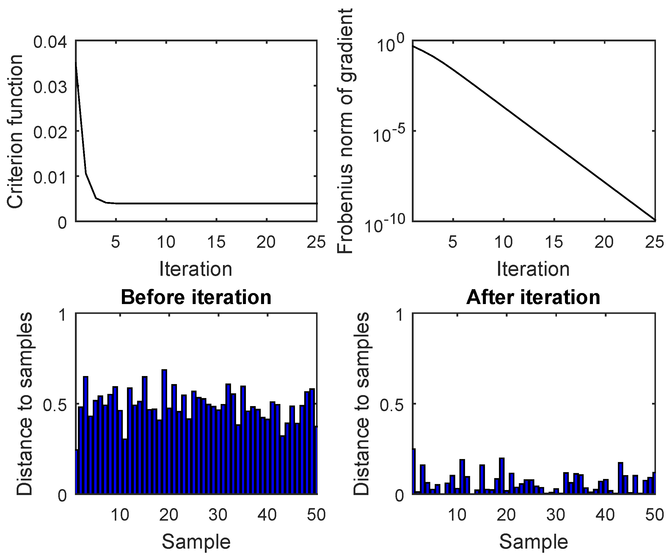
4.1. Gradient-Based Minimization of a Criterion Function Induced by the Frobenius Norm

The computation of the mean matrix from a dataset of matrices belonging to the pseudo-orthogonal group $O(1,1)$ is tackled as a first test. Further numerical tests focus on the computation of the empirical mean of a set of pseudo-orthogonal matrices in $O(p,q)$ with $p>1$ and $q>1$. All tests in the present section refer to Algorithm 1.

Numerical experiment A: Mean matrix computation on the pseudo-orthogonal group $O(1,1)$. From Lemma 4, we know that every element of the group $O(1,1)$ can be written in one of four canonical forms: here the first form is studied. This choice was motivated by the observation that the elements of the group $O(1,1)$ can be rendered graphically on a 2-dimensional drawing. Figure 1 shows the location of $N=50$ samples $X_k$ (circles) generated randomly around a randomly-selected center of mass (cross), the trajectory of the function minimization algorithm over $O(1,1)$ (solid-dotted line), and the location of the final point computed by the algorithm (diamond). To emphasize the behavior of the function minimization method in Equation (7), in the present experiment, a constant step-size schedule $t_{(\ell )}=\frac{1}{2}$ is selected and no stopping criterion is made use of. Figure 1 confirms that the numerical function minimization algorithm is convergent toward the center of mass. (Because of finite sample size, the empirical center of mass differs from the actual one.) Figure 2 shows the values of the criterion function $\frac{1}{2N}{\sum }_k{D}_{\mathrm{F}}^2(X,X_k)$ and of the Frobenius norm of its pseudo-Riemannian gradient during iteration, and the distances $D_{\mathrm{F}}(X,X_k)$ before iteration (with initial point chosen as $X_{(0)}=I_2$) and after iteration. In particular, all the distances from the samples $X_k$ and the matrix X decreased substantially.

Numerical experiment B: Mean matrix computation on the pseudo-orthogonal group $O(p,q)$ with $p,q>1$.Figure 3 illustrates a result obtained with the iterative algorithm in Equation (7) when $p=5,q=5$ and $N=50$. Figure 3 shows the values of the criterion function $\frac{1}{2N}{\sum }_k{D}_{\mathrm{F}}^2(X,X_k)$ and of the Frobenius norm of its pseudo-Riemannian gradient during iteration. Such numerical results were obtained by the adaptive step-size schedule explained in Section 2.2, the stopping condition in Equation (12) with precision $ϵ={10}^{-6}$ and an initial point chosen as $X_{(0)}=I_{10}$. Figure 3 also displays the distances $D_{\mathrm{F}}(X,X_k)$ before iteration (with initial point chosen as $X_{(0)}=I_{10}$) and after iteration. Figure 4 shows the value of the index $\parallel X_{(\ell )}^{\top }{R}_{p,q}{X}_{(\ell )}-R_{p,q}{\parallel }_F$ during iteration as well as the value of the step-size schedule. In Figure 4, the values of the coefficients ${\tilde{f}}_1$ and ${\tilde{f}}_2$ during iteration are displayed as well.

Figure 5 and Figure 6 illustrate the numerical results obtained by means of the iterative algorithm in Equation (7) for $p=10,q=5$ and $N=50$. As may be readily observed, with the growth of the dimension of the underlying manifold, the minimization problems related to the search for a mean matrix becomes increasingly harder to solve. Compared to the results shown in Figure 3 and Figure 4, the minimization algorithm takes a larger number of iterations to achieve comparable precision levels.

Figure 7 shows the result of an empirical statistical analysis about mean-matrix computation over the pseudo-orthogonal group $O(3,1)$ on 500 independent trials. In each trial, the algorithm starts from a randomly generated initial point. In particular, Figure 7 displays the distribution of the number of iterations that the numerical minimization algorithm takes to achieve the desired precision level $ϵ={10}^{-6}$ on each trial. The convergence speed varies with the initial point while the algorithm converges in every trial to the same value of the criterion function (namely, to about $0.0622$ in the current test). The largest number of trials converge in about 20–30 iterations.

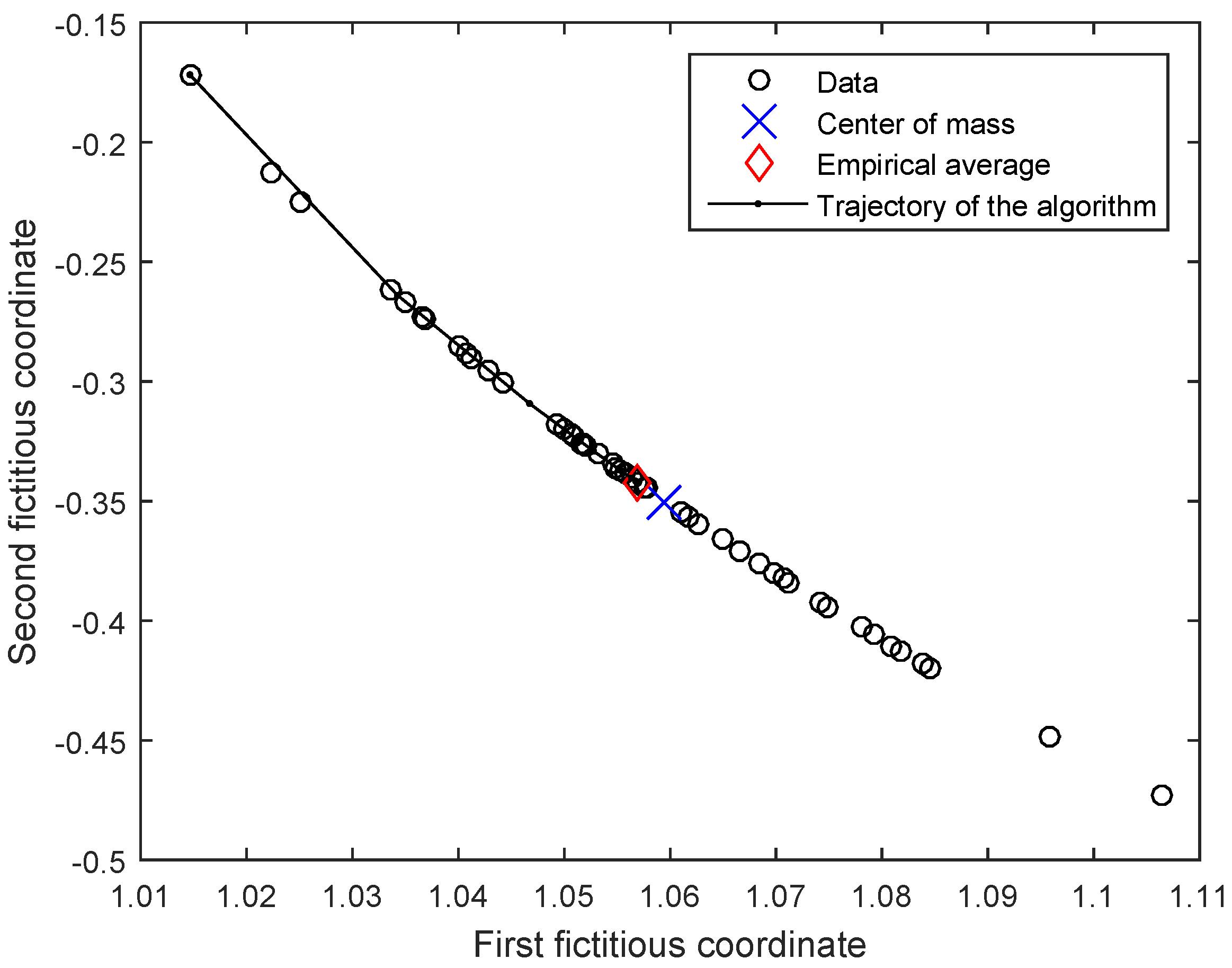
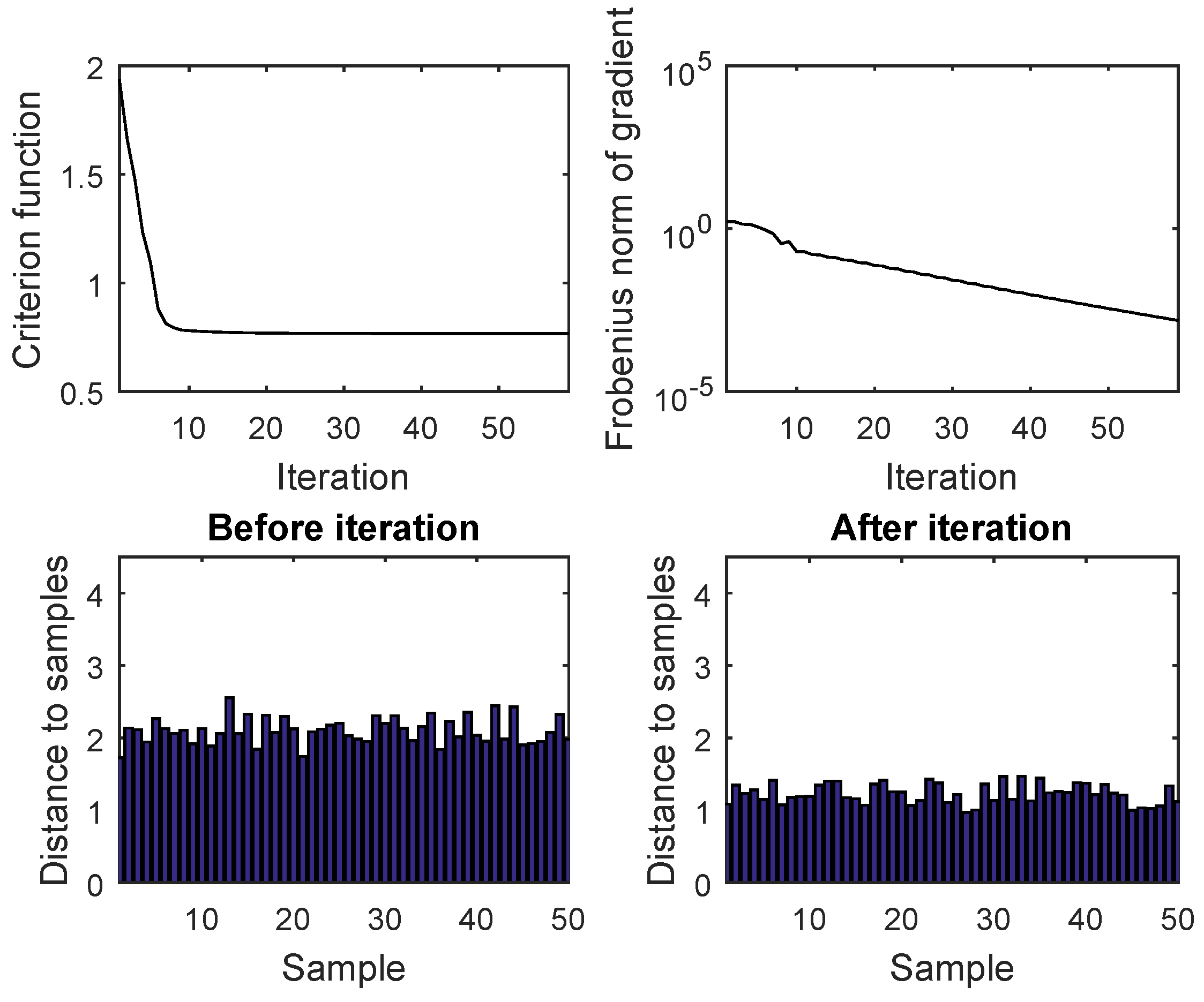
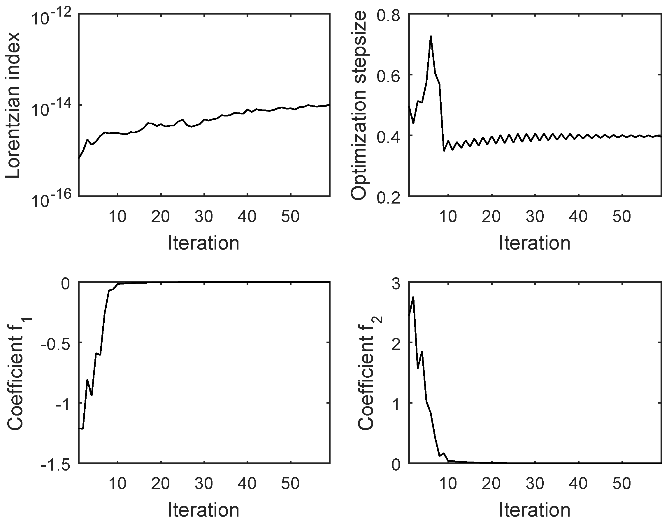
4.2. Gradient-Based Minimization of a Criterion Function Induced by the Geodesic Distance

In the following experiments, a constant step-size $\eta =\frac{1}{2}$ was chosen and, to evidence the numerical stability of the numerical minimization method, no stopping criterion was used. In this set of experiments, empirical means are sought for within the pseudo-orthogonal groups $O(1,1)$ and $O(5,5)$ by means of Algorithm 2.

Numerical experiment C: Mean matrix computation on the pseudo-orthogonal group $O(1,1)$.Figure 8 shows the results of optimization over the low-dimensional pseudo-orthogonal group $O(1,1)$ rendered on a 2-dimensional drawing. Figure 8 shows the location of 50 samples (or target matrices) $X_k$ (circles) generated randomly around a randomly-selected center of mass (cross), the location of the final point of the iteration, namely, the inferred empirical mean (diamond) and the trajectory of the function minimization algorithm over $O(1,1)$ (solid-dotted line). Figure 9 shows that the algorithm is convergent toward the center of mass. (Again, because of finite sample size, the empirical mean differs from the actual center of mass.) Figure 9 shows the values of the criterion function $\frac{1}{2N}{\sum }_k{D}_{\mathrm{g}}^2(X,X_k)$, the pseudo-norm of its pseudo-Riemannian gradient during iteration and the distances $D_{\mathrm{g}}(X,X_k)$ before iteration (with initial point chosen as $X_{(0)}=I_2$) and after iteration.

The numerical function-minimization algorithm converges steadily and quickly to the minimum value of the criterion function and keeps in the vicinity of the empirical mean after convergence.

Numerical experiment D: Mean matrix computation on the pseudo-orthogonal group $O(p,q)$ with $p,q>1$.Figure 10 shows a result obtained with the iterative algorithm (7) for $p=q=5$ and $N=50$. Figure 10 shows the values of the criterion function $\frac{1}{2N}{\sum }_k{D}_{\mathrm{g}}^2(X,X_k)$ and the pseudo-norm of its pseudo-Riemannian gradient during iteration, and the distances $D_{\mathrm{g}}(X,X_k)$ before iteration (with initial point chosen as $X_{(0)}=I_{10}$) and after iteration. The results in Figure 10 confirm that the numerical function minimization algorithm converges steadily toward the minimal distance configuration. In fact, the distances from the found empirical mean are much smaller than the distances from the initial point.

5. Conclusions

The present article investigated the computation of the empirical mean from a collection of pseudo-orthogonal matrices.

The pseudo-orthogonal group is regarded as a pseudo-Riemannian manifold and a metric is chosen that affords the computation of geodesic arcs in closed form as well as the pseudo-Riemannian gradient of a smooth function. Within such geometric setting, we consider a minimal-distance problem based on the Frobenius norm and on an induced geodesic distance. The related function minimization problem can be solved by a pseudo-Riemannian-gradient-based algorithm. Unlike the geodesic-based Riemannian gradient-steepest-descent function minimization method (see [11]), which converges under appropriate conditions, the geodesic-based stepping method (7) is not necessarily convergent, in general, due to the presence of the tangent-space component $T_x^{0}M$. However, the function minimization method (7), endowed with the step-size selection method (11), is shown numerically to enjoy favorable convergence properties in all numerical tests.

In this article, we present numerical tests based on two criterion functions. To illustrate the numerical features of the proposed function-minimization method, several indicators are defined and their values are evaluated on a number of case studies over the pseudo-orthogonal group in low as well as high dimension.

References

1. O’Neill, B. Semi-Riemannian Geometry. With Applications to Relativity. Pure and Applied Mathematics, 103; Academic Press, Inc.: New York, NY, USA, 1983. [Google Scholar]
2. Barachant, A.; Bonnet, S.; Congedo, M.; Jutten, C. Multi-class brain computer interface classification by Riemannian geometry. IEEE Trans. Bio-Med. Eng. 2012, 59, 920–928. [Google Scholar] [CrossRef] [PubMed]
3. Gariazzo, C.; Pelliccioni, A.; Bogliolo, M.P. Spatiotemporal analysis of urban mobility using aggregate mobile phone derived presence and demographic data: A case study in the city of Rome, Italy. Data 2019, 4, 8. [Google Scholar] [CrossRef]
4. Zavareh, M.; Maggioni, V. Application of rough set theory to water quality analysis: A case study. Data 2018, 3, 50. [Google Scholar] [CrossRef]
5. Sen, S.K. Classification on Manifolds. Ph.D. Thesis, Department of Statistics and Operations Research, University of North Carolina at Chapel Hill, Chapel Hill, NC, USA, 2008. [Google Scholar]
6. Bhattacharya, A.; Bhattacharya, R. Nonparametric Statistics on Manifolds with Applications to Shape Spaces. Pushing the Limits of Contemporary Statistics: Contributions in Honor of Jayanta K. Ghosh; Institute of Mathematical Statistics: Beachwood, OH, USA, 2008. [Google Scholar]
7. Freifeld, O. Statistics on Manifolds with Applications to Modeling Shape Deformations. Ph.D. Thesis, Division of Applied Mathematics, Brown University, Providence, RI, USA, 2014. [Google Scholar]
8. Celledoni, E.; Fiori, S. Descent methods for optimization on homogeneous manifolds. Math. Comput. Simulat. 2008, 79, 1298–1323. [Google Scholar] [CrossRef]
9. Fan, J.; Nie, P. Quadratic problems over the Stiefel manifold. Oper. Res. Lett. 2006, 34, 135–141. [Google Scholar] [CrossRef]
10. Gabay, D. Minimizing a differentiable function over a differentiable manifold. J. Optim. Theory Appl. 1982, 37, 177–219. [Google Scholar] [CrossRef]
11. Luenberger, D. The gradient projection method along geodesics. Manag. Sci. 1972, 18, 620–631. [Google Scholar] [CrossRef]
12. Wang, J.; Sun, H.; Li, D. A geodesic-based Riemannian gradient approach to averaging on the Lorentz group. Entropy 2017, 19, 698. [Google Scholar] [CrossRef]
13. Zhang, Z.Y.; Qiu, Y.Y.; Du, K.Q. Conditions for optimal solutions of unbalanced Procrustes problem on Stiefel manifold. J. Comput. Math. 2007, 25, 661–671. [Google Scholar]
14. Balande, U.; Shrimankar, D. SRIFA: Stochastic ranking with improved-firefly-algorithm for constrained optimization engineering design problems. Mathematics 2019, 7, 250. [Google Scholar] [CrossRef]
15. Hong, D.H.; Han, S. The general least square deviation OWA operator problem. Mathematics 2019, 7, 326. [Google Scholar] [CrossRef]
16. Mills, E.A.; Yu, B.; Zeng, K. Satisfying bank capital requirements: A robustness approach in a modified Roy safety-first framework. Mathematics 2019, 7, 593. [Google Scholar] [CrossRef]
17. Guo, D.; Li, B.; Zhao, W. Physical layer security and optimal multi-time-slot power allocation of SWIPT system powered by hybrid energy. Information 2017, 8, 100. [Google Scholar] [CrossRef]
18. Omara, I.; Zhang, H.; Wang, F.; Hagag, A.; Li, X.; Zuo, W. Metric learning with dynamically generated pairwise constraints for ear recognition. Information 2018, 9, 215. [Google Scholar] [CrossRef]
19. Duan, X.M.; Sun, H.F.; Peng, L.Y. Riemannian means on special Euclidean group and unipotent matrices group. Sci. World J. 2013, 2013, 292787. [Google Scholar] [CrossRef] [PubMed]
20. Moakher, M. A differential geometric approach to the geometric mean of symmetric positive-definite matrices. SIAM J. Matrix Anal. A 2005, 26, 735–747. [Google Scholar] [CrossRef]
21. Kaneko, T.; Fiori, S.; Tanaka, T. Empirical arithmetic averaging over the compact Stiefel manifold. IEEE Trans. Signal Proces. 2013, 61, 883–894. [Google Scholar] [CrossRef]
22. Fiori, S.; Kaneko, T.; Tanaka, T. Tangent-bundle maps on the Grassmann manifold: Application to empirical arithmetic averaging. IEEE Trans. Signal Proces. 2015, 63, 155–168. [Google Scholar] [CrossRef]
23. Fiori, S. Solving minimal-distance problems over the manifold of real symplectic matrices. SIAM J. Matrix Anal. A 2011, 32, 938–968. [Google Scholar] [CrossRef]
24. Başkal, S.; Georgieva, E.; Kim, Y.S.; Noz, M.E. Lorentz group in classical ray optics. J. Opt. B Quantum Semiclass. Opt. 2004, 6, S455–S472. [Google Scholar]
25. Podleś, P.; Woronowicz, S.L. Quantum deformation of Lorentz group. Commun. Math. Phys. 1990, 130, 381–431. [Google Scholar] [CrossRef]
26. Kawaguchi, H. Evaluation of the Lorentz group Lie algebra map using the Baker-Cambell-Hausdorff formula. IEEE Trans. Magn. 1999, 35, 1490–1493. [Google Scholar] [CrossRef]
27. Jost, J. Riemannian Geometry and Geometric Analysis; Springer: Berlin/Heidelberg, Germany, 2011. [Google Scholar]
28. Armijo, L. Minimization of functions having Lipschitz continuous first partial derivatives. Pac. J. Math. 1966, 16, 1–3. [Google Scholar] [CrossRef] [Green Version]
29. Baker, A. Matrix Groups: An Introduction to Lie Group Theory; Springer: Berlin, Germany, 2002. [Google Scholar]
30. Khvedelidze, A.; Mladenov, D. Generalized Calogero-Moser-Sutherland models from geodesic motion on GL+(n, R) group manifold. Phys. Lett. A 2002, 299, 522–530. [Google Scholar] [CrossRef]
31. Andrica, D.; Rohan, R.-A. A new way to derive the Rodrigues formula for the Lorentz group. Carpathian J. Math. 2014, 30, 23–29. [Google Scholar]
32. Wu, R.; Chakrabarti, R.; Rabitz, H. Critical landscape topology for optimization on the symplectic group. J. Optim. Theory Appl. 2010, 145, 387–406. [Google Scholar] [CrossRef]
Figure 1. Numerical test of function minimization applied to the criterion function in Equation (28) over the pseudo-orthogonal group O ( 1 , 1 ) : Data set and result of mean-matrix computation. (To obtain an easy-to-read graph, we chose to represent a pseudo-orthogonal matrix X O ( 1 , 1 ) , which is a 2 × 2 matrix, by two fictitious coordinates, namely the entry X ( 1 , 1 ) as first coordinate and the entry X ( 1 , 2 ) as second coordinate.)
Mathematics 07 00940 g001
Figure 2. Mean-matrix computation over the pseudo-orthogonal group O ( 1 , 1 ) : Values of the criterion function in Equation (28) during iteration, Frobenius norm of its pseudo-Riemannian gradient, distances D F ( X , X k ) before iteration ( X = X ( 0 ) ) and after iteration ( X = μ ) .
Mathematics 07 00940 g002
Figure 3. Mean-matrix computation over the pseudo-orthogonal group O ( 5 , 5 ) : Values of the criterion function in Equation (28) during iteration, Frobenius norm of its pseudo-Riemannian gradient, distances D F ( X , X k ) before iteration ( X = X ( 0 ) ) and after iteration ( X = μ ) .
Mathematics 07 00940 g003
Figure 4. Minimization of the criterion function in Equation (28) over the pseudo-orthogonal group O ( 5 , 5 ) : Values of the index X ( ) R p , q X ( ) R p , q F and of the coefficients t ^ ( ) , f ˜ 1 ( ) and f ˜ 2 ( ) during iteration.
Mathematics 07 00940 g004
Figure 5. Mean-matrix computation over over the pseudo-orthogonal group O ( 10 , 5 ) : Values of the criterion function in Equation (28) during iteration, Frobenius norm of its pseudo-Riemannian gradient, distances D F ( X , X k ) before iteration ( X = X ( 0 ) ) and after iteration ( X = μ ) .
Mathematics 07 00940 g005
Figure 6. Minimization of the criterion function in Equation (28) over the pseudo-orthogonal group O ( 10 , 5 ) : Values of the index X ( ) R p , q X ( ) R p , q F and of the coefficients t ^ ( ) , f ˜ 1 ( ) and f ˜ 2 ( ) during iteration.
Mathematics 07 00940 g006
Figure 7. Minimization of the criterion function in Equation (28) over the pseudo-orthogonal group O ( 3 , 1 ) : Distribution of the number of iterations to converge on each trial on a total of 500 independent trials.
Mathematics 07 00940 g007
Figure 8. Minimization of the criterion function in Equation (38) over the pseudo-orthogonal group O ( 1 , 1 ) : Data set and result of mean-matrix computation.
Mathematics 07 00940 g008
Figure 9. Mean-matrix computation over over the pseudo-orthogonal group O ( 1 , 1 ) : Values of the criterion function in Equation (38) during iteration, of the pseudo-norm of its pseudo-Riemannian gradient, of the distances D g ( X , X k ) before iteration ( X = X ( 0 ) ) and after iteration ( X = μ ) .
Mathematics 07 00940 g009
Figure 10. Mean-matrix computation over the pseudo-orthogonal group O ( 5 , 5 ) : Values of the criterion function in Equation (38) during iteration, of the pseudo-norm of its pseudo-Riemannian gradient, of the distances D g ( X , X k ) before iteration ( X = X ( 0 ) ) and after iteration ( X = μ ) .
Mathematics 07 00940 g010