Abstract
A natural extension of maximum flow problems is called the generalized maximum flow problem taking into account the gain and loss factors for arcs. This paper investigates an inverse problem corresponding to this problem. It is to increase arc capacities as less cost as possible in a way that a prescribed flow becomes a maximum flow with respect to the modified capacities. The problem is referred to as the generalized maximum flow problem (IGMF). At first, we present a fast method that determines whether the problem is feasible or not. Then, we develop an algorithm to solve the problem under the max-type distances in time. Furthermore, we prove that the problem is strongly NP-hard under sum-type distances and propose a heuristic algorithm to find a near-optimum solution to these NP-hard problems. The computational experiments show the accuracy and the efficiency of the algorithm.
1. Introduction
In a capacitated network, the conventional maximum flow problem is to look for maximum flow which can be sent from a source to a sink under arc capacity constraints. The flow is conserved on arcs and the flow that enters any node (except the source and the sink) equals the flow leaving it.
In the generalized network flow problem, we have a gain factor for every arc. This gain factor represents the amount of flow that arrives at node j if we would send one unit of flow from the node i along arc . More specifically, if we send units from i to j, then units arrive at node j. These gains or losses can refer to evaporation, energy dissipation, breeding, theft, interest rates, blending, or currency exchange. The generalized maximum flow problem can be formulated as a linear programming problem [1]. The augmenting path algorithm and its variants are first algorithms to be proposed for solving the problem [2,3]. A close relationship between this problem and the minimum cost flow problem [4] is stated in Truemper [5]. This fact clarifies that many algorithms of generalized maximum flow problems are similar to those of minimum cost flow problems. Tardos and Wayne [6] developed the first efficient primal algorithm for solving the problem and extend the algorithm for generalized minimum cost flow problem. However, a strongly polynomial-time algorithm that is not based on general linear programming techniques is given for the generalized flow maximization problem in [7], which using a new variant of the scaling technique. Then, another strongly polynomial-time algorithm is developed in [8]. It is faster and simpler than the preceding ones. It works almost exclusively with integral flows, in contrast to all previous algorithms.
For any optimization problem, one can define a corresponding inverse problem. It is how to modify some parameters, such as costs or capacities, in a way that a prescribed solution of the optimization problem becomes optimal with respect to the new parameters. The objective function of inverse problems is to minimize the distance between the initial and new parameters. The changes can be calculated by Hamming distances or norms. Due to wide range of applications, many researchers have focused on inverse optimization problems in recent years [9,10,11,12,13,14,15,16,17,18,19]. Let us review some papers concerning the inverse maximum flow problem. Yang et al. [20] presented strongly polynomial-time algorithms to solve the inverse maximum flow problem under norm. In [21,22,23], efficient algorithms are proposed to solve the inverse maximum flow problem with lower and upper bounds, considering the norms and . Inverse maximum flow problems under the bottleneck-type () and sum-type () Hamming distances are also investigated in [24]. Strongly polynomial algorithms are proposed for these problems. The general result is that the inverse maximum flow problem under and can be solved in strongly polynomial time.
The reverse problems are another kind of inverse optimization problem. In the reverse maximum flow problem, the goal is to change arc capacities minimally so that the maximum flow value becomes at least a prescribed value . The problem is studied in [25] under weighted norm. The authors presented an efficient algorithm based on the discrete-type Newton method to solve the problem.
In this paper, we study the inverse generalized maximum flow problem (denoted IGMF). First we start with an apriori test with a good complexity of which decides whether the problem is feasible or not. Then, we develop an efficient algorithm to solve the problem under the max-type distances and . By a reduction of the vertex cover problem, we prove that the problem under the sum-type distances and is strongly NP-hard. This result is interesting because the (ordinary) inverse maximum flow problems under the sum-type distances are solved in strongly polynomial time [23,24]. Finally, we present a heuristic algorithm to find pseudo-optimal solutions to the problem.
We recall the definitions of weighted and weighted norms for the n-dimensional vector x:
where is the per unit cost attached to the i-th component. A natural use of the norms is that they can be applied to measure the distance between two vectors x and y as , . For this reason, the word “distance” is also used instead of “norm” for these functions.
The definitions of the sum-type and bottleneck-type Hamming distances for two n-dimensional vectors x and y are given as follows:
where is the cost of modification associated with the i-th component. The function H measures the Hamming distance between the real values and which is defined as follows:
The rest of the paper is organized as follows: In Section 2, we focus on the generalized maximum flow problem and state its optimality conditions. In Section 3, we introduce the inverse generalized maximum flow problem and we study its feasibility. In Section 4, we present our proposed algorithm to solve the IGMF for the max-type distances. In Section 5, study IGMF under the sum-type distances and . We prove that these problems are strongly NP-hard. In Section 6, we present a heuristic algorithm for these problems. In Section 7, we perform several computational experiments to consider the accuracy and efficiency of the heuristic algorithm. Finally, some concluding remarks are given in Section 8.
2. The Generalized Maximum Flow
We denote by a generalized network, where N is a set of n-nodes, A is a set of m directed arcs, s and t are special nodes called the source and the sink, respectively. is the capacity function and is the gain function.
The gain of a path P is denoted by . In the same manner, we define the gain of a cycle. A flow-generating cycle is a cycle C whose gain is more than one, i.e., .
We assume that G has no parallel arcs. Without loss of generality we also assume that the network is symmetric, which means that for each arc there is an arc possibly with zero capacity. The gain function is antisymmetric, i.e., .
A function that satisfies the capacity constraints for every and the antisymmetry constraints for every is called a generalized pseudoflow. The residual excess of a node i, except s, is (the negative of the flow that leaves node i). If is positive (negative), we say that f has residual excess (deficit) at node i. A pseudoflow f is a flow if it has no residual deficits and residual excesses, except in s and t. For a flow f, we denote its value to be the residual excess at the sink.
For a generalized flow f in we can define the residual capacity function
The residual network is in which . The generalized maximum flow problems in the initial network and the residual network are equivalent together. A path in the residual network from an excess node to the sink is called an augmenting path. A flow-generating cycle together with one path from some nodes of this cycle to the sink is referred to as a generalized augmenting path (GAP). One can increase the flow into the sink by sending flow along GAPs and augmenting paths. We shall take an example now.
Example 1.
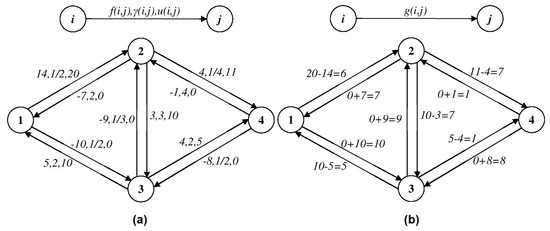
In Figure 1a we have a network flow in a generalized network with the source node 1 and the sink node 4. We suppose that , . It is easy to see that f satisfies the capacity constraints and the antisymmetry constraints, so, it is a pseudoflow. Let us calculate the residual excesses: , and . It is clear now that the pseudoflow f have not any residual deficits (excesses) and, so, it is a flow in the generalized network from Figure 1a. Obviously, . The corresponding residual network is presented in Figure 1b. In this network, we have a flow-generating cycle: whose gain factor is equal to .
Figure 1.
Calculating the residual network for generalized network flows.
The following theorem gives us the optimality conditions for the problem (see [3]):
Theorem 1.
A flow f is optimal in a generalized network G if and only if there is no augmenting path and no GAP in .
Assume that each arc is associated with a cost of . To find a GAP in the residual network , we first apply the BFS algorithm to identify the part of the network with nodes which have paths to t. Then, we look after a negative cost cycle C with respect to the arc costs in this part of the network. Notice since
it is guaranteed that is a GAP where P is a path found by the BFS algorithm from some nodes of C to t. The complexity of this process is because the complexity of the BFS algorithm is and we can use the shortest path algorithm due to Bellman-Ford to find a negative cost in [1]. Since the computation of logarithms is time-consuming and inexact in computers, it is not customary to calculate logarithms. However, one can work directly with the gain factors (multiplying gain factors of arcs instead of adding costs of arcs). This yields a modified version of Bellman-Ford algorithm which finds a flow-generating cycle in time.
Using the fact that the generalized maximum flow problem is a linear programming, the optimality conditions of linear programming problems can be also used to check the optimality of a flow. For this purpose, suppose that a real number is associated with each node i. Indeed, , called the potential of node i, is the dual variable corresponding to the ith balanced constraint. By noting the dual of the problem, it is easy to see that and . The potential difference of an arc is defined as . The following theorem gives the optimality conditions of a feasible flow to the generalized maximum flow problem.
Theorem 2.
A flow f is optimal to the generalized maximum flow problem if and only if there are node potentials π such that
- for every ;
- for every ;
- for every .
Proof.
See Theorem 15.5 in [1]. □
3. Inverse Generalized Maximum Flow Problem
Let be a generalized network. Let f be a feasible flow in the network G. It means that f must satisfy the capacity restrictions, the antisymmetry constraints and it must have no residual deficits and residual excesses (except in s and t).
The inverse generalized maximum flow problem is to change the capacity vector u so that the given feasible flow f becomes a maximum flow in G and the distance between the initial vector of capacities u and the modified vector of capacities, denoted by , is minimized:
where and are the given non-negative numbers to determine bounds on the modifications and , for each arc (see notations of [19]). These values show how much the capacities of the arcs can vary.
It is easy to see that to transform the flow f into a maximum flow in the network , it is useless to increase the capacities of the arcs. Therefore, the conditions , for each arc have no effect and, instead of (8), we consider the following mathematical model:
When solving IGMF, if the capacity is changed on arc , then it is decreased exactly with the amount of units. If not so, the flow is not stopped from being increased on an augmenting path from s to t or in a GAP that contains the arc and the modification of the capacity of is useless. This implies that when solving IGMF, it is no need to change the capacities of the arcs from the following set:
The set is a subset of . Observe that it contains all arcs of G with , because .
The above argument together with Theorem 2 suggest a zero-one formulation for IGMF:
in which the zero-one variable is defined as if and only if . A simple statement of the formulation (11) is that some arcs belonging to have to be transported to U by setting . Consequently, their corresponding constraint, namely , is relaxed to (see the constraints (11c) and (11e)). Furthermore, setting , , removes from the network, so the constraint is also relaxed (see the constraint (11g)). The formulation (11) is a zero-one linear programming under all the norms and the Hamming distances and . So, one can use the zero-one programming technique to solve the problem.
To verify the feasibility of IGMF we construct the network in which is defined in (10).
Theorem 3.
IGMF is feasible in the generalized network G for a given flow f, if and only if there is no directed path in from the node s to the node t and there is no GAP in .
Proof.
If IGMF is a feasible problem, then it means that there is a vector with , and for which the flow f is a maximum flow in the network . Since , if there exists a directed s-t path in , it corresponds to a directed path in , which leads to an augmentation to the flow f in G (contradiction). If there is a GAP in , then it is a GAP in (contradiction).
Now, for the inverse implication we construct the following capacity vector:
It is easy to see that , . In the residual network corresponding to with respect to the flow f, we have , for every . Hence, . Since there is no directed path from s to t and no GAP in , it follows that there is no directed path from s to t and no GAP in . So f is a maximum flow in . Consequently, is a feasible solution for IGMF. □
The feasibility of IGMF can be determined in time complexity because it uses a graph search algorithm in which can be done in time and the adapted Bellman-Ford algorithm in which is run in time [1].
4. Algorithms for Solving IGMF under Max-Type Distances
Now we study IGMF under max-type distances (denoted IGMFM). This means that in the problem (9) is defined as follows:
where . It is easy to see that the bottleneck-type Hamming distance defined in (4) is a particular case of (12) because
where is the cost of modification of the capacity on the arc .
IGMF under weighted norm (denoted IGMF) can be also treated as a particular case of IGMFM. For IGMF, we define
where is per unit cost of modification of the capacity on the arc .
Suppose that IGMFM is feasible. The algorithm for IGMFM begins with a set . So, the elimination of all arcs from H transforms the flow f into a maximum flow in the resulting network. So, we have to find a subset J of H so that if the arcs of J are eliminated then f becomes a maximum flow in the resulting network and the modified capacity vector is optimum for IGMFM. To do this, arcs of H are sorted in nondecreasing order by their value . Arcs are eliminated sequentially from H (from arc with the lowest value to the highest) until the arcs of form a graph in which there is no directed path from s to t and there are no GAPs. The arcs that leave the set H are the arcs where the capacities are modified to the value . Based on Theorem 1, the flow f is a maximum flow in the resulting network. Let us write the algorithm, formally.
Theorem 4 (the correctness).
The vector found by Algorithm 1 is the optimal solution of IGMFM.
Proof.
Assume that is an optimal solution of IGMF with the optimal value . By contradiction, we suppose that
We construct the capacity vector as follows:
It is easy to see that is also optimal solution for IGMF. On the other hand, due to (13), is constructed and tested before constructing . This test failed because the algorithm does not terminate in that iteration. Therefore, is not optimal solution for IGMF which is a contradiction. □
Theorem 5 (the complexity).
The algorithm IGMFM runs in time.
Proof.
The feasibility initial test is performed in time. The vector H can be sorted in time, using an efficient sorting algorithm, for instance QuickSort [26]. The set H contains at most m arcs. If all the arcs of H are eliminated, then f is a maximum flow in the resulting . Therefore, after at most m iterations of the loop f becomes maximum and the algorithm ends. It takes time to test if there is a directed path from s to t in and time to test if there is a GAP in . Consequently, testing if f is a maximum flow takes time. Therefore, the total time of the algorithm is . □
| Algorithm 1: Algorithm to solve IGMFM |
| Input: The generalized network and flow f. |
| Output: is the optimal solution of the IGMFM problem. |
| Construct the residual network . |
| Set . |
| Construct the network . |
| If The problem is not feasible (there is an s-t directed path or a GAP in ) |
| Stop. |
| End If |
| Set and . |
| Sort arcs of H in nondecreasing order with respect to . |
| Whilef is not a maximum flow in |
| Let the first arc from H. |
| . |
| . |
| End While |
We can improve the running time of the IGMFM algorithm by using a “Divide and Conquer” approach. We test the optimality of f after we removed the arcs from the first half of H. We have two situations:
- Case 1. If f is a maximum flow in , then we remove only the first quarter of what was initially in H.
- Case 2. If f is not a maximum flow in , then we remove also the first half of what remained in H.
The “Divide and Conquer” technique continues until no division can be done any more. The “Divide and Conquer” version of Algorithm 1 is as Algorithm 2.
Since the algorithm deals with the same idea as Algorithm 1, its correctness is obvious. Then, we discuss only about its complexity.
Theorem 6.
The time complexity of the improved IGMFM algorithm is .
Proof.
The feasibility test can be performed in time. The vector H can be sorted in . Instead of iterations, the “Divide and Conquer” version has iterations. Therefore, the time complexity of "Divide and Conquer" algorithm is , since each iteration takes at most time. □
| Algorithm 2: The “Divide and Conquer” version of Algorithm 1 |
| Input: The generalized network and flow f. |
| Output: is the optimal solution of the IGMFM problem. |
| Construct the residual network . |
| Set . |
| Construct the network . |
| If The problem is not feasible (there is an s-t directed path or a GAP in ) |
| Stop. |
| End If |
| Set and . |
| Sort the arcs of H in nondecreasing order with respect to : let is the sorted list. |
| Set and . |
| While |
| Set , . |
| . |
| For do |
| Set . |
| End For |
| If f is a maximum flow in |
| Set . |
| Else |
| Set , and . |
| End If |
| End While |
5. IGMF under Sum-Type Distance
In this section, we consider IGMF under the sum-type distances and . We prove that IGMF under these distances is strongly NP-hard. The proof is based on a reduction from the node cover problem. Let us first recall this problem.
The node cover problem:
- Instance, an undirected network and a given number k.
- Question, is there a set so that and S is a node cover of , i.e., either or for every ?
Theorem 7.
The inverse generalized maximum flow problem under the norm is strongly NP-hard.
Proof.
Suppose that an instance of the node cover problem defined on an undirected graph is given, where is the node set and is the arc set. We introduce a bipartite directed network as follows:
- The network contains two nodes i and , for each . Additionally, we add three nodes to the network. Using the notation , we have .
- For each undirected arc , we add two directed arcs and to G. We also add for and for . We call all these arcs the natural arcs. Then the set of natural arcs is:We associate with each , one arc . Such arcs are referred to as the artificial arcs, denoted by . Thus, . Please note that the underlying undirected graph of G is bipartite.
- The gain of each natural arc is equal to 1 while the gain of each artificial arcs is 2.
- The capacity of each natural arc is equal to . The capacity of each artificial arc is 1.
- for every .
□
Figure 2 shows an example of how to construct G from . Let be the initial flow. Since the data are polynomially bounded with respect to the problem size, i.e., the similarity assumption is satisfied, we prove the following claim to establish the desired result.
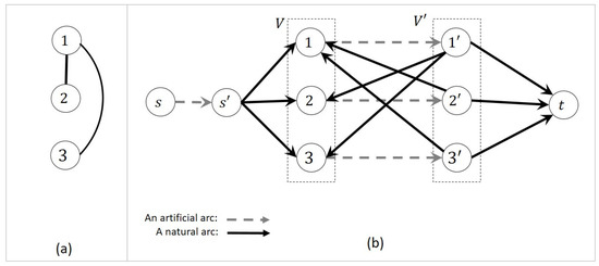
Figure 2.
To construct the directed network G from the undirect graph .
Claim 1.
The node cover problem in is a yes instance if and only if there is a feasible solution to the inverse generalized maximum flow problem in G with the objective value at most equal to .
Proof of Claim 1.
Suppose that S is a solution to a given yes instance of the node cover problem. We introduce the solution as follows:
It is easy to see that the objective value of is less than or equal to . Thus, it is sufficient to prove that the residual network with respect to the flow and the capacity vector contains no -path and no GAP. Because is not in the residual network, we imply that any st-path does not exists in the residual network. Since all gain factors are greater than or equal to 1 and any cycle contains at least an arc with , it follows that any cycle in the residual network is a part of a GAP. Then, we must prove that the residual network contains no cycle. Any cycle has at least two arcs from to and at least two arcs from to . Then it contains a path . Due to this and that , we imply that or . Equivalently, or . Therefore, the residual network does not contain at least one of two the arcs and . Then, any cycle cannot exist in the residual network.
Now suppose that is a feasible solution to the inverse generalized maximum flow problem with the objective value . The assumption guarantees that for each arc which has infinity capacity. Hence, only the capacity of artificial arcs can be modified. Consider . We prove that S is a cover of with . Any st-path in G is . Since the residual network contains no st-path, two cases may occur:
- is not in the residual network.
- Each arc , , is not in the residual network.
The first case imposes a cost of 1 on the objective while the second imposes a cost of . Then, due to the optimality of , the first case occurred, namely . On the other hand, we know that the residual network contains no cycle (GAP). Then, or for each cycle . This implies that or for each . Then, S is a cover of with . This completes the proof. □
A completely similar proof proves that IGMF under is NP-hard. In the proof. it is sufficient to define the capacity of all arcs equal to 1 and the weight vector w as
Thus, we have the following result.
Theorem 8.
The inverse generalized maximum flow problem under the sum-type Hamming distance is strongly NP-hard.
6. A Heuristic Algorithm
In this section, we present a heuristic algorithm to obtain pseudo-optimal solutions of IGMF under the sum-type distances.
To remove a GAP C, we must remove an arc by setting . We use the five following observations to design our algorithm.
- An arc cannot be removed from the residual network because setting violates the bound constraint.
- A necessary condition for removing arc is that it belongs to at least one GAP.
- An arc belonging to several GAPs has a high priority to be removed because several GAPs are annihilated whenever we remove such an arc.
- Removing of an arc imposes the cost of ( ) to the objective function under ().
- If an arc is on a GAP C so that the other arcs of C belong to , then the arc has the greatest priority to be removed because we can eliminate C only by removing .
We now introduce a preference index , , to determine which one of arcs has high priority to be removed. Based on Observations 3 and 4, an arc is eligible to be removed if
- it is on a greater number of GAPs, and
- it imposes a smaller value of the cost on the objective function.
So, we define
for every in which is a value to underestimate how many GAPs pass through . To compute ’s, we use a successive negative-cycle subroutine. The subroutine initializes for each . In each iteration, it detects a GAP by using the Reverse Bellman-Ford (RBF) algorithm which has the same process of the standard Bellman-Ford algorithm with this difference which it starts from t and traverses arcs in the opposite direction. The RBF algorithm detects a negative-cycle with respect to the arc lengths in residual network. The output of the RBF algorithm is a negative-cycle together with a path P from some nodes of to t. Since any negative cycle with respect to is also a generating flow cycle (see (7)), it follows that is a GAP. After detecting a GAP C by the RBF algorithm, the subroutine determines its capacity, i.e., . Then, it updates and for each and it removes arcs with . The process is repeated until any negative cycle is not detected by the RBF algorithm. It is notable that if a GAP C contains no arc of , then the problem is infeasible (see Theorem 3). To handle this situation, another output is defined for the subroutine which is a Boolean variable and takes the value of if the subroutine detects this situation. According to Observation 5, another specific situation may occur in which all arcs of the successive negative-cycle GAP belong to , except one arc . In this situation, the subroutine sets which is a very big number. Algorithm 3 states the process of the subroutine, formally. Notice that if , then there is not any GAP passing through (Observation 1). Therefore, the arc has the lowest priority to be removed.
The main algorithm in each iteration calls the subroutine for computing . Then, it calculates the priority index for each arc . Finally, it chooses one arc of A with the maximum priority index and remove it from the residual network by setting . This process is repeated until the residual network contains no GAP. Our proposed algorithm is given in Algorithm 4.
| Algorithm 3: The successive negative-cycle algorithm |
| Input: The network , the arc set . |
| Output: The priority degrees v as well as the Boolean variable which is if the algorithm detects the infeasibility. |
| Fordo |
| Set . |
| EndFor |
| Set . |
| While True |
| Apply the Reverse Bellman-Ford algorithm starting t to find a negative-cycle C with respect to the arc lengths . |
| If There is no negative cycle Break. |
| End If |
| Set . |
| Set . |
| For do |
| Set . |
| Set . |
| If |
| Remove from . |
| End If |
| If |
| Set . |
| Set . |
| End If |
| End For |
| If %See Theorem 3. |
| Set . |
| Break. |
| End If |
| If %See Observation 5. |
| Set %M is a very big integer |
| Break. % is the only arc that can cancel C |
| End If |
| End While |
Remark 1.
If we define the priority index as follows:
then Algorithm 4 is a heuristic algorithm to obtain a pseudo-optimal solution to the problem under .
Now, let us argument about the complexity of Algorithm 4. The RBF algorithm similar to the standard Bellman-Ford algorithm has a time complexity of [1]. Since Algorithms 3 and 4 remove at least one arc in each iteration, then they terminate in iterations. Hence, we have the following result.
Theorem 9.
Algorithm 4 runs in time.
| Algorithm 4: A heuristic algorithm to solve IGMF under |
| Input: The generalized network and flow f. |
| Output: The modified capacity vector . |
| Set . |
| Construct the residual network . |
| Set . |
| For each do |
| If |
| Add arc to . |
| End If |
| End For |
| While True |
| Apply Algorithm 3. Suppose that the output is . |
| If |
| Stop because the problem is infeasible. |
| End If |
| Set |
| For do |
| If and |
| Set . |
| If |
| Set and . |
| End If |
| End If |
| End For |
| If |
| Break. |
| Else |
| Set . |
| Remove from . |
| End If |
| End While |
7. Computational Experiments
In this section, we have conducted a computational study to observe the performance of Algorithm 4. To study its accuracy, we compared the results obtained by Algorithm 4 with the exact optimal solution which is computed by solving the model (11).
The following computational tools were used to develop Algorithm 4 and to solve model (11): Python 2.7.5, Matplotlib 1.3.1, Pulp 1.6.0, and NetworkX 1.8.1. All computational experiments were conducted on a 64-bit Windows 10 with Processor Intel(R) Core(TM) i CPU GHz and 4 GB of RAM.
In experiments, we have applied random binomial graphs introduced in [27]. These graphs are determined by two parameters n, the number of nodes, and which is the probability of existing any edge in the graph. In experiments, we have first generated an undirected graph and then have converted it into a directed one by directing any edge from i to j if . In all experiments, we have assumed that nodes and are respectively the source and the sink.
All data are generated randomly by using a uniform random distribution as follows:
Our experiments show to Algorithm 4 correctly detects the infeasibility of the problem. For this reason, we set for each to guarantee the feasibility of instances. To generate a feasible flow, we added a node and an arc with capacity . Then, we found a maximum flow f from to . The flow f saturates , then it is a feasible solution with the flow value . After computing f, we removed the dummy node as well as the arc from the network. The following computational results are the average of running Algorithm 4 on 100 different instances of a class.
We have tested Algorithm 4 on 12 classes of networks which differ from the number of nodes, varying from 5 to 60 (see Table 1). In the tables, is the optimal value and z is the objective value obtain by the algorithm. Since Algorithm 4 finds correctly the solution whenever , the results are reported in two cases: total results and results for problems whose optimal value is nonzero. In both the cases, we reported the values and . We also tested Algorithm 4 on 9 classes of networks which differ from the density, varying from to 1. The results are shown in Table 2.

Table 1.
Average performance statistics of Algorithm 4 for the graphs with .
Table 2.
Average performance statistics of Algorithm 4 for the graphs with .
In another experiment, we run the algorithm 1000 time for and . Then, we classify instances with respect to their optimal value. The results of this experiment are available in Table 3 and are depicted in Figure 3. Observe that the error is lesser when the optimal value is nearer to zero.
Table 3.
Average performance statistics of Algorithm 4 for and .
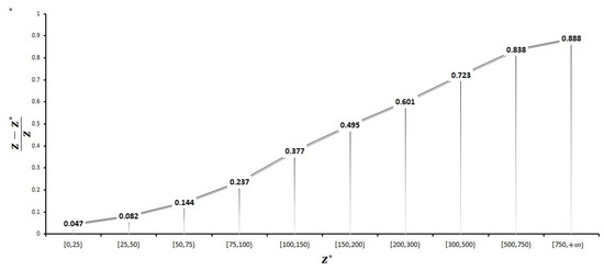
Figure 3.
Error chart: X-axis is the intervals containing the optimal value and Y-axis is .
8. Conclusions
In this paper, we have studied two classes of inverse problems: IGMF under max-type distances and under sum-type distances. We have provided a fast initial test of feasibility of IGMF. For the first class we presented polynomial algorithms to solve IGMF in running time and even in ) time. We proved that the second class of problems are NP-hard and we presented a heuristic algorithm to solve this kind of problems.
As future works, it will be meaningful that other types of inverse generalized maximum flow problem are investigated. Specifically, one may consider a type of the inverse problem for which gain factors are modified, instead of capacities. This problem can be used to simulate a wide range of real-world applications because gain factor modifications are performed by network restorations.
Author Contributions
All the authors contributed equally to this manuscript.
Funding
This research was funded by Transilvania University of Brasov.
Conflicts of Interest
The Authors declare no conflict of interest.
References
- Ahuja, R.K.; Magnanti, T.L.; Orlin, J.B. Network Flows: Theory, Algorithms, and Applications; Prentice Hall: Englewood Cliffs, NJ, USA, 1993. [Google Scholar]
- Jewell, W.S. Optimal flow through networks with gains. Oper. Res. 1962, 10, 476–499. [Google Scholar] [CrossRef]
- Onaga, K. Dynamic programming of optimum flows in lossy communication nets. IEEE Trans. Circuit Theory 1966, 13, 308–327. [Google Scholar] [CrossRef]
- Ciupala, L. A scaling out-of-kilter algorithm for minimum cost flow. Control Cybern. 2005, 34, 1169–1174. [Google Scholar]
- Truemper, K. On max flows with gains and pure min-cost flows. SIAM J. Appl. Math. 1977, 32, 450–456. [Google Scholar] [CrossRef]
- Tardos, E.; Wayne, K.D. Simple Generalized Maximum Flow Algorithms. Integer. Program. Comb. Optim. 1998, 1412, 310–324. [Google Scholar]
- Vegh, L.A. A strongly polynomial algorithm for generalized flow maximization. Math. Oper. Res. 2016, 42, 179–211. [Google Scholar] [CrossRef]
- Olver, N.; Vegh, L.A. A simpler and faster strongly polynomial algorithm for generalized flow maximization. In Proceedings of the 49th Annual ACM SIGACT Symposium on Theory of Computing, ACM 2017, Montreal, QC, Canada, 19–23 June 2017; pp. 100–111. [Google Scholar]
- Ahuja, R.K.; Orlin, J.B. Combinatorial Algorithms for Inverse Network Flow Problems. Networks 2002, 40, 181–187. [Google Scholar] [CrossRef]
- Ciurea, E.; Deaconu, A. Inverse Minimum Flow Problem. J. Appl. Math. Comput. 2007, 23, 193–203. [Google Scholar] [CrossRef]
- Demange, M.; Monnot, J. An introduction to inverse combinatorial problems. In Paradigms of Combinatorial Optimization (Problems and New approaches); Paschos, V.T., Ed.; Wiley: London, UK; Hoboken, NJ, USA, 2010. [Google Scholar]
- Heuberger, C. Inverse Combinatorial Optimization, A Survey on Problems, Methods, and Results. J. Comb. Optim. 2004, 8, 329–361. [Google Scholar] [CrossRef]
- Karimi, M.; Aman, M.; Dolati, A. Inverse Generalized Minimum Cost Flow Problem Under the Hamming Distances. J. Oper. Res. Soc. China 2019, 7, 355–364. [Google Scholar] [CrossRef]
- Liu, L.; Zhang, J.; Li, C. Inverse minimum flow problem under the weighted sum-type Hamming distance. Discrete Appl. Math. 2017, 229, 101–112. [Google Scholar] [CrossRef]
- Liu, L.; Yao, E. Capacity inverse minimum cost flow problems under the weighted Hamming distance. Optim. Lett. 2016, 10, 1257–1268. [Google Scholar] [CrossRef]
- Nourollahi, S.; Ghate, A. Inverse optimization in minimum cost flow problems on countably infinite networks. Networks 2019, 73, 292–305. [Google Scholar] [CrossRef]
- Tayyebi, J.; Aman, M. On inverse linear programming problems under the bottleneck-type weighted Hamming distance. Discrete Appl. Math. 2018, 240, 92–101. [Google Scholar] [CrossRef]
- Tayyebi, J.; Massoud, A.M. Efficient algorithms for the reverse shortest path problem on trees under the hamming distance. Yugoslav J. Oper. Res. 2016, 27, 46–60. [Google Scholar] [CrossRef]
- Zhang, J.; Cai, C. Inverse Problems of Minimum Cuts, ZOR-Math. Methods Oper. Res. 1998, 47, 51–58. [Google Scholar] [CrossRef]
- Yang, C.; Zhang, J.; Ma, Z. Inverse Maximum Flow and Minimum Cut Problems. Optimization 1997, 40, 147–170. [Google Scholar] [CrossRef]
- Ciupala, L.; Deaconu, A. Inverse maximum flow problem in planar networks. Bull. Transilv. Univ. Brasov Math. Inform. Phys. Ser. III 2019, 12, 113–122. [Google Scholar]
- Deaconu, A. The Inverse Maximum Flow Problem Considering L∞ Norm. RAIRO-Oper. Res. 2008, 42, 401–414. [Google Scholar] [CrossRef][Green Version]
- Deaconu, A. The inverse maximum flow problem with lower and upper bounds for the flow. Yugoslav J. Oper. Res. 2016, 18, 13–22. [Google Scholar] [CrossRef]
- Liu, L.; Zhang, J. Inverse Maximum Flow Problems under Weighted Hamming Distance. J. Combin. Optim. 2006, 12, 395–408. [Google Scholar] [CrossRef]
- Tayyebi, J.; Mohammadi, A.; Kazemi, S.M.R. Reverse maximum flow problem under the weighted Chebyshev distance. RAIRO-Oper. Res. 2018, 52, 1107–1121. [Google Scholar] [CrossRef]
- Hoare, C.A.R. Algorithm 64: Quicksort. Commun. ACM 1961, 4, 321. [Google Scholar] [CrossRef]
- Erdõs, P.; Rényi, A. On Random Graphs. I. Publ. Math. 1959, 6, 290–297. [Google Scholar]
© 2019 by the authors. Licensee MDPI, Basel, Switzerland. This article is an open access article distributed under the terms and conditions of the Creative Commons Attribution (CC BY) license (http://creativecommons.org/licenses/by/4.0/).