The Modified Beta Gompertz Distribution: Theory and Applications


 ,
, 
Abstract
:1. Introduction
2. The Modified Beta Gompertz Distribution
- When with ( is a proportion parameter), we obtain the beta Gompertz geometric distribution introduced by Shadrokh and Yaghoobzadeh [19], i.e., with cdfHowever, this distribution excludes the case , which is of importance since it contains well-known flexible distributions, as developed below. Moreover, the importance of small values for c can also be determinant in the applications (see Section 4).
- When , we get the beta Gompertz distribution with four parameters introduced by Jafari et al. [4], i.e., with cdf
- When , we get the generalized Gompertz distribution studied by El-Gohary et al. [3], i.e., with cdf
- When and with , we get the a particular case of the Marshall–Olkin extended generalized Gompertz distribution introduced by Benkhelifa [16], i.e., with cdf
- When , we get the Gompertz distribution introduced by Gompertz [1], i.e., with cdf
- When and , we get beta exponential distribution studied by Nadarajah and Kotz [22], i.e., with cdf
- When and , we get the generalized exponential distribution studied by Gupta and Kundu [23], i.e., with cdf
- When and we get the exponential distribution, i.e., with cdf
3. Some Mathematical Properties
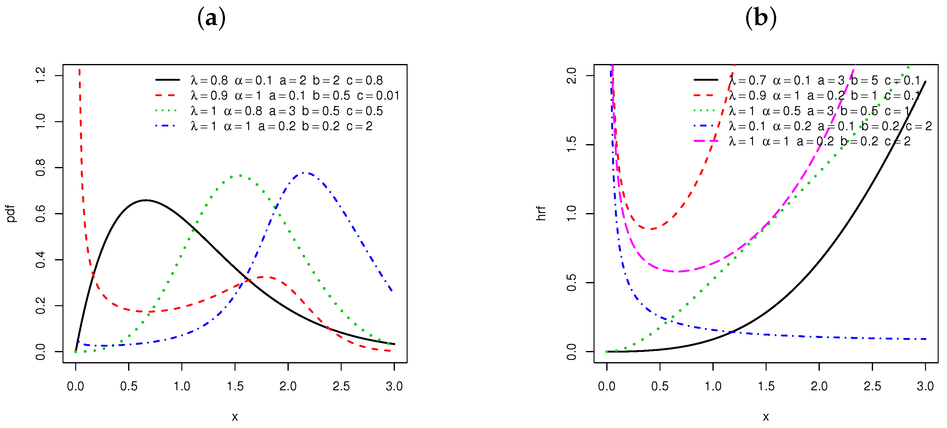
3.1. On the Shapes of the pdf
3.2. On the Shapes of the hrf
3.3. Linear Representation
3.4. Quantile Function
3.5. Moments
3.6. Skewness
3.7. Moment Generating Function
3.8. Incomplete Moments and Mean Deviations
3.9. Entropies
3.10. Order Statistics
4. Statistical Inference
4.1. Maximum Likelihood Estimation
4.2. Simulation
4.3. Applications
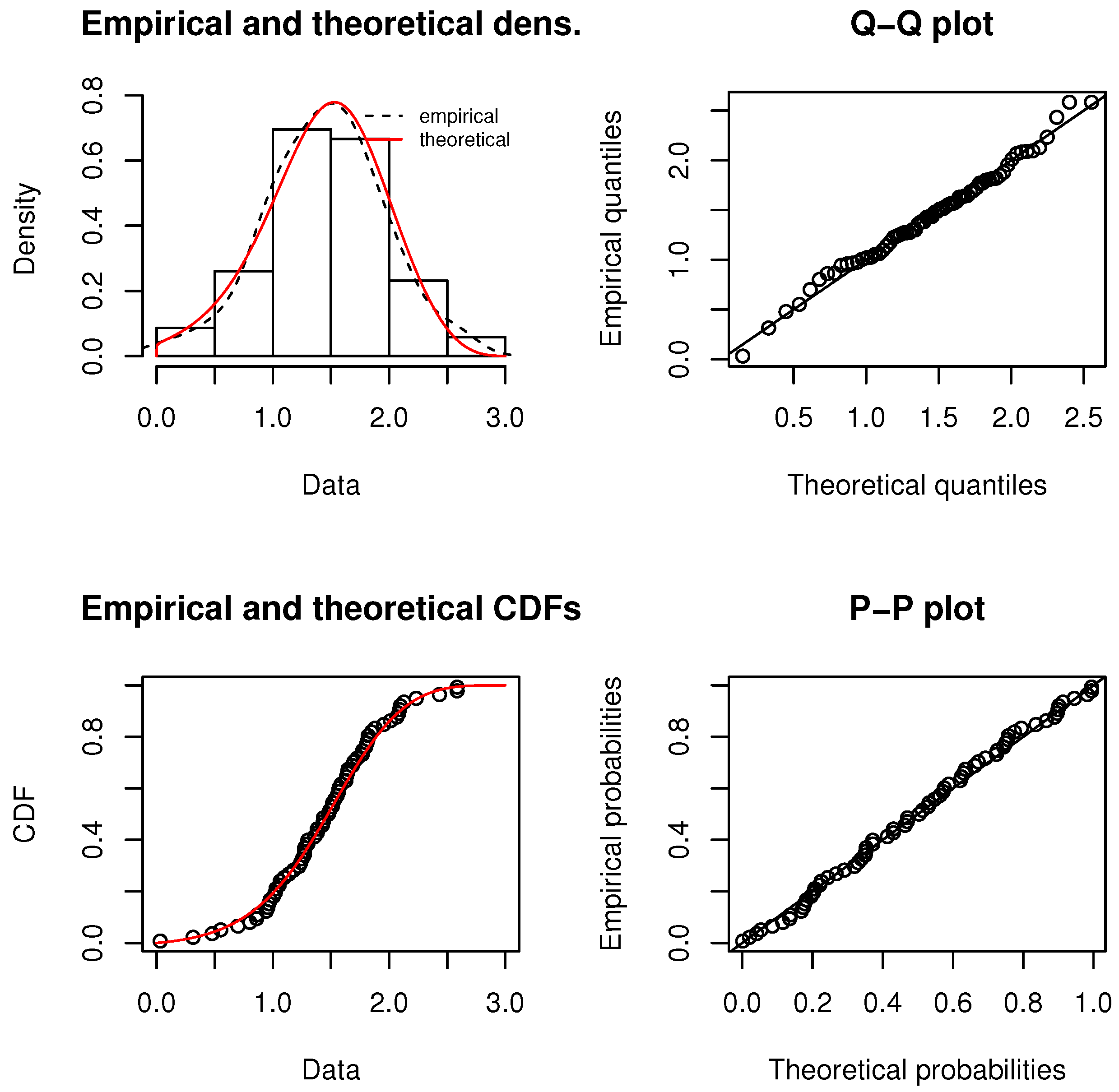
4.3.1. Dataset 1
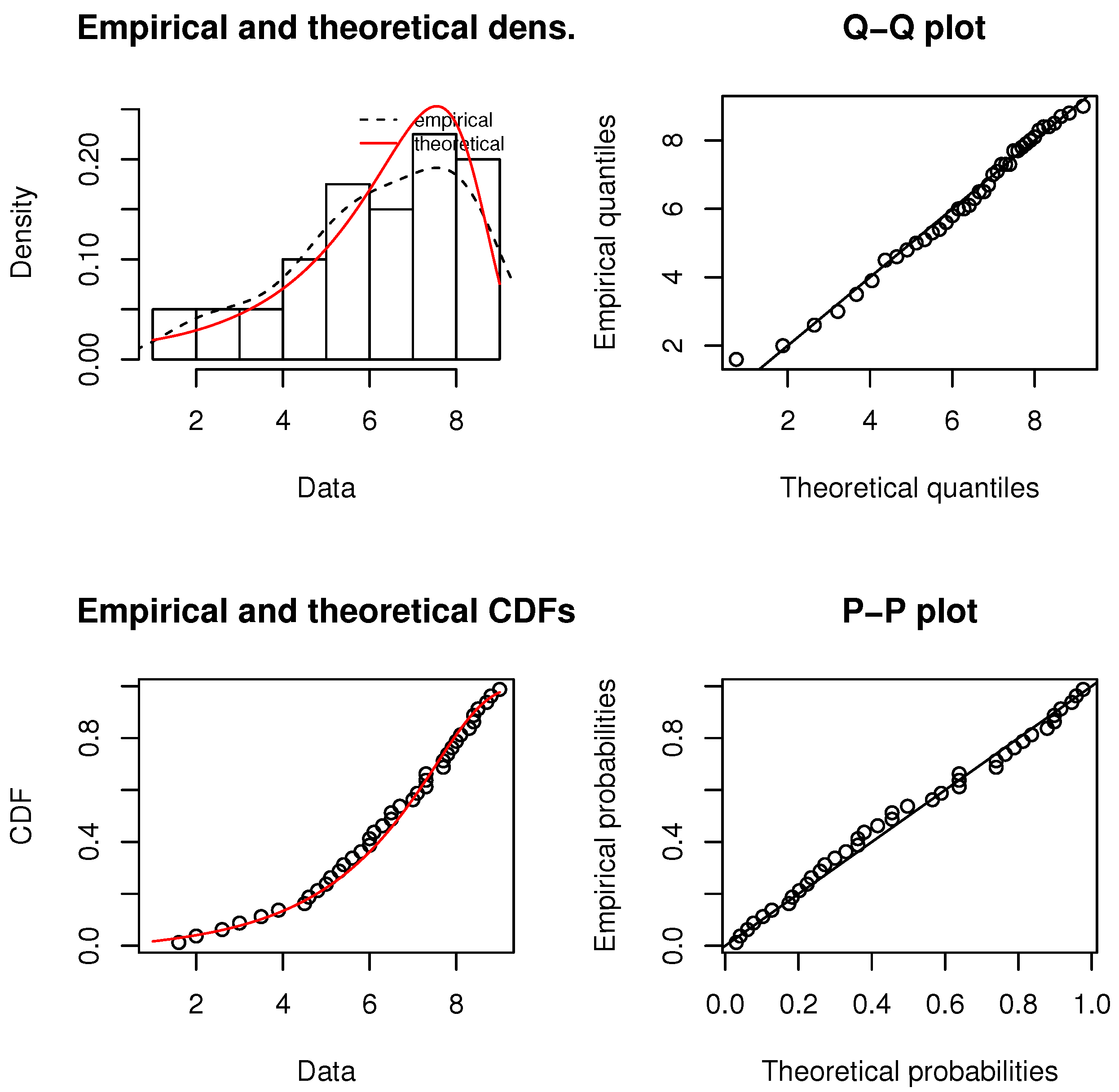
4.3.2. Dataset 2
Author Contributions
Funding
Acknowledgments
Conflicts of Interest
References
- Gompertz, B. On the nature of the function expressive of the law of human mortality and on the new mode of determining the value of life contingencies. Philos. Trans. R. Soc. A 1825, 115, 513–580. [Google Scholar] [CrossRef]
- Tjørve, K.M.C.; Tjørve, E. The use of Gompertz models in growth analyses, and new Gompertz-model approach: An addition to the Unified-Richards family. PLoS ONE 2017, 12. [Google Scholar] [CrossRef]
- El-Gohary, A.; Alshamrani, A.; Al-Otaibi, A. The generalized Gompertz distribution. Appl. Math. Model. 2013, 37, 13–24. [Google Scholar] [CrossRef]
- Jafari, A.A.; Tahmasebi, S.; Alizadeh, M. The beta-Gompertz distribution. Revista Colombiana de Estadistica 2014, 37, 141–158. [Google Scholar] [CrossRef]
- Eugene, N.; Lee, C.; Famoye, F. Beta-normal distribution and its applications. Comm. Statist. Theory Methods 2002, 31, 497–512. [Google Scholar] [CrossRef]
- Benkhelifa, L. The beta generalized Gompertz distribution. Appl. Math. Model. 2017, 52, 341–357. [Google Scholar] [CrossRef]
- El-Damcese, M.A.; Mustafa, A.; El-Desouky, B.S.; Mustafa, M.E. Generalized Exponential Gompertz Distribution. Appl. Math. 2015, 6, 2340–2353. [Google Scholar] [CrossRef]
- Tahir, M.H.; Cordeiro, G.M.; Alizadeh, M.; Mansoor, M.; Zubair, M.; Hamedani, G.G. The Odd Generalized Exponential Family of Distributions with Applications. J. Stat. Distrib. Appl. 2015, 2, 1–28. [Google Scholar] [CrossRef]
- Roozegar, R.; Tahmasebi, S.; Jafari, A.A. The McDonald Gompertz distribution: Properties and applications. Commun. Stat. Simul. Comput. 2017, 46, 3341–3355. [Google Scholar] [CrossRef]
- Alexander, C.; Cordeiro, G.M.; Ortega, E.M.M.; Sarabia, J.M. Generalized beta-generated distributions. Comput. Stat. Data Anal. 2012, 56, 1880–1897. [Google Scholar] [CrossRef]
- Khan, M.S.; King, R.; Hudson, I.L. Transmuted Generalized Gompertz distribution with application. J. Stat. Theory Appl. 2017, 16, 65–80. [Google Scholar] [CrossRef]
- Moniem, A.I.B.; Seham, M. Transmuted Gompertz Distribution. Comput. Appl. Math. 2015, 1, 88–96. [Google Scholar]
- Shaw, W.; Buckley, I. The Alchemy of Probability Distributions: Beyond Gram-Charlier Expansions and a Skewkurtotic-Normal Distribution from a Rank Transmutation Map; Research Report; King’s College: London, UK, 2007. [Google Scholar]
- Chukwu, A.U.; Ogunde, A.A. On kumaraswamy gompertz makeham distribution. Am. J. Math. Stat. 2016, 6, 122–127. [Google Scholar]
- Lima, F.P.; Sanchez, J.D.; da Silva, R.C.; Cordeiro, G.M. The Kumaraswamy Gompertz distribution. J. Data Sci. 2015, 13, 241–260. [Google Scholar]
- Benkhelifa, L. Marshall-Olkin extended generalized Gompertz distribution. J. Data Sci. 2017, 15, 239–266. [Google Scholar]
- Yaghoobzadeh, S. A new generalization of the Marshall-Olkin Gompertz distribution. Int. J. Syst. Assur. Eng. Manag. 2017, 8, 1580–1587. [Google Scholar] [CrossRef]
- Marshall, A.W.; Olkin, I. A new method for adding a parameter to a family of distributions with application to the exponential and Weibull families. Biometrika 1997, 84, 641–652. [Google Scholar] [CrossRef]
- Shadrokh, A.; Yaghoobzadeh, S.S. The Beta Gompertz Geometric Distribution: Mathematical Properties and Applications. Andishe_ye Amari 2018, 22, 81–91. [Google Scholar]
- Nadarajah, S.; Teimouri, M.; Shih, S.H. Modified Beta Distributions. Sankhya Ser. B 2014, 76, 19–48. [Google Scholar] [CrossRef]
- Alizadeh, M.; Cordeiro, G.M.; Brito, E. The beta Marshall-Olkin family of distributions. J. Stat. Distrib. Appl. 2015, 2, 4. [Google Scholar] [CrossRef]
- Nadarajah, S.; Kotz, S. The beta exponential distribution. Reliab. Eng. Syst. Saf. 2006, 91, 689–697. [Google Scholar] [CrossRef]
- Gupta, R.D.; Kundu, D. Generalized Exponential Distributions. Aust. N. Z. J. Stat. 1999, 41, 173–188. [Google Scholar] [CrossRef]
- Kenney, J.F.; Keeping, E.S. Mathematics of Statistics, 3rd ed.; Chapman and Hall Ltd.: Rahway, NJ, USA, 1962. [Google Scholar]
- Moors, J.J. A quantile alternative for kurtosis. J. R. Stat. Soc. Ser. D 1988, 37, 25–32. [Google Scholar] [CrossRef]
- Milgram, M. The generalized integro-exponential function. Math. Comput. 1985, 44, 443–458. [Google Scholar] [CrossRef]
- Lenart, A. The moments of the Gompertz distribution and maximum likelihood estimation of its parameters. Scand. Actuar. J. 2014, 3, 255–277. [Google Scholar] [CrossRef]
- MacGillivray, H.L. Skewness and Asymmetry: Measures and Orderings. Ann. Stat. 1986, 14, 994–1011. [Google Scholar] [CrossRef]
- Gradshteyn, I.S.; Ryzhik, I.M. Table of Integrals, Series and Products; Academic Press: New York, NY, USA, 2000. [Google Scholar]
- El-Bassiouny, H.; EL-Damcese, M.; Mustafa, A.; Eliwa, M.S. Exponentiated Generalized Weibull-Gompertz Distribution with Application in Survival Analysis. J. Stat. Appl. Probab. 2017, 6, 7–16. [Google Scholar] [CrossRef]
- Xu, K.; Xie, M.; Tang, L.C.; Ho, S.L. Application of Neural Networks in forecasting Engine Systems Reliability. Appl. Soft Comput. 2003, 2, 255–268. [Google Scholar] [CrossRef]
- Badar, M.G.; Priest, A.M. Statistical aspects of fiber and bundle strength in hybrid composites. In Progress in Science and Engineering Composites, Proceedings of the ICCM-IV, Tokyo, Japan, 25–28 October 1982; Hayashi, T., Kawata, K., Umekawa, S., Eds.; Japan Society for Composite Materials: Tokyo, Japan, 1982; pp. 1129–1136. [Google Scholar]


| n | Parameters | Initial | MLE | MSE | Initial | MLE | MSE |
|---|---|---|---|---|---|---|---|
| 50 | a | 3.0 | 3.0024 | 0.5057 | 2.5 | 2.6424 | 0.1737 |
| b | 1.5 | 1.6409 | 0.1499 | 1.5 | 1.5219 | 0.0400 | |
| c | 0.5 | 0.4941 | 0.0008 | 0.5 | 0.5050 | 0.0004 | |
| 0.5 | 0.5422 | 0.0198 | 0.5 | 0.5291 | 0.0116 | ||
| 0.5 | 0.5241 | 0.0387 | 0.5 | 0.5235 | 0.0122 | ||
| 100 | a | 3.0 | 3.0778 | 0.2458 | 2.5 | 2.5060 | 0.0754 |
| b | 1.5 | 1.6083 | 0.0779 | 1.5 | 1.5373 | 0.0291 | |
| c | 0.5 | 0.4986 | 0.0003 | 0.5 | 0.4991 | 0.0003 | |
| 0.5 | 0.5572 | 0.0147 | 0.5 | 0.5123 | 0.0029 | ||
| 0.5 | 0.4926 | 0.0126 | 0.5 | 0.5035 | 0.0070 | ||
| 150 | a | 3.0 | 2.9041 | 0.1015 | 2.5 | 2.5125 | 0.0284 |
| b | 1.5 | 1.6159 | 0.0485 | 1.5 | 1.5232 | 0.0088 | |
| c | 0.5 | 0.4940 | 0.0002 | 0.5 | 0.5002 | 0.0001 | |
| 0.5 | 0.5477 | 0.0094 | 0.5 | 0.5137 | 0.0015 | ||
| 0.5 | 0.4694 | 0.0072 | 0.5 | 0.4968 | 0.0015 | ||
| 50 | a | 1.5 | 1.4706 | 0.0325 | 1.5 | 1.5435 | 0.0641 |
| b | 1.8 | 1.7764 | 0.0639 | 1.8 | 1.7838 | 0.0955 | |
| c | 0.5 | 0.5054 | 0.0013 | 1.5 | 1.5285 | 0.0203 | |
| 0.5 | 0.4833 | 0.0029 | 0.5 | 0.4895 | 0.0008 | ||
| 0.5 | 0.5488 | 0.0160 | 0.5 | 0.5364 | 0.0118 | ||
| 100 | a | 1.5 | 1.5138 | 0.0201 | 1.5 | 1.5194 | 0.0224 |
| b | 1.8 | 1.8177 | 0.0380 | 1.8 | 1.8309 | 0.0451 | |
| c | 0.5 | 0.5004 | 0.0007 | 1.5 | 1.5010 | 0.0047 | |
| 0.5 | 0.5007 | 0.0023 | 0.5 | 0.5011 | 0.0005 | ||
| 0.5 | 0.5106 | 0.0059 | 0.5 | 0.5036 | 0.0028 | ||
| 150 | a | 1.5 | 1.5313 | 0.0102 | 1.5 | 1.4690 | 0.0094 |
| b | 1.8 | 1.8152 | 0.0194 | 1.8 | 1.8396 | 0.0258 | |
| c | 0.5 | 0.5055 | 0.0003 | 1.5 | 1.4864 | 0.0017 | |
| 0.5 | 0.5173 | 0.0022 | 0.5 | 0.5007 | 0.0004 | ||
| 0.5 | 0.5044 | 0.0034 | 0.5 | 0.4943 | 0.0009 |
| Distribution | Estimates | ||||
|---|---|---|---|---|---|
| MBGz () | 0.0085 | 2.5537 | 1.0737 | 1.3153 | 5.0687 |
| (0.0067) | (0.5727) | (0.3197) | (0.8933) | (3.3003) | |
| EGWGz () | 3.2078 | 2.4598 | 0.0203 | 1.8974 | 0.5460 |
| (1.2099) | (0.6498) | (0.0531) | (1.8193) | (0.2430) | |
| KwGz () | 0.1861 | 1.4948 | 1.4909 | 0.9811 | |
| (0.3130) | (0.5076) | (0.4735) | (2.4368) | ||
| BGz () | 0.3144 | 1.5591 | 1.4798 | 0.4966 | |
| (0.4283) | (0.3658) | (0.4543) | (0.8692) | ||
| Gz () | 0.0841 | 1.8811 | |||
| (0.0268) | (0.2043) |
| Distribution | Estimates | ||||
|---|---|---|---|---|---|
| MBGz () | 0.0098 | 0.5270 | 0.8768 | 4.5635 | 0.1561 |
| (0.0116) | (0.1599) | (0.3893) | (0.8862) | (0.2442) | |
| EGWGz () | 0.0101 | 0.6077 | 0.1078 | 1.6929 | 0.6613 |
| (0.0141) | (0.1506) | (0.3427) | (1.2539) | (0.3379) | |
| KwGz () | 0.0133 | 0.2923 | 2.0164 | 13.7085 | |
| (0.0120) | (0.1641) | (0.7880) | (7.0208) | ||
| BGz () | 0.0125 | 0.1856 | 3.7622 | 2.0116 | |
| (0.0100) | (0.1601) | (2.5635) | (3.3802) | ||
| Gz () | 0.0074) | (0.6243) | |||
| (0.0035) | (0.0748) |
| Dist | AIC | BIC | W* | A* | KS | p-Value | |
|---|---|---|---|---|---|---|---|
| MBGz | 50.0387 | 110.0776 | 118.2481 | 0.0328 | 0.2745 | 0.0539 | 0.9889 |
| EGWGz | 52.6888 | 115.3776 | 126.5482 | 0.0706 | 0.5341 | 0.0785 | 0.7885 |
| KwGz | 51.2042 | 110.4084 | 119.3448 | 0.0529 | 0.4125 | 0.0640 | 0.9396 |
| BGz | 51.1518 | 110.3026 | 119.2399 | 0.0518 | 0.4057 | 0.0627 | 0.9484 |
| Gz | 53.9686 | 111.9374 | 122.4056 | 0.0819 | 0.5921 | 0.0810 | 0.7547 |
| Dist | AIC | BIC | W* | A* | KS | p-Value | |
|---|---|---|---|---|---|---|---|
| MBGz | 78.2184 | 168.1770 | 176.0214 | 0.0222 | 0.1840 | 0.0707 | 0.9888 |
| EGWGz | 79.3744 | 168.5489 | 178.5933 | 0.0479 | 0.2922 | 0.0821 | 0.9623 |
| KwGz | 80.7197 | 169.4395 | 176.1950 | 0.0430 | 0.3326 | 0.0966 | 0.8489 |
| BGz | 82.9924 | 173.9849 | 180.7404 | 0.0922 | 0.6736 | 0.1080 | 0.7389 |
| Gz | 80.9566 | 168.9234 | 177.2911 | 0.0359 | 0.2335 | 0.0903 | 0.8299 |
© 2018 by the authors. Licensee MDPI, Basel, Switzerland. This article is an open access article distributed under the terms and conditions of the Creative Commons Attribution (CC BY) license (http://creativecommons.org/licenses/by/4.0/).
Share and Cite
Elbatal, I.; Jamal, F.; Chesneau, C.; Elgarhy, M.; Alrajhi, S. The Modified Beta Gompertz Distribution: Theory and Applications. Mathematics 2019, 7, 3. https://doi.org/10.3390/math7010003
Elbatal I, Jamal F, Chesneau C, Elgarhy M, Alrajhi S. The Modified Beta Gompertz Distribution: Theory and Applications. Mathematics. 2019; 7(1):3. https://doi.org/10.3390/math7010003
Chicago/Turabian StyleElbatal, Ibrahim, Farrukh Jamal, Christophe Chesneau, Mohammed Elgarhy, and Sharifah Alrajhi. 2019. "The Modified Beta Gompertz Distribution: Theory and Applications" Mathematics 7, no. 1: 3. https://doi.org/10.3390/math7010003
APA StyleElbatal, I., Jamal, F., Chesneau, C., Elgarhy, M., & Alrajhi, S. (2019). The Modified Beta Gompertz Distribution: Theory and Applications. Mathematics, 7(1), 3. https://doi.org/10.3390/math7010003