Abstract
Calculating nodal voltages and branch current flows in a meshed network is fundamental to electrical engineering. This work demonstrates how such calculations can be performed using the eigenvalues and eigenvectors of the Laplacian matrix which describes the connectivity of the electrical network. These insights should permit the functioning of electrical networks to be understood in the context of spectral analysis.
1. Introduction
Electrical power system calculations rely heavily on the bus admittance matrix, , which is a Laplacian matrix weighted by the complex-valued admittance of each branch in the network. It is well established that the eigenvalues and eigenvectors (deemed the spectrum) of a Laplacian matrix encode meaningful information about a network’s structure [1]. Recent work in [2,3] indicates that, in electrical networks, this spectrum can be directly related to nodal voltages and branch current flows. The purpose of the present paper is to clarify the derivations provided in [3]. The scope of the present work is narrowly theoretical: Linear algebra is used to articulate the correct relationship between the variables treated in [3].
Notwithstanding these modest ambitions, a key motivation for the present work is to begin to link power flow analysis with the mature literature [4] on spectral graph theory. Extant efforts to apply spectral graph theory to electrical networks are scarce, but include [5,6]. The use of graph theory more generally in this role is reviewed in [7,8]. Notably, simplistic topological approaches do not properly account for the physical realities of electrical power flow, and can thereby fail to identify the critical components in an electrical network [9,10,11]. The present work seeks to articulate one particular linkage between spectral graph theory and circuit theory, which may offer new ways to understand how power flows in meshed electrical networks.
2. Preliminaries
2.1. Electrical Flow Basics and Notation
Ohm’s law linearly relates the current flowing through an edge in a circuit with the voltage difference between the nodes that the edge connects. Specifically, , and , where is the current passing from the k-th node to the j-th in a (typically sparsely connected) network of N nodes, is the voltage difference between the k-th node and the j-th, is branch impedance and are complex-valued net current injections or withdrawals. From the above notation we arrive easily at i.e., , or, equivalently,
In the article we will denote with for the Kronecker delta, i.e., and for . With we will denote the complex conjugate of u, and with T, * the conjugate transpose, and conjugate transpose tensor respectively.
2.2. An Exemplary Electrical Network
To provide some context, a nation-spanning electrical power system is shown in Figure 1. This diagram of the nesta_case2224_edin test system [12] was created using the techniques described in [13], which uses electrical distances measures, rather than physical geography, to positions nodes. Note the relative spareseness of its connective struture, and how lower nominal voltage levels ( kV) correspond to more tree-like structures. This network of 2224 nodes supplies a total load of up to 60 GW, supplied from 378 different generating sites.
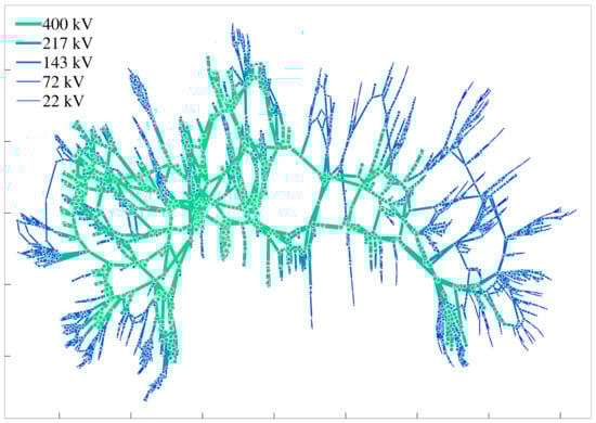
Figure 1.
This diagram shows the nesta_case2224_edin test power system
3. Derivations
In this section, first we rewrite (1) in matrix form and define the relevant Laplacian matrix. Then we provide a formula which explicitly relates the voltage differences to the eigenvalues and eigenvectors of the Laplacian matrix for meshed electrical networks. We can state now the following theorem.
Theorem 1.
Consider an electrical network with branch currents , passing from node k to node j, a complex impedance describing each branch , and being the complex-valued net current flow at each bus with . Then the voltage difference between two arbitrary nodes m and n is given by:
where , are the non-zero eigenvalues of the G matrix (equivalent to the matrix in the power systems context) which describes the connectivity of the electrical network:
and is an eigenvector of the eigenvalue .
Proof.
We arrive at . We observe that if , is an element of G, then for , and for , . Hence G is given by (3). We will refer to G as the Laplacian matrix. Note that the rows of G sum to zero, i.e., the matrix has the zero eigenvalue (see [3,14]). The algebraic multiplicity of the zero eigenvalue in the Laplacian is the number of connected components in the network. In the power systems case we deal with only one network which means the algebraic multiplicity of the zero eigenvalue is one. Since the matrix G is symmetric it can be written in the following form:
where , is the conjugate transpose of P such that is the identity matrix and D is the diagonal matrix . By applying the above expression into the system we get:
and since is the inverse of P we have:
or, equivalently,
Let be a column vector that contains exactly N 1’s. From the fact that every row of G sums to zero we have the eigenspace of the zero eigenvalue. Indeed which means that is the eigenspace of the zero eigenvalue. Hence there exist such that
From (4) , or, equivalently, . In addition, . Hence, . By ignoring the first row of each column of the above expression we get:
Which can be rewritten in the following form:
If we set , , we have
or, equivalently,
or, equivalently,
or, equivalently,
or, equivalently, for :
Let , be two arbitrary nodal voltages, i.e.,
Then, the difference between them is given by
or, equivalently,
or, equivalently,
□
4. Conclusions
This work has clarified the relationship between the admittance matrix spectrum, the current inflows & withdrawals prevailing in an electrical network and the resulting nodal voltage profile. Applying these spectral relationships to practical electrical engineering problems is left to future work.
Author Contributions
Methodology, I.D.; Formal Analysis, I.D.; P.C.; A.K.; Writing—Original Draft Preparation, I.D.; Writing—Review and Editing, I.D.; P.C.; Visualization, P.C.; Supervision, P.C.; A.K.
Funding
This material is supported by the Science Foundation Ireland (SFI), by funding Ioannis Dassios under Investigator Programme Grant No. SFI/15/IA/3074; and A. Keane and P. Cuffe under the SFI Strategic Partnership Programme Grant Number SFI/15/SPP/E3125. The opinions, findings and conclusions or recommendations expressed in this material are those of the authors and do not necessarily reflect the views of the Science Foundation Ireland.
Conflicts of Interest
The authors declare no conflict of interest.
References
- Mohar, B.; Alavi, Y.; Chartrand, G.; Oellermann, O. The Laplacian spectrum of graphs. Graph Theory Comb. Appl. 1991, 2, 12. [Google Scholar]
- Rubido, N.; Grebogi, C.; Baptista, M.S. Structure and function in flow networks. EPL (Europhys. Lett.) 2013, 101, 68001. [Google Scholar] [CrossRef]
- Rubido, N.; Grebogi, C.; Baptista, M.S. General analytical solutions for DC/AC circuit-network analysis. Eur. Phys. J. Spec. Top. 2017, 226, 1829–1844. [Google Scholar] [CrossRef]
- Chung, F.R.; Graham, F.C. Spectral Graph Theory; Number 92; American Mathematical Society: Providence, RI, USA, 1997. [Google Scholar]
- Edström, F. On eigenvalues to the Y-bus matrix. Int. J. Electr. Power Energy Syst. 2014, 56, 147–150. [Google Scholar] [CrossRef]
- Edström, F.; Söder, L. On spectral graph theory in power system restoration. In Proceedings of the 2011 2nd IEEE PES International Conference and Exhibition on Innovative Smart Grid Technologies (ISGT Europe), Manchester, UK, 5–7 December 2011; pp. 1–8. [Google Scholar]
- Pagani, G.A.; Aiello, M. The power grid as a complex network: A survey. Phys. A Stat. Mech. Its Appl. 2013, 392, 2688–2700. [Google Scholar] [CrossRef]
- Sun, K. Complex networks theory: A new method of research in power grid. In Proceedings of the 2005 IEEE/PES Transmission and Distribution Conference and Exhibition: Asia and Pacific, Dalian, China, 18 August 2005; pp. 1–6. [Google Scholar]
- Hines, P.; Cotilla-Sanchez, E.; Blumsack, S. Do topological models provide good information about electricity infrastructure vulnerability? Chaos Interdiscip. J. Nonlinear Sci. 2010, 20, 033122. [Google Scholar] [CrossRef] [PubMed]
- Verma, T.; Ellens, W.; Kooij, R.E. Context-independent centrality measures underestimate the vulnerability of power grids. arXiv, 2013; arXiv:1304.5402. [Google Scholar]
- Cuffe, P. A comparison of malicious interdiction strategies against electrical networks. IEEE J. Emerg. Sel. Top. Circuits Syst. 2017, 7, 205–217. [Google Scholar] [CrossRef]
- Coffrin, D.; Gordon, D.; Scott, P. Nesta the nicta energy system test case archive. arXiv, 2014; arXiv:1411.0359. [Google Scholar]
- Cuffe, P.; Keane, A. Visualizing the electrical structure of power systems. IEEE Syst. J. 2017, 11, 1810–1821. [Google Scholar] [CrossRef]
- Dassios, I.K.; Cuffe, P.; Keane, A. Visualizing voltage relationships using the unity row summation and real valued properties of the FLG matrix. Electr. Power Syst. Res. 2016, 140, 611–618. [Google Scholar] [CrossRef]
© 2019 by the authors. Licensee MDPI, Basel, Switzerland. This article is an open access article distributed under the terms and conditions of the Creative Commons Attribution (CC BY) license (http://creativecommons.org/licenses/by/4.0/).