Fractional Metric Dimension of Generalized Jahangir Graph

Abstract

Arumugam and Mathew [Discret. Math. 2012, 312, 1584–1590] introduced the notion of fractional metric dimension of a connected graph. In this paper, a combinatorial technique is devised to compute it. In addition, using this technique the fractional metric dimension of the generalized Jahangir graph $J_{m,k}$ is computed for $k\ge 0$ and $m=5$.

1. Introduction and Preliminaries

In this paper, $G=(V(G),E(G))$ is a finite, undirected, connected and simple graph of order $|V(G)|$ and size $|E(G)|$. For any two vertices $u,v\in V(G)$, the distance $d(u,v)$ is the length of a shortest path $u~v$ in G. For graph theoretic terminology, we refer to [1,2,3].

An ordered set of vertices, we mean a set $W=\{w_1,w_2,\cdots ,w_k\}$ on which the ordering $(w_1,w_2,\cdots ,w_k)$ has been imposed. For an ordered subset $W=\{w_1,w_2,\cdots ,w_k\}$ of $V(G)$, we refer to the $k$-vector (ordered $k$-tuple) $r(v|W)=(d(v,w_1),d(v,w_2),\cdots ,d(v,w_k))$ as the (metric) representation of v with respect to W. The set W is called a resolving set for G if $r(u|W)=r(v|W)$ implies that $u=v$ for all $u,v\in V(G)$. Hence, if W is a resolving set of cardinality k for a graph G of order n, then the set $\{r(v|W):v\in V(G)\}$ consists of n distinct $k$-vectors. A vertex $x\in V(G)$ is said to resolve $\{u,v\}\subseteq V(G)$ in G if $d(u,x)\ne d(v,x)$. The collection of all such x in $V(G)$ is called resolving neighbourhood of the pair $\{u,v\}$, denoted by $R\{u,v\}$. Explicitly, $R\{u,v\}=\{x\in V(G):d(u,x)\ne d(v,x)\}$. Let $V_p$ denote the collection of all $\left(\genfrac{}{}{0pt}{}{|V(G)|}{2}\right)$ pairs of vertices of G. Then for each $x\in V(G)$ the set $R\{x\}=\{\{u,v\}\in V_p:d(u,x)\ne d(v,x)\}$ is called resolvent neighbourhood of x.

Definition 1

([4]). Let $G=(V(G),E(G))$ be a connected graph of order n. A function $f:V(G)\to [0,1]$ is called a resolving function (RF) of G if $f(R\{u,v\})\ge 1$ for any two distinct vertices $u,v\in V(G)$, where $f(R\{u,v\})={\displaystyle \sum _{x\in R\{u,v\}}}f(x)$. A resolving function g of a graph G is minimal (MRF) if any function $f:V(G)\to [0,1]$ such that $f\le g$ and $f(v)\ne g(v)$ for at least one $v\in V(G)$ is not a resolving function of G. Then, the fractional metric dimension of the graph G is ${dim}_f(G)=min\{|g|:gis a minimal resolving function of G\},$ where $|g|={\displaystyle \sum _{v\in V(G)}}g(v).$

In [5,6], Slatter introduced the notion of resolving set of a connected graph under the term locating set. Harary and Melter in [7], independently discovered these concepts and termed them as the metric dimension of graph. Resolving sets enjoy their several applications in various areas of computer sciences such as network discovery and verification [8], robot navigation [9], mastermind game [10], coin weighing problem [11], integer programming [12] and drug discovery [13]. The problem of finding metric dimension of a graph as an integer programming problem (IPP) has been introduced by Chartrand et al. [13], and independently by Currie and Oellermann [12]. As a further refinement, Currie and Oellermann [8] devised the notion of fractional metric dimension as the optimal solution of the linear relaxation of the IPP. An equivalent formulation for the fractional metric dimension of a graph has been proposed by Fehr et al. [14] as follows:

Suppose $V=\{v_1,v_2,\dots ,v_n\}$ and $V_p=\{s_1,s_2,\dots ,s_{\left(\genfrac{}{}{0pt}{}{n}{2}\right)}\}$. Let $A=(a_{ij})$ be the $\left(\genfrac{}{}{0pt}{}{n}{2}\right)$ $\times n$ matrix with $a_{ij}=1$ if $s_i{v}_j\in E(R(G))$ and 0 otherwise, where $1\le i\le$ $\left(\genfrac{}{}{0pt}{}{n}{2}\right)$ and $1\le j\le n$. The IPP of the metric dimension is given by;

Minimize $f(x_1,x_2,\dots ,x_n)=x_1+x_2+,\dots ,+x_n$ subject to $A\overline{x}\ge \overline{1}$, where $\overline{x}={(x_1,x_2,\cdots ,x_n)}^T$, $x_i\in \{0,1\}$ and $\overline{1}$ is the $\left(\genfrac{}{}{0pt}{}{n}{2}\right)$ $\times 1$ column vector with all entries as 1.

The optimal solution of the aforementioned linear programming relaxation, with replacement $x_i\in \{0,1\}$ by $0\le x_i\le 1$ gives the fractional metric dimension of G, represented by ${dim}_f(G)$. The optimal solution of the dual of this LPP is referred to as the metric independence number of G$(m{i}_f(G))$. Therefore, the duality and weak duality theorem in linear programming implies that $mi(G)\le mif(G)={dim}_f(G)\le dim(G)$, as discussed by Arumugam and Mathew in [4]. For further details of the duality and weak duality theorem, we refer to [15].

In [16], Ali et al. introduced the generalized Jahangir graph as follows:

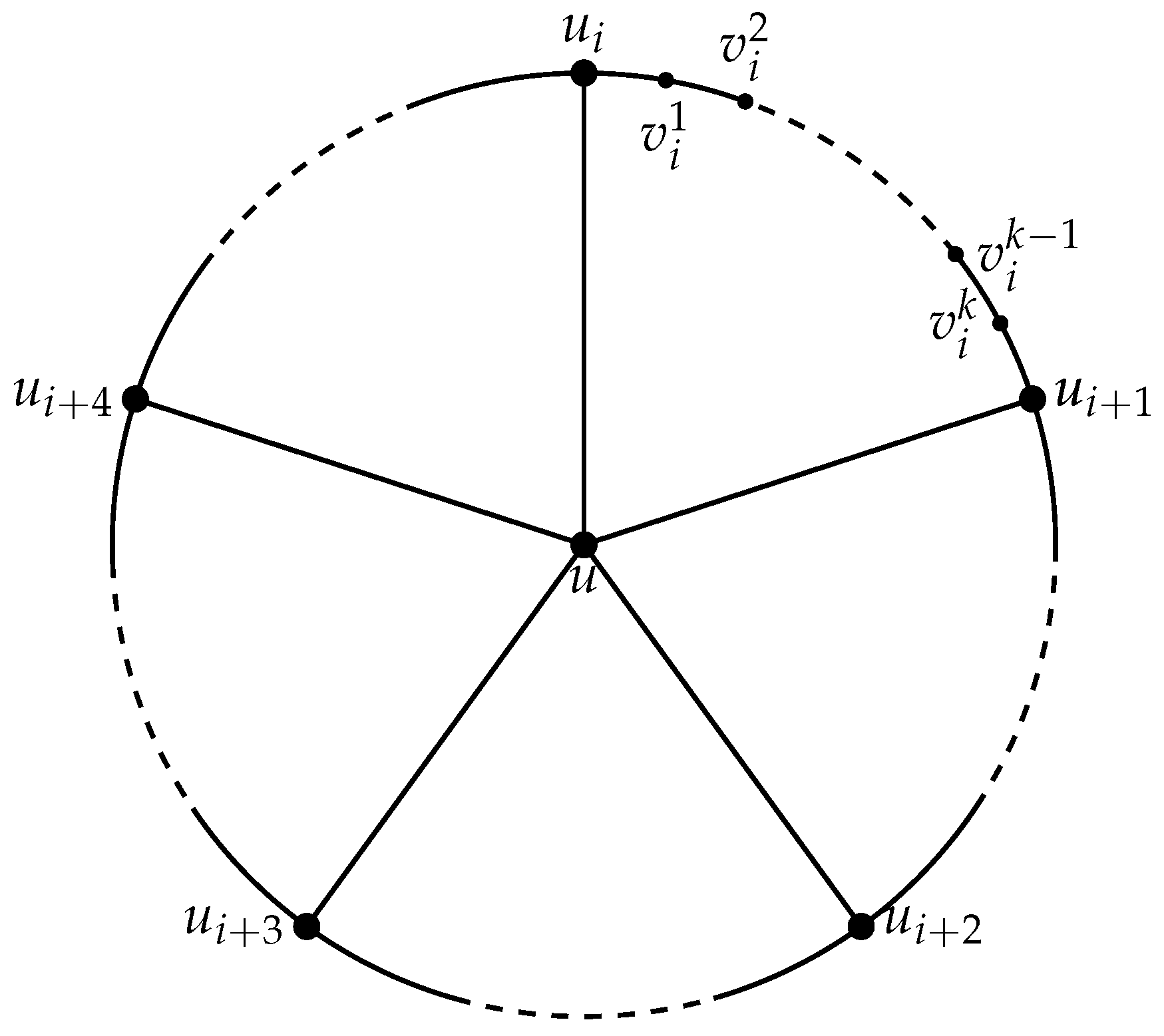
Definition 2.

The generalized Jahangir graph $J_{m,k}$, for $m\ge 3,k\ge 1$, is a graph on $m(k+1)+1$ vertices i.e., a graph consisting of a cycle $C_{m(k+1)}$ with one additional vertex which is adjacent to m vertices of $C_{m(k+1)}$ at distance $k+1$ to each other on $C_{m(k+1)}$. The vertex set of $J_{m,k}$ is $V(J_{m,k})=\{u,u_0,u_1,\dots ,u_{m-1}\}\bigcup \{v_i^1,v_i^2,\dots ,v_i^k|i=0,1,\dots ,m-1\}$ with $|V(J_{m,k})|=n=m(k+1)+1.$

The vertices of the generalized Jahangir graph $J_{m,k}$ can be classified into three different types. The vertices of degree $2,3$ and m are respectively named as minors, major and center. The generalized Jahangir graph $J_{m,k}$ have $km$ minor vertices, m major vertices and one center vertex. In this article, we have discussed results for $m=5$, shown in Figure 1. For $k=1$, the generalized Jahangir graph $J_{m,k}$ is the Jahangir graph $J_{2m}$, for $m\ge 4$, discussed by Tomescu et al. in [17].

Arumugam and Mathew [4] formally introduced the notion of fractional metric dimension and discussed some fundamental results. The fractional metric dimension of the cartesian product, hierarchical product, corona product, lexicographic product and comb product of connected graphs, see [18,19,20,21]. YI [22] computed the fractional metric dimension of permutation graphs. Mainly, Arumugama et al. [4] studied the graphs whose fractional metric dimension graphs equals half of their orders and Feng et al. [23] investigated the fractional metric dimension of vertex transitive and distance regular graphs. This motivated us to devise a criterion to compute fractional metric dimension of those graphs which are neither vertex transitive and distance regular graphs nor their fractional metric dimension is half of their orders. In particular, the criterion is applied to compute fractional metric dimension of the generalized Jahangir graph $J_{m,k}$ for $k\ge 0$ and $m=5$.

The paper is organized as follows: Section 1 is for introduction and preliminaries and in Section 2, the resolving neighbourhood of each possible pair of the vertices of the generalized Jahangir graph $J_{m,k}$ for $k\ge 0$ and $m=5$ are obtained. The main results are included in Section 3. Finally, the paper is concluded with some future prospects in Section 4.

2. Resolving Neighbourhoods of the Generalized Jahangir Graph ${\mathit{J}}_{\mathit{m},\mathit{k}}$ for $\mathit{k}\ge \mathbf{0}$ and $\mathit{m}=\mathbf{5}$

The possible pairs of vertices of the generalized Jahangir graph $J_{m,k}$ for $k\ge 1$ and $m=5$ are majors with majors, major with minors, center with majors, center with minors, and minors with minors. In this section, the resolving neighbourhoods for each pair of vertices of $J_{m,k}$ $k\ge 0$ and $m=5$ are classified.

Lemma 1.

Let $J_{m,k}$ be the generalized Jahangir graph for $k\ge 4$ and $m=5$. Then

$$|R_i|=|R\{v_{i-1}^k,v_i^1\}|=\left\{\begin{array}{ccc}\hfill k+4& if& k\equiv 0(mod2)\hfill \\ \hfill k+3& if& k\equiv 1(mod2).\hfill \end{array}\right.$$

Moreover, ${\cup }_{i=0}^4{R}_i=\{v_i^1,v_i^2,\dots ,v_i^k|i=0,1,\dots ,m-1\}$ and $\acute{\beta }=|{\cup }_{i=0}^4{R}_i|=5k$.

Proof. 

The resolving neighborhood of $\{v_{i-1}^k,v_i^1\}$ for $k\equiv 0(\mathrm{mod}2)$ is $R\{v_{i-1}^k,v_i^1\}=\{v_{i-1}^j|\frac{k}{2}-1\le j\le k\}\bigcup \{v_i^j|1\le j\le \frac{k}{2}+2\}$ with $|R_i|=k+4$. Similarly, the resolving neighborhood of $\{v_{i-1}^k,v_i^1\}$ for $k\equiv 1(\mathrm{mod}2)$ is $R\{v_{i-1}^k,v_i^1\}=\{v_{i-1}^j|\frac{k-1}{2}\le j\le k\}\bigcup \{v_i^j|1\le j\le \frac{k-1}{2}+2\}$ with $|R_i|=k+3$.

Also in both cases, ${\cup }_{i=0}^4{R}_i=\{v_i^1,v_i^2,\dots ,v_i^k|i=0,1,\dots ,m-1\}$ and hence $\acute{\beta }=|{\cup }_{i=0}^4{R}_i|=5k$. □

In the following lemma resolving neighbourhoods of the center vertex with major vertices in $J_{5,k}$ are computed.

Lemma 2.

Let $J_{m,k}$ be the generalized Jahangir graph for $k\ge 4$ and $m=5$. Then $|R_i|<|R\{u,u_i\}|$ and $|R\{u,u_i\}\cap ({\cup }_{i=0}^4{R}_i)|\ge |R_i|$.

Proof. 

For $k\equiv 0(\mathrm{mod}2)$, the resolving neighbourhood $R\{u,u_i\}$ is $V(J_{5,k})-\{v_{i-1}^{\frac{k}{2}},v_i^{\frac{k}{2}+1}\}$ with $|R\{u,u_i\}|=5k+4>k+4=|R_i|$ and $R\{u,u_i\}\cap ({\cup }_{i=0}^4{R}_i)={\cup }_{i=0}^4{R}_i)-\{v_{i-1}^{\frac{k}{2}},v_i^{\frac{k}{2}+1}\}$. Therefore, $|R\{u,u_i\}\cap ({\cup }_{i=0}^4{R}_i)|=5k-2>|R_i|$. Similarly, for $k\equiv 1(\mathrm{mod}2)$, $R\{u,u_i\}=V(J_{5,k})$ with $|R\{u,u_i\}|=n>k+3=|R_i|$ and $R\{u,u_i\}\cap ({\cup }_{i=0}^4{R}_i)={\cup }_{i=0}^4{R}_i)$. Therefore, $|R\{u,u_i\}\cap ({\cup }_{i=0}^4{R}_i)|=5k=|R_i|$. This completes the proof. □

In the following lemma resolving neighbourhoods of center vertex with minor vertices in $J_{5,k}$ are computed.

Lemma 3.

Let $J_{m,k}$ be the generalized Jahangir graph for $k\ge 4$ and $m=5$. Then $|R_i|<|R\{u,v_i^j\}|$ and $|R\{u,v_i^j\}\cap ({\cup }_{i=0}^4{R}_i)|\ge |R_i|$.

Proof. 

 

Case 1: (When $k\equiv 0(\mathrm{mod}2)$)

Since, $R\{u,v_i^1\}=V(J_{5,k})-\{v_{i-1}^{k-t}|0\le t\le \frac{k}{2}-1\}\bigcup \{u_i\}$ with $|R\{u,v_i^1\}|=4k+\frac{k}{2}+5>k+4=|R_i|$ and $R\{u,v_i^1\}\cap ({\cup }_{i=0}^4{R}_i)={\cup }_{i=0}^4{R}_i-\{v_{i-1}^{k-t}|0\le t\le \frac{k}{2}-1\}.$ Therefore, $|R\{u,v_i^1\}\cap ({\cup }_{i=0}^4{R}_i)|=4k+\frac{k}{2}$. Now for $1\le j\le \frac{k}{2}$, the resolving neighbourhood $R(u,v_i^j)=V(J_{5,k})-\{v_i^{\frac{k-4}{2}}\}$ with $|R\{u,v_i^j\}|=5k+5>k+4=|R_i|$. Also, $R\{u,v_i^j\}\cap ({\cup }_{i=0}^4{R}_i)={\cup }_{i=0}^4{R}_i-\{v_i^{\frac{k-4}{2}}\}$ and therefore, $|R\{u,v_i^j\}\cap ({\cup }_{i=0}^4{R}_i)|=5k+5>|R_i|$.

Case 2: (When $k\equiv 1(\mathrm{mod}2)$)

Since, $R\{u,v_i^1\}=V(J_{5,k})-\{v_{i-1}^t|\frac{k+1}{2}\le t\le k\}\bigcup \{u_i,v_i^{\frac{k+3}{2}}\}$ with $|R\{u,v_i^1\}|=3k+\frac{3k+1}{2}+3>k+3=|R_i|$ and $R\{u,v_i^1\}\cap ({\cup }_{i=0}^4{R}_i)={\cup }_{i=0}^4{R}_i-\{v_{i-1}^t|\frac{k+1}{2}\le t\le k\}\bigcup \{v_i^{\frac{k+3}{2}}\}$. Therefore, $|R\{u,v_i^1\}\cap ({\cup }_{i=0}^4{R}_i)|=4k+\frac{k-1}{2}-1>|R_i|$. Now for $3\le j\le \lceil \frac{k}{2}\rceil \&j$ is odd, the resolving neighbourhood $R(u,v_i^j)=V(J_{5,k})-\{v_i^{\frac{k+1}{2}},v_i^{\frac{k+5}{2}}\}$ with $|R\{u,v_i^j\}|=5k+4>k+3=|R_i|$. Also, $R\{u,v_i^j\}\cap ({\cup }_{i=0}^4{R}_i)={\cup }_{i=0}^4{R}_i-\{v_i^{\frac{k+1}{2}},v_i^{\frac{k+5}{2}}\}$ and therefore, $|R\{u,v_i^j\}\cap ({\cup }_{i=0}^4{R}_i)|=5k-2>|R_i|$. Finally, for $2\le j\le \lceil \frac{k}{2}\rceil \&j$ is even, $R\{u,v_i^j\}=V(J_{5,k})$, and the case is easy to see. This completes the proof. □

In the following lemma resolving neighbourhoods of the pair of major vertices in $J_{5,k}$ are computed.

Lemma 4.

Let $J_{m,k}$ be the generalized Jahangir graph for $k\ge 4$ and $m=5$. Then $|R_i|<|R\{u_i,u_{i+p}\}|$ and $|R\{u_i,u_{i+p}\}\cap ({\cup }_{i=0}^4{R}_i)|\ge |R_i|$ for $p=1,2$.

Proof. 

The symmetry of the generalized Jahangir graph $J_{5,k}$ allows us to discuss only the following case:

Case 1: (When $k\equiv 0(\mathrm{mod}2)$ and $p=1$)

Since, $R\{u_i,u_{i+1}\}=V(J_{5,k})-\{u,u_{i+2},u_{i+3},u_{i+4}\}\bigcup \{v_{i+1}^r,v_{i+2}^s,v_{i+3}^s,v_{i+4}^t,|\frac{k+4}{2}\le r\le k,1\le s\le k,1\le t\frac{k-2}{2}\}$ with $|R\{u_i,u_{i+1}\}|=2(k+2)>k+4=|R_i|$ and $R\{u_i,u_{i+1}\}\cap ({\cup }_{i=0}^4{R}_i)={\cup }_{i=0}^4{R}_i-\{v_{i+1}^r,v_{i+2}^s,v_{i+3}^s,v_{i+4}^t,|\frac{k+4}{2}\le r\le k,1\le s\le k,1\le t\le \frac{k-2}{2}\}$. Therefore, $|R\{u_i,u_{i+1}\}\cap ({\cup }_{i=0}^4{R}_i)|=2k+2>|R_i|$.

Case 2: (When $k\equiv 1(\mathrm{mod}2)$ and $p=1$)

Since, $R\{u_i,u_{i+1}\}=V(J_{5,k})-\{u,u_{i+2},u_{i+3},u_{i+4}\}\bigcup \{v_i^{\frac{k+1}{2}},v_{i+1}^r,v_{i+2}^s,v_{i+3}^s,v_{i+4}^t,|\frac{k+3}{2}\le r\le k,1\le s\le k,1\le t\le \frac{k-1}{2}\}$ with $|R\{u_i,u_{i+1}\}|=2(k+1)>k+4=|R_i|$ and $R\{u_i,u_{i+1}\}\cap ({\cup }_{i=0}^4{R}_i)={\cup }_{i=0}^4{R}_i-\{v_i^{\frac{k+1}{2}},v_{i+1}^r,v_{i+2}^s,v_{i+3}^s,v_{i+4}^t,|\frac{k+3}{2}\le r\le k,1\le s\le k,1\le t\le \frac{k-1}{2}\}$. Therefore, $|R\{u_i,u_{i+1}\}\cap ({\cup }_{i=0}^4{R}_i)|=2k>|R_i|$.

Case 3: (When $k\equiv 0(\mathrm{mod}2)$ and $p=2$)

Since, $R\{u_i,u_{i+2}\}=V(J_{5,k})-\{u,u_{i+1},u_{i+3},u_{i+4}\}\bigcup \{v_i^r,v_{i+1}^s,v_{i+2}^r,v_{i+3}^t,v_{i+4}^s|\frac{k+4}{2}\le r\le k,1\le s\le \frac{k-2}{2},1\le t\le k\}$ with $|R\{u_i,u_{i+2}\}|=2(k+3)>k+4=|R_i|$ and $R\{u_i,u_{i+2}\}\cap ({\cup }_{i=0}^4{R}_i)={\cup }_{i=0}^4{R}_i-\{v_i^r,v_{i+1}^s,v_{i+2}^r,v_{i+3}^t,v_{i+4}^s|\frac{k+4}{2}\le r\le k,1\le s\le \frac{k-2}{2},1\le t\le k\}$. Therefore, $|R\{u_i,u_{i+2}\}\cap ({\cup }_{i=0}^4{R}_i)|=2(k+2)>|R_i|$.

Case 4: (When $k\equiv 1(\mathrm{mod}2)$ and $p=0$)

Since, $R\{u_i,u_{i+2}\}=V(J_{5,k})-\{u,u_{i+1},u_{i+3},u_{i+4}\}\bigcup \{v_i^r,v_{i+1}^s,v_{i+2}^r,v_{i+3}^t,v_{i+4}^s|\frac{k+3}{2}\le r\le k,1\le s\le \frac{k-1}{2},1\le t\le k\}$ with $|R\{u_i,u_{i+2}\}|=2(k+2)>k+4=|R_i|$ and $R\{u_i,u_{i+2}\}\cap ({\cup }_{i=0}^4{R}_i)={\cup }_{i=0}^4{R}_i-\{v_i^r,v_{i+1}^s,v_{i+2}^r,v_{i+3}^t,v_{i+4}^s|\frac{k+3}{2}\le r\le k,1\le s\le \frac{k-1}{2},1\le t\le k\}$. Therefore, $|R\{u_i,u_{i+2}\}\cap ({\cup }_{i=0}^4{R}_i)|=2(k+1)>|R_i|$. □

In the following lemma resolving neighbourhoods of major vertices with minor vertices in $J_{5,k}$ are computed.

Lemma 5.

Let $J_{m,k}$ be the generalized Jahangir graph for $k\ge 4$ and $m=5$. Then $|R_i|<|R\{u_i,v_{i+p}^j\}|$ and $|R\{u_i,v_{i+p}^j\}\cap ({\cup }_{i=0}^4{R}_i)|\ge |R_i|$ for $p=0,1,2$.

Proof. 

 

Case 1: (When $k\equiv 0(\mathrm{mod}2)$ and $p=0$)

For $1\le j\le k-2$, the resolving neighbourhood $R\{u_i,v_i^j\}=V(J_{5,k})-\{v_i^{\frac{j}{2}}\}$ and $R\{u_i,v_i^j\}=V(J_{5,k})-\{v_i^{\frac{k+j+3}{2}}\}$ for j is even and odd respectively. Also, $|R\{u_i,v_i^j\}|=5k+5>k+4>|R_i|$ and $|R\{u_i,v_i^j\}\cap ({\cup }_{i=0}^4{R}_i)|=5k-1>|R_i|$. Now $R\{u_i,v_i^{k-1}\}=V(J_{5,k})-\{u_{i+1},v_{i+1}^j|1\le j\le \frac{k}{2}\}$ and $R\{u_i,v_i^k\}=V(J_{5,k})-\{v_i^{\frac{k}{2}},v_{i+1}^{\frac{k}{2}+1}\}$, therefore, $|R\{u_i,v_i^{k-1}\}|=\frac{9k+10}{2}>|R_i|$, $|R\{u_i,v_i^k\}|=5k+4>|R_i|$, $|R\{u_i,v_i^{k-1}\}\cap ({\cup }_{i=0}^4{R}_i)|=5k-\frac{k}{2}>|R_i|$ and $|R\{u_i,v_i^k\}\cap ({\cup }_{i=0}^4{R}_i)|=5k-2>|R_i|$.

Case 2: (When $k\equiv 0(\mathrm{mod}2)$ and $p=1$)

In this case, the resolving neighbourhoods are $R\{u_i,v_{i+1}^1\}=V(J_{5,k})-\{v_i^{\frac{k}{2}+1},v_{i+1}^{\frac{k+4}{2}}\}$, $R\{u_i,v_{i+1}^2\}=V(J_{5,k})-\{u_i,v_i^j|\frac{k+4}{2}\le j\le k\}$, $R{\{u_i,v_{i+1}^j\}}_{j=3}^{k-2}=V(J_{5,k})-\{v_{i+1}^{\frac{j-2}{2}}\}$ for even j, $R{\{u_i,v_{i+1}^j\}}_{j=3}^{k-2}=V(J_{5,k})-\{v_{i+1}^{\frac{k+j+3}{2}}\}$ for odd j, $R\{u_i,v_i^{k-1}\}=V(J_{5,k})-\{u_{i+2},v_{i+2}^j|1\le j\le \frac{k}{2}\}$ and $R\{u_i,v_i^k\}=V(J_{5,k})-\{v_{i+1}^{\frac{k}{2}-1},v_{i+2}^{\frac{k}{2}+1}\}$. Therefore, $|R{\{u_i,v_{i+1}^j\}}_{j=3}^{k-2}|=5k+5>5k+4=|R\{u_i,v_{i+1}^1\}|=|R\{u_i,v_i^k\}|>4k+\frac{k}{2}+6=|R\{u_i,v_{i+1}^2\}|>4k+\frac{k}{2}+5=|R\{u_i,v_i^{k-1}\}|>k+4=|R_i|$. Also, $|R{\{u_i,v_{i+1}^j\}}_{j=3}^{k-2}\cap ({\cup }_{i=0}^4{R}_i)|=5k-1>5k-2=|R\{u_i,v_{i+1}^1\}\cap ({\cup }_{i=0}^4{R}_i)|=|R\{u_i,v_{i+1}^k\}\cap ({\cup }_{i=0}^4{R}_i)|>4k+\frac{k}{2}+1=|R\{u_i,v_{i+1}^2\}\cap ({\cup }_{i=0}^4{R}_i)|>4k+\frac{k}{2}=|R\{u_i,v_{i+1}^{k-1}\}\cap ({\cup }_{i=0}^4{R}_i)|>|R_i|$.

Case 3: (When $k\equiv 0(\mathrm{mod}2)$ and $p=2$)

In this case, the resolving neighbourhoods are $R\{u_i,v_{i+2}^1\}=V(J_{5,k})-\{v_{i+1}^{\frac{k}{2}},v_{i+2}^{\frac{k}{2}+2}\}$, $R\{u_i,v_{i+2}^2\}=V(J_{5,k})-\{u_{i+2},v_{i+1}^j|\frac{k}{2}+1\le j\le k\}$, $R{\{u_i,v_{i+2}^j\}}_{j=3}^{\frac{k}{2}}=V(J_{5,k})-\{v_{i+2}^{\frac{k+j+3}{2}}\}$ for odd j and $R{\{u_i,v_{i+2}^j\}}_{j=3}^{k-2}=V(J_{5,k})-\{v_{i+2}^{\frac{j-2}{2}}\}$ for even j. Therefore, $|R{\{u_i,v_{i+2}^j\}}_{j=3}^{\frac{k}{2}}|=5k+5>5k+4=|R\{u_i,v_{i+2}^1\}|>4k+\frac{k}{2}+5=|R\{u_i,v_{i+2}^2\}|>k+4=|R_i|$. Also, $|R{\{u_i,v_{i+2}^j\}}_{j=3}^{\frac{k}{2}}\cap ({\cup }_{i=0}^4{R}_i)|=5k-1>5k-2=|R\{u_i,v_{i+2}^1\}\cap ({\cup }_{i=0}^4{R}_i)|>4k+\frac{k}{2}=|R\{u_i,v_{i+2}^2\}\cap ({\cup }_{i=0}^4{R}_i)|>|R_i|$.

Case 4: (When $k\equiv 1(\mathrm{mod}2)$ and $p=0$)

In this case, $R\{u_i,v_i^j\}=V(J_{5,k})-\{v_i^{\frac{j}{2}},v_i^{\frac{k+j+3}{2}}\}$ for even $j\in \{2,\dots ,k-3\}$, $R\{u_i,v_i^j\}=V(J_{5,k})$ for odd $j\in \{3,\dots ,k-2\}$ and $R\{u_i,v_i^{k-1}\}=V(J_{5,k})-\{u_{i+1},v_i^{\frac{k-1}{2}},v_{i+1}^j|1\le j\le \frac{k+1}{2}\}$. Therefore, in each of the above cases $|R\{u_i,v_i^j\}|=5k+4,5k+6,4k+\frac{k+7}{2}$ respectively, is greater than $|R_i|$. Also each of $|R{\{u_i,v_i^j\}}_{j=2}^{k-3}\cap ({\cup }_{i=0}^4{R}_i)|=5k-2$, for even j, $|R{\{u_i,v_i^j\}}_{j=3}^{k-2}\cap ({\cup }_{i=0}^4{R}_i)|=5k$ for odd j and $|R\{u_i,v_i^{k-1}\}\cap ({\cup }_{i=0}^4{R}_i)|=5k-2$ are greater than $|R_i|=k+3$.

Case 5: (When $k\equiv 1(\mathrm{mod}2)$ and $p=1$)

In this case, $R\{u_i,v_{i+1}^j\}=V(J_{5,k})$ for odd $j\in \{1,\dots ,k\}$, $R\{u_i,v_{i+1}^2\}=V(J_{5,k})-\{u_{i+1},v_i^j,v_{i+1}^{\frac{k+5}{2}}|\frac{k+3}{2}\le j\le k\}$, $R\{u_i,v_{i+1}^j\}=V(J_{5,k})-\{v_{i+1}^{\frac{j-2}{2}},v_{i+1}^{\frac{k+j+3}{2}}\}$ for even $j\in \{4,\dots ,k-3\}$ and $R\{u_i,v_{i+1}^{k-1}\}=V(J_{5,k})-\{u_{i+2},v_{i+1}^{\frac{k-3}{2}},v_{i+2}^j|1\le j\le \frac{k+1}{2}\}$. Therefore, in each of the above cases $|R\{u_i,v_{i+1}^j\}|=5k+6,4k+\frac{k+9}{2},5k+4,4k+\frac{k+7}{2}$ respectively, is greater than $|R_i|=k+3$. Also each of $|R{\{u_i,v_{i+1}^j\}}_{j=1}^2\cap ({\cup }_{i=0}^4{R}_i)|=5k$, for odd j, $|R\{u_i,v_{i+1}^k\}\cap ({\cup }_{i=0}^4{R}_i)|=4k+\frac{k-1}{2}$, $|R{\{u_i,v_{i+1}^j\}}_{j=4}^{k-2}\cap ({\cup }_{i=0}^4{R}_i)|=5k-2$ for even j and $|R\{u_i,v_{i+1}^{k-1}\}\cap ({\cup }_{i=0}^4{R}_i)|=5k+\frac{k-3}{2}$ are greater than $|R_i|=k+3$.

Case 6: (When $k\equiv 1(\mathrm{mod}2)$ and $p=2$)

In this case, $R\{u_i,v_{i+2}^j\}=V(J_{5,k})$ for odd $j\in \{1,\dots ,\frac{k-1}{2}\}$, $R\{u_i,v_{i+2}^2\}=V(J_{5,k})-\{u_{i+2},v_{i+1}^j,v_{i+2}^{\frac{k+5}{2}}|\frac{k+1}{2}\le j\le k\}$ and $R\{u_i,v_{i+2}^j\}=V(J_{5,k})-\{v_{i+2}^{\frac{j-2}{2}},v_{i+2}^{\frac{k+j+3}{2}}\}$ for even $j\in \{4,\dots ,\frac{k-1}{2}\}$. Therefore, in each of the above cases $|R\{u_i,v_{i+2}^j\}|=5k+6,4k+\frac{k+7}{2}$ and $5k+4$ respectively, is greater than $|R_i|=k+3$. Also each of $|R{\{u_i,v_{i+2}^j\}}_{j=1}^k\cap ({\cup }_{i=0}^4{R}_i)|=5k$, for odd j, $|R\{u_i,v_{i+2}^2\}\cap ({\cup }_{i=0}^4{R}_i)|=4k+\frac{k+3}{2}$ and $|R{\{u_i,v_{i+1}^j\}}_{j=4}^{k-2}\cap ({\cup }_{i=0}^4{R}_i)|=5k-2$ for even j are greater than $|R_i|=k+3$. □

In the following lemma resolving neighbourhoods of each pair of minor vertices in $J_{5,k}$ are computed.

Lemma 6.

Let $J_{m,k}$ be the generalized Jahangir graph for $k\ge 4$ and $m=5$. Then $|R_i|<|R\{v_i^r,v_{i+l}^j\}|$ and $|R\{v_i^r,v_{i+l}^j\}\cap ({\cup }_{i=0}^4{R}_i)|\ge |R_i|$ for $l=0,1,2$.

Proof. 

 

Case 1: When $k\equiv 0(\mathrm{mod}2)$:

Case 1.1: For $r=1$ and $0\le l\le 1$

Here, $R\{v_i^1,v_i^{k-2}\}=V(J_{5,k})-\{u_{i+1},v_{i+1}^s|1\le s\le \frac{k}{2}\}$, $R\{v_i^1,v_i^{k-1}\}=V(J_{5,k})-\{v_i^{\frac{k}{2}},v_{i+1}^{\frac{k+2}{2}}\}$ and $R\{v_i^1,v_i^k\}=V(J_{5,k})-\{u,u_{i+2},u_{i+3},u_{i+4},v_{i+1}^s,v_{i+2}^t,v_{i+3}^t,v_{i+4}^p,|\frac{k+4}{2}\le s\le k,1\le t\le k,1\le p\le \frac{k-2}{2}\}$. Also, $|R\{v_i^1,v_i^{k-2}\}|=\frac{9k}{2}+5>k+4=|R_i|$, $|R\{v_i^1,v_i^{k-1}\}|=5k+4>|R_i|$ and $|R\{v_i^1,v_i^k\}|=2k+4>|R_i|$. Now $|R\{v_i^1,v_i^{k-1}\}\cap ({\cup }_{i=0}^4{R}_i)|=5k-2\ge |R\{v_i^1,v_i^{k-2}\}\cap ({\cup }_{i=0}^4{R}_i)|=\frac{9k}{2}>|R\{v_i^1,v_i^k\}\cap ({\cup }_{i=0}^4{R}_i)|=2k-6>|R_i|$.

Case 1.2: For $r=1$, $0\le l\le 2$ and $2+2\lceil \frac{l}{2}\rceil \le j\le k-3$

$R\{v_i^1,v_{i+l}^j\}=V(J_{5,k})-\{v_{i+l}^{\frac{k+j+4}{2}}\}$ for even j and $0\le l\le 2$, $R\{v_i^1,v_i^j\}=V(J_{5,k})-\{v_i^{\frac{j+1}{2}}\}$ for odd j and $R\{v_i^1,v_{i+l}^j\}=V(J_{5,k})-\{v_{i+l}^{\frac{j-3}{2}}\}$ for odd j and $1\le l\le 2$. Also, $|R\{v_i^1,v_{i+l}^j\}|=5k+5>k+4=|R_i|$. Now $|R\{v_i^1,v_{i+l}^j\}\cap ({\cup }_{i=0}^4{R}_i)|=5k-1>|R_i|$.

Case 1.3: For $r=1$ and $1\le l\le 2$

Here, $R\{v_i^1,v_{i+1}^1\}=V(J_{5,k})-\{u,u_{i+1},u_{i+2},u_{i+3},u_{i+4},v_{i+1}^s,v_{i+2}^t,v_{i+3}^t,v_{i+4}^p|\frac{k+6}{2}\le s\le k,1\le t\le k,1\le p\le \frac{k-2}{2}\}$, $R\{v_i^1,v_{i+2}^1\}=V(J_{5,k})-\{u,u_{i+1},u_{i+3},u_{i+4},v_i^s,v_{i+1}^t,v_{i+2}^s,v_{i+3}^p,v_{i+4}^t|\frac{k+6}{2}\le s\le k,1\le t\le \frac{k-2}{2},1\le p\le k\}$, $R\{v_i^1,v_{i+1}^2\}=V(J_{5,k})-\{v_i^{\frac{k+4}{2}},v_{i+1}^{\frac{k+6}{2}}|k>4\}$, $R\{v_i^1,v_{i+2}^2\}=V(J_{5,k})-\{v_{i+1}^{\frac{k}{2}},v_{i+2}^{\frac{k+6}{2}}|k>4\}$, $R\{v_i^1,v_{i+1}^2\}=V(J_{5,k})-\{u_{i+2},v_i^k,v_{i+2}^1,v_{i+2}^2|k=4\}$, $R\{v_i^1,v_{i+2}^2\}=V(J_{5,k})-\{u_{i+3},v_{i+1}^2,v_{i+3}^1,v_{i+3}^2|k=4\}$,$R\{v_i^1,v_{i+1}^3\}=V(J_{5,k})-\{u_{i+1},v_i^r|\frac{k+6}{2}\le r\le k,k>4\}$, $R\{v_i^1,v_{i+2}^3\}=V(J_{5,k})-\{u_{i+2},v_{i+1}^r|\frac{k+6}{2}\le r\le k,k>4\}$, $R\{v_i^1,v_{i+1}^3\}=V(J_{5,k})-\{u_{i+1},v_{i+2}^3|k=4\}$, $R\{v_i^1,v_{i+2}^3\}=V(J_{5,k})-\{u_{i+2},v_{i+1}^1,v_{i+1}^2,v_{i+3}^3|k=4\}$. Also, $|R\{v_i^1,v_{i+l}^2|k>4\}|=|R\{v_i^1,v_{i+1}^3|k=4\}|=5k+4>$ $|R{\{v_i^1,v_{i+l}^2\}}_{k=4}|=|R\{v_i^1,v_{i+2}^3|k=4\}|=5k+2>$ $|R\{v_i^1,v_{i+l}^3|k>4\}|=4k+\frac{k}{2}+7>$ $|R\{v_i^1,v_{i+2}^1\}|=2k+8>|R\{v_i^1,v_{i+l}^1\}|=2k+5>|R_i|=k+4$.

Now $|R\{v_i^1,v_{i+1}^3|k=4\}\cap ({\cup }_{i=0}^4{R}_i)|=5k-1>,|R\{v_i^1,v_{i+1}^2|k>4\}\cap ({\cup }_{i=0}^4{R}_i)|=|R\{v_i^1,v_{i+2}^2|k>4\}\cap ({\cup }_{i=0}^4{R}_i)|=5k-2>|R\{v_i^1,v_{i+1}^2|k=4\}\cap ({\cup }_{i=0}^4{R}_i)|=|R\{v_i^1,v_{i+2}^2|k=4\}\cap ({\cup }_{i=0}^4{R}_i)|=|R\{v_i^1,v_{i+2}^3|k=4\}\cap ({\cup }_{i=0}^4{R}_i)|=5k-3>|R\{v_i^1,v_{i+1}^3|k>4\}\cap ({\cup }_{i=0}^4{R}_i)|=\frac{9k}{2}+2>|R\{v_i^1,v_{i+2}^1\}\cap ({\cup }_{i=0}^4{R}_i)|=2k+6>|R\{v_i^1,v_{i+1}^1\}\cap ({\cup }_{i=0}^4{R}_i)|=2k+3>|R_i|=k+4$. Similarly, it can be done for $2\le r\le k$.

Case 2: When $k\equiv 1(\mathrm{mod}2)$:

The proof is same as of case 1. □

3. Fractional Metric Dimension of the Generalized Jahangir Graph ${\mathit{J}}_{\mathit{m},\mathit{k}}$ for $\mathit{k}\ge \mathbf{0}$ and $\mathit{m}=\mathbf{5}$

In this section, the fractional metric dimension of the generalized Jahangir graph $J_{m,k}$ for $k\ge 0$ and $m=5$ is computed. Before achieving the main result a combinatorial criterion to compute fractional metric dimension of a graph is devised in Lemma 7. The criteria is then used in main theorems of this section.

Lemma 7.

Let $R=\{R_i,{\overline{R}}_j|i\in I\&j\in J\}$ be the collection of all pair wise resolving sets of $G=(V,E)$ such that $|R_i|=\alpha <|{\overline{R}}_j|$ and $|{\overline{R}}_j\cap (\cup R_i)|\ge \alpha$. Then

$${dim}_f(G)={\displaystyle \sum _{t=1}^{\beta }}\frac{1}{\alpha },$$

where, $\beta (G)=|{\cup }_{i\in I}{R}_i|.$

Proof. 

Define a function $g:V\to [0,1]$ defined by

$$g(v)=\left\{\begin{array}{ccc}\hfill \frac{1}{\alpha }& \mathrm{if}& v\in \cup R_i\hfill \\ \hfill 0& \mathrm{if}& v\in V-\cup R_i.\hfill \end{array}\right.$$

Then g is indeed a minimal resolving function for G. Since $|R_i|=\alpha <|{\overline{R}}_j|$ and $|{\overline{R}}_j\cap (\cup R_i)|\ge \alpha$, therefore, assigning zero to all $v\in {\overline{R}}_j-\cup R_i$ is required to attain minimum possible weight of $|g|$. Consequently, zero is assigned to all $v\in V-\cup R_i$. Therefore, computing summation of $\frac{1}{\alpha }$ over all $v\in \cup R_i$ gives ${dim}_f(G)={\displaystyle \sum _{t=1}^{\beta }}\frac{1}{\alpha }$ □

Theorem 1.

The fractional metric dimension of the generalized Jahangir graph $J_{m,k}$ for $0\le k\le 3$ and $m=5$ is

$${dim}_f(J_{m,k})=\left\{\begin{array}{ccc}\hfill \frac{3}{2}& if& k=0\hfill \\ \hfill \frac{5}{2}& if& k=1\hfill \\ \hfill \frac{15}{8}& if& k=2\hfill \\ \hfill \frac{5}{2}& if& k=3.\hfill \end{array}\right.$$

Proof. 

 

Case 1: When $k=0;$

The resolving neighbourhood of all possible pairs of vertices in $V(J_{5,0})$ are $R\{u_i,u_{i+1}\}=\{u_i,u_{i+1},u_{i+2},u_{i+4}\}$, $R\{u_i,u_{i+2}\}=\{u_i,u_{i+2},u_{i+3},u_{i+4}\}$ and $R\{u,u_i\}=\{u,u_i,u_{i+2},u_{i+3}\}$. Hence, $\alpha =|R\{u,v\}|=4$ for all $u,v\in V(J_{5,0})$. Also, ${\bigcup }_{i=0}^{4}R\{u_i,u_{i+1}\}\bigcup {\bigcup }_{i=0}^{4}R\{u_i,u_{i+2}\}\bigcup {\bigcup }_{i=0}^{4}R\{u,u_i\}=V(J_{5,0})$. Therefore, from Lemma 7 ${dim}_f(J_{5,0})={\sum }_{i=1}^6\frac{1}{4}=\frac{3}{2}$.

Case 2: When $k=1;$

The resolving neighbourhood of any pair of consecutive major vertices $u_i,u_{i+1}$ in $V(J_{5,1})$ is $R\{u_i,u_{i+1}\}=\{u_i,u_{i+1},v_{i-1}^1,v_{i+1}^1\}$ and ${\bigcup }_{i=0}^{4}R\{u_i,u_{i+1}\}=V(J_{5,1})-\{u_0\}$. It is indeed easy to see that $|R\{u_i,u_{i+1}\}|=4\le |R\{u,v\}|$ and $|R\{u_i,u_{i+1}\}|=4\le |R\{u,v\}\cap ({\cup }_{i=0}^{4}R\{u_i,u_{i+1}\})|$ for any pair of vertices $u,v$ in $V(J_{5,1})$ such that $u\ne u_i$ and $v\ne u_{i+1}$. Therefore, from Lemma 7 ${dim}_f(J_{5,1})={\sum }_{i=1}^{10}\frac{1}{4}=\frac{5}{2}$.

Case 3: When $k=2;$

The resolving neighbourhood of any pair of consecutive major vertices $u_i,u_{i+1}$ in $V(J_{5,2})$ is $R\{u_i,u_{i+1}\}=\{u_i,u_{i+1},v_{i-1}^1,v_{i-1}^2,v_i^1,v_i^2,v_{i+1}^1,v_{i+1}^2\}$ and the resolving neighbourhood of the pair of minors $v_{i-1}^2,v_i^1$ in $V(J_{5,2})$ is $R\{v_{i-1}^2,v_i^1\}=\{u_{i-1},u_{i+1},v_{i-2}^2,v_{i-1}^1,v_{i-1}^2,v_i^1,v_i^2,v_{i+1}^1\}$. Also, $\bigcup \{{\bigcup }_{i=0}^{4}R\{u_i,u_{i+1}\},{\bigcup }_{i=0}^{4}R\{v_{i-1}^2,v_i^1\}\}=V(J_{5,1})-\{u_o\}$. It is indeed easy to see that $|R\{u_i,u_{i+1}\}|=|R\{v_{i-1}^2,v_i^1\}|=8\le |R\{u,v\}|$ and $|R\{u_i,u_{i+1}\}|=|R\{v_{i-1}^2,v_i^1\}|=4\le |R\{u,v\}\cap (\bigcup \{{\bigcup }_{i=0}^{4}R\{u_i,u_{i+1}\},{\bigcup }_{i=0}^{4}R\{v_{i-1}^2,v_i^1\}\})|$ for any pair of vertices $u,v$ in $V(J_{5,2})$ such that either $u\ne u_i$ and $v\ne u_{i+1}$ or $u\ne v_{i-1}^2$ and $v\ne v_i^1$. Therefore, from Lemma 7 ${dim}_f(J_{5,2})={\displaystyle \sum _{i=1}^{15}}\frac{1}{8}=\frac{15}{8}$.

Case 4: When $k=3;$

The resolving neighbourhood of the pair of minors $v_{i-1}^2,v_i^1$ in $V(J_{5,3})$ is $R\{v_{i-1}^2,v_i^1\}=\{v_{i-1}^1,v_{i-1}^2,v_{i-1}^3,v_i^1,v_i^2,v_i^3\}$. Also, ${\bigcup }_{i=0}^{4}R\{v_{i-1}^3,v_i^1\}=V(J_{5,3})-\{u,u_0,u_1,u_2,u_3,u_4\}$. It is indeed easy to see that $|R\{v_{i-1}^3,v_i^1\}|=6\le |R\{u,v\}|$ and $|R\{v_{i-1}^3,v_i^1\}|=6\le |R\{u,v\}\cap ({\bigcup }_{i=0}^{4}R\{v_{i-1}^3,v_i^1\})|$ for any pair of vertices $u,v$ in $V(J_{5,3})$ such that $u\ne v_{i-1}^3$ and $v\ne v_i^1$. Therefore, from Lemma 7 ${dim}_f(J_{5,3})={\displaystyle \sum _{i=1}^{15}}\frac{1}{6}=\frac{5}{2}$. □

Remark 1.

In [4], Arumugam and Mathew computed fractional metric dimension of the wheel graph $W_n$ as $\frac{3}{2}$ for $n=6$. It is to be noted that the graph $W_6$ is a special case of the generalized Jahangir graph $J_{m,k}$ for $m=5,k=0$. Also, the fractional dimension ${dim}_f(J_{m,k})=\frac{3}{2}$ for $m=5,k=0$ computed above is in consensus with [4].

Theorem 2.

The fractional metric dimension of the generalized Jahangir graph $J_{m,k}$ for $k\ge 4$ and $m=5$ is

$${dim}_f(J_{m,k})=\left\{\begin{array}{ccc}\hfill \frac{5k}{k+4}& if& k\equiv 0(mod2)\hfill \\ \hfill \frac{5k}{k+3}& if& k\equiv 1(mod2).\hfill \end{array}\right.$$

Proof. 

In view of Lemma 1,

$$|R_i|=|R\{v_{i-1}^k,v_i^1\}|=\left\{\begin{array}{ccc}\hfill k+4& \mathrm{if}& k\equiv 0(\mathrm{mod}2)\hfill \\ \hfill k+3& \mathrm{if}& k\equiv 1(\mathrm{mod}2).\hfill \end{array}\right.$$

and $\acute{\beta }=|{\cup }_{i=0}^4{R}_i|=5k$. Also from Lemma 2 to Lemma 6, $|R_{\{}{v}_{i-1}^k,v_i^1\}|\le |R\{x,y\}|$ for all $x,y\in V(J_{5,k})$ such that $x\ne v_{i-1}^k$ and $y\ne v_i^1$. Therefore, from the criteria given in Lemma 7, the fractional metric of $J_{5,k}$ is given as follows:

$${dim}_f(J_{5,k})={\displaystyle \sum _{t=1}^{\beta }}\frac{1}{|R_i|}.$$

Here, $\beta =\acute{\beta }=5k$. This implies

$${dim}_f(J_{5,k})={\displaystyle \sum _{t=1}^{5k}}\frac{1}{|R\{v_{i-1}^k,v_i^1\}|}.$$

Hence,

$${dim}_f(J_{5,k})=\left\{\begin{array}{ccc}\hfill \frac{5k}{k+4}& \mathrm{if}& k\equiv 0(\mathrm{mod}2)\hfill \\ \hfill \frac{5k}{k+3}& \mathrm{if}& k\equiv 1(\mathrm{mod}2).\hfill \end{array}\right.$$

This completes the proof. □

Theorem 3.

The fractional metric dimension of the generalized Jahangir graph $J_{m,k}$ is $\frac{5}{2}$ for $m=5,k=4$ and $\frac{25}{8}$ for $m=5,k=5$.

Proof. 

Clear from Theorem 2. □

4. Conclusions

In this paper, a combinatorial criteria is developed to compute fractional metric dimension of a connected graph. The criteria is applied to compute fractional metric dimension of the generalized Jahangir graph $J_{m,k}$ for $k\ge 0$ and $m=5$. The problem to investigate the fractional metric dimension of the generalized Jahangir graph $J_{m,k}$ for $k\ge 0$ and $m>5$ is still open.

References

1. Chartrand, G.; Lesniak, L. Graphs & Digraphs, 4th ed.; Chapman & Hall, CRC: London, UK, 2005. [Google Scholar]
2. Gross, J.L.; Yellen, J. Graph Theory and Its Applications, 2nd ed.; Chapman and Hall/CRC: London, UK, 2005. [Google Scholar]
3. West, D.B. Introduction to Graph Theory; Prentice Hall: Upper Saddle River, NJ, USA, 2001. [Google Scholar]
4. Arumugam, S.; Mathew, V. The fractional metric dimension of graphs. Discret. Math. 2012, 312, 1584–1590. [Google Scholar] [CrossRef] [Green Version]
5. Slater, P.J. Leaves of trees. Congr. Numer. 1975, 14, 549–559. [Google Scholar]
6. Slater, P.J. Domination and location in acyclic graphs. Networks 1987, 17, 55–64. [Google Scholar] [CrossRef]
7. Harary, F.; Melter, R.A. On the metric dimension of a graph. ARS Combin. 1976, 2, 191–195. [Google Scholar]
8. Beerliova, Z.; Eberhard, F.; Erlebach, T.; Hall, A.; Hoffman, M.; Mihalak, M.; Ram, L. Network discovery and verification. IEEE J. Sel. Areas Commun. 2006, 24, 2168–2181. [Google Scholar] [CrossRef]
9. Khuller, S.; Raghavachari, B.; Rosenfield, A. Landmarks in graphs. Discret. Appl. Math. 1996, 70, 217–229. [Google Scholar] [CrossRef] [Green Version]
10. Chvátal, V. Mastermind. Combinatorica 1983, 3, 325–329. [Google Scholar] [CrossRef]
11. Shapiro, H.; Soderberg, S. A combinatory detection problem. Am. Math. Mon. 1963, 70, 1066–1070. [Google Scholar]
12. Currie, J.; Oellermann, O.R. The metric dimension and metric independence of a graph. J. Combin. Math. Combin. Comput. 2001, 39, 157–167. [Google Scholar]
13. Chartrand, G.; Eroh, L.; Johnson, M.; Oellermann, O.R. Resolvability in graphs and the metric dimension of a graph. Discret. Appl. Math. 2000, 105, 99–113. [Google Scholar] [CrossRef] [Green Version]
14. Fehr, M.; Gosselin, S.; Oellermann, O.R. The metric dimension of Cayley digraphs. Discret. Math. 2006, 306, 31–41. [Google Scholar] [CrossRef] [Green Version]
15. Bot, R.I.; Grad, S.M.; Wanka, G. Duality in Vector Optimization; Springer: Berlin, Germany, 2009; ISBN 978-3-642-02885-4. [Google Scholar]
16. Ali, K.; Baskoro, E.T.; Tomescu, I. On the Ramsey numbers for paths and generalized Jahangir graphs Js,m. Bull. Math. Soc. Sci. Math. 2008, 51, 177–182. [Google Scholar]
17. Tomescu, I.; Javaid, I. On the metric dimension of the Jahangir graph. Bull. Math. Soc. Sci. Math. 2007, 50, 371–376. [Google Scholar]
18. Arumugam, S.; Mathew, V.; Shen, J. On fractional metric dimension of graphs Discrete Mathematics. Algorithms Appl. 2013, 5, 1–8. [Google Scholar]
19. Feng, M.; Wang, K. On the metric dimension and fractional metric dimension of the hierarchical product of graphs. Appl. Anal. Discret. Math. 2013, 7, 302–313. [Google Scholar] [CrossRef]
20. Feng, M.; Wang, K. On the fractional metric dimension of corona product graphs and lexicographic product graphs. arXiv, 2012; arXiv:1206.1906v1. [Google Scholar]
21. Saputro, S.W.; Fenovcikova, A.S.; Baca, M.; Lascsakova, M. On fractional metric dimension of comb product graphs. Stat. Optim. Inf. Comput. 2018, 6, 150–158. [Google Scholar] [CrossRef]
22. Yi, E. The fractional metric dimension of permutation graphs. Acta Math. Sin. 2015, 31, 367–382. [Google Scholar] [CrossRef]
23. Feng, M.; Lv, B.; Wang, K. On the fractional metric dimension of graphs. Discret. Appl. Math. 2014, 170, 55–63. [Google Scholar] [CrossRef] [Green Version]
Figure 1. Generalized Jahangir graph J 5 , k .
Mathematics 07 00100 g001