1. Introduction
Artificial neural networks are important technical tools for solving a variety of problems in various scientific disciplines. Cohen and Grossberg [
1] introduced and studied in 1983 a new model of neural networks. This model was extensively studied and applied in many different fields such as associative memory, signal processing and optimization problems. Several authors generalized this model [
2] by including delays [
3,
4], impulses at fixed points [
5,
6] and discontinuous activation functions [
7]. Furthermore, a stochastic generalization of this model was studied in [
8]. The included impulses model the presence of the noise in artificial neural networks. Note that in some cases in the artificial neural network, the chaos improves the noise (see, for example, [
9]).
To the best of our knowledge, there is only one published paper studying neural networks with impulses at random times [
10]. However, in [
10], random variables are incorrectly mixed with deterministic variables; for example
for the random variables
is not a deterministic index function (it is a stochastic process), and it has an expected value labeled by
E, which has to be taken into account on page 13 of [
10]; in addition, in [
10], one has to be careful since the expected value of a product of random variables is equal to the product of expected values only for independent random variables. We define the generalization of Cohen and Grossberg neural network with impulses at random times, briefly giving an explanation of the solutions being stochastic processes, and we study stability properties. Note that a brief overview of randomness in neural networks and some methods for their investigations are given in [
11] where the models are stochastic ones. Impulsive perturbation is a common phenomenon in real-world systems, so it is also important to consider impulsive systems. Note that the stability of deterministic models with impulses for neural networks was studied in [
12,
13,
14,
15,
16,
17,
18]. However, the occurrence of impulses at random times needs to be considered in real-world systems. The stability problem for the differential equation with impulses at random times was studied in [
19,
20,
21]. In this paper, we study the general case of the time-varying potential (or voltage) of the cells, with the time-dependent amplification functions and behaved functions, as well as time-varying strengths of connectivity between cells and variable external bias or input from outside the network to the units. The study is based on an application of the Lyapunov method. Using Lyapunov functions, some stability sufficient criteria are provided and illustrated with examples.
2. System Description
We consider the model proposed by Cohen and Grossberg [
1] in the case when the neurons are subject to a certain impulsive state displacement at random moments.
Let
be a fixed point and the probability space (
) be given. Let a sequence of independent exponentially-distributed random variables
with the same parameter
defined on the sample space
be given. Define the sequence of random variables
by:
The random variable measures the waiting time of the k-th impulse after the -th impulse occurs, and the random variable denotes the length of time until k impulses occur for .
Remark 1. The random variable is Erlang distributed, and it has a pdf and a cdf .
Consider the general model of the Cohen–Grossberg neural networks with impulses occurring at random times (RINN):
where
n corresponds to the number of units in a neural network;
denotes the potential (or voltage) of cell
i at time
t,
,
denotes the activation functions of the neurons at time
t and represents the response of the
j-th neuron to its membrane potential and
. Now,
represents an amplification function;
represents an appropriately behaved function; the
connection matrix
denotes the strengths of connectivity between cells at time
t; and if the output from neuron
j excites (resp., inhibits) neuron
i, then
(resp.,
), and the functions
,
correspond to the external bias or input from outside the network to the unit
i at time
t.
We list some assumptions, which will be used in the main results:
(H1) For all , the functions , and there exist constants such that for .
(H2) There exist positive numbers such that for .
Remark 2. In the case when the strengths of connectivity between cells are constants, then Assumption (H2) is satisfied.
For the activation functions, we assume:
(H3) The neuron activation functions are Lipschitz, i.e., there exist positive numbers such that for .
Remark 3. Note that the activation functions satisfying Condition (H3) are more general than the usual sigmoid activation functions.
2.1. Description of the Solutions of Model (2)
Consider the sequence of points
where the point
is an arbitrary value of the corresponding random variable
. Define the increasing sequence of points
by:
Note that are values of the random variables .
Consider the corresponding RINN (
2) initial value problem for the system of differential equations with fixed points of impulses
(INN):
The solution of the differential equation with fixed moments of impulses (
4) depends not only on the initial point
, but on the moments of impulses
, i.e., the solution depends on the chosen arbitrary values
of the random variables
. We denote the solution of the initial value problem (
4) by
. We will assume that:
Remark 4. Note that the limit (5) is well defined since are points from . This is different than because is a random variable (see its incorrect use by the authors in [10]). The set of all solutions
of the initial value problem for the impulsive fractional differential Equation (
4) for any values
of the random variables
generates a stochastic process with state space
. We denote it by
, and we will say that it is a solution of RINN (
2).
Remark 5. Note that is a deterministic function, but is a stochastic process.
Definition 1. For any given values of the random variables , , respectively, the solution of the corresponding initial value problem (IVP) for the INN (4) is called a sample path solution of the IVP for RINN (2). Definition 2. A stochastic process with an uncountable state space is said to be a solution of the IVP for the system of RINN (2) if for any values of the random variables , the corresponding function is a sample path solution of the IVP for RINN (2). 2.2. Equilibrium of Model (2)
We define an equilibrium of the model (
2) assuming Condition (H1) is satisfied:
Definition 3. A vector is an equilibrium point of RINN (2), if the equalities:andhold. We assume the following:
(H4) Let RINN (
2) have an equilibrium vector
.
If Assumption (H4) is satisfied, then we can shift the equilibrium point
of System (
2) to the origin. The transformation
is used to put System (
2) in the following form:
where
,
,
and
.
Remark 6. If Assumption (H3) is fulfilled, then the function F in RINN (8) satisfies for . Note that if the point
is an equilibrium of RINN (
2), then the point
is an equilibrium of RINN (
8). This allows us to study the stability properties of the zero equilibrium of RINN (
8).
4. Stability Analysis of Neural Networks with Random Impulses
We will introduce the following assumptions:
(H5) For , the functions , and there exist constants such that for any where is the equilibrium from Condition (H4).
Remark 8. If Condition (H5) is satisfied, then the inequality holds for RINN (8). (H6) The inequality:
holds.
(H7) For any
, there exists positive number
such that the inequalities:
hold where
is the equilibrium from Condition (H4).
Remark 9. If Assumption (H7) is fulfilled, then the impulsive functions in RINN (8) satisfy the inequalities . Theorem 2. Let Assumptions (H1)–(H7) be satisfied. Then, the equilibrium point of RINN (2) is mean square exponentially stable. Proof. Consider the quadratic Lyapunov function
,
. From Remarks 6, 8 and inequality
, we get:
where the positive constant
is defined by (
12). Therefore, Condition 2(ii) of Theorem 1 is satisfied. Furthermore, from (H7), it follows that Condition 2(iii) of Theorem 1 is satisfied.
From Theorem 1, the zero solution of the system (
9) is mean square exponentially stable, and therefore, the equilibrium point
of RINN (
2) is mean square exponentially stable. ☐
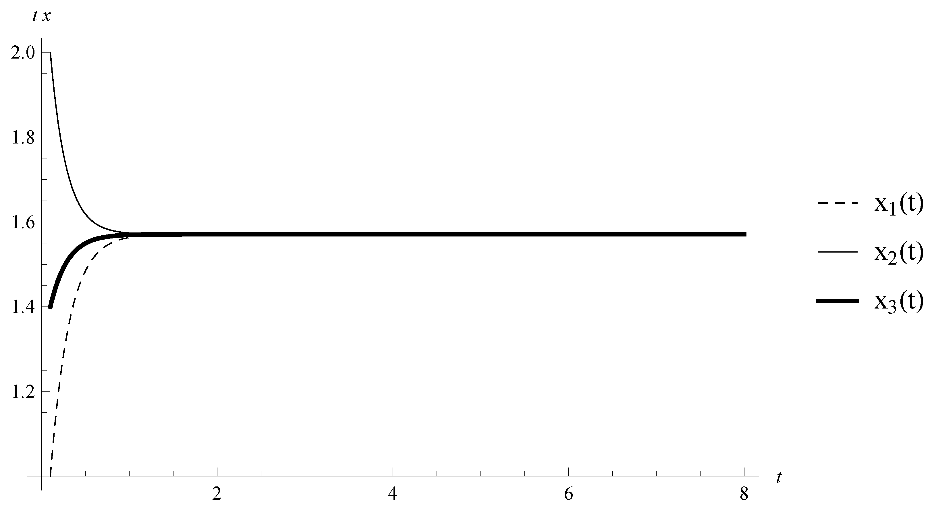
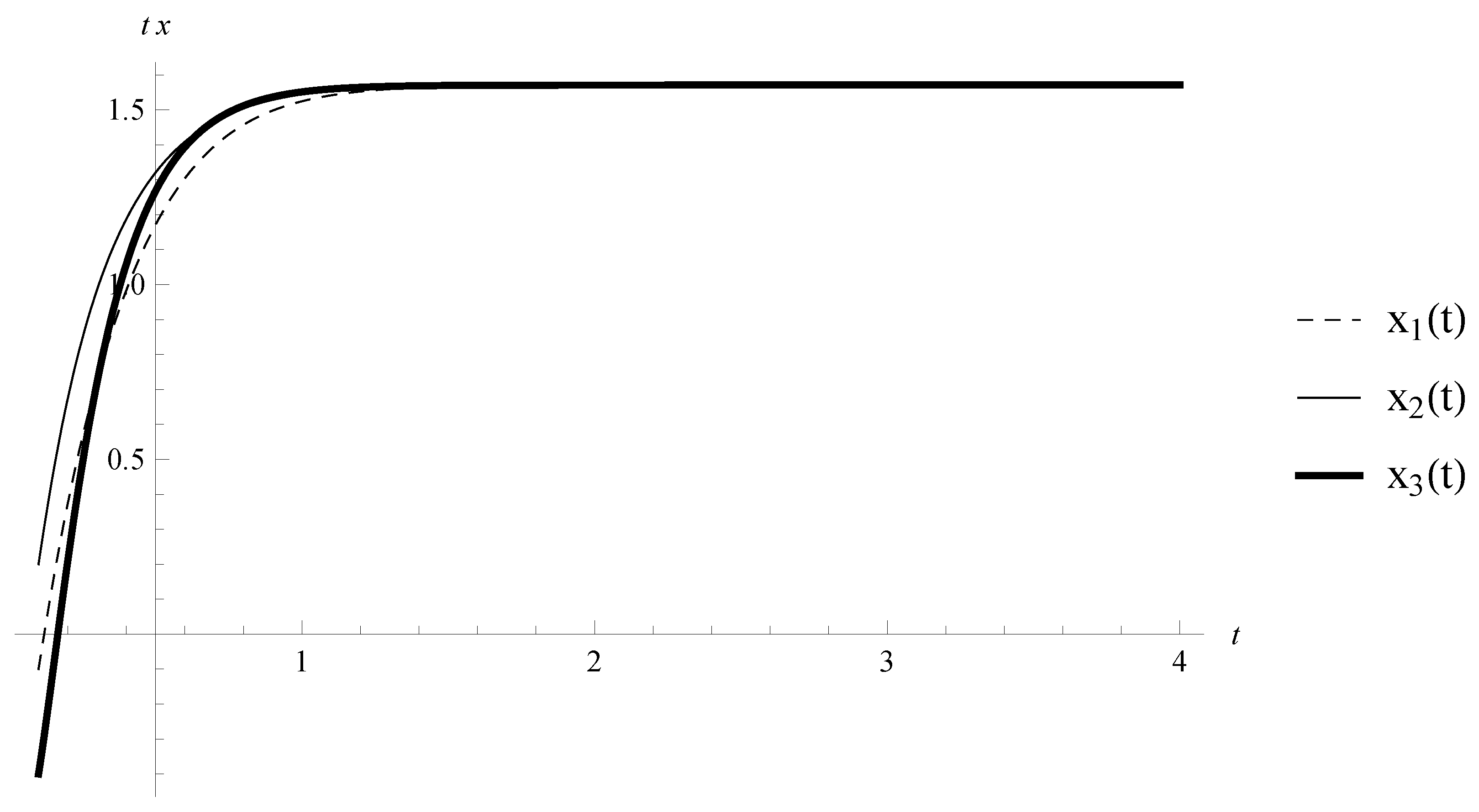
Example 1. Let , and the random variables are exponentially distributed with . Consider the following special case of RINN (2):with , , , and is given by: The point
is the equilibrium point of RINN (
14), i.e., Condition (H4) is satisfied. Now, Assumption (H1) is satisfied with
. In addition, Assumption (H5) is satisfied with
.
Furthermore,
where
is given by:
Therefore, Assumption (H2) is satisfied. Note that Assumption (H3) is satisfied with Lipschitz constants .
Then, the constant
defined by (
12) is
. Next, Assumption (H7) is fulfilled with
because:
Therefore, according to Theorem 1, the equilibrium of RINN (
14) is mean square exponentially stable.
Consider the system (
14) without any kind of impulses. The equilibrium
is asymptotically stable (see
Figure 1 and
Figure 2). Therefore, an appropriate perturbation of the neural networks by impulses at random times can keep the stability properties of the equilibrium.
Remark 10. Note that Condition (H7) is weaker than Condition (3.6) in Theorem 3.2 [16], and as a special case of Theorem 2, we obtain weaker conditions for exponential stability of the Cohen and Grossberg model without any type of impulses. For example, if we consider (14) according to Condition (3.6) [16], the inequality is not satisfied, and Theorem 3.2 [16] does not give us any result about stability (compare with Example 1). Now, consider the following assumption:
(H8) The inequality:
holds.
Theorem 3. Let Assumptions (H1)–(H5), (H7) and (H8) be satisfied. Then, the equilibrium point of RINN (2) is mean exponentially stable. Proof. For any
, we define
. Then:
and:
where
,
.
Then, for
and
according to Remarks 6 and 8, we obtain:
Furthermore, from (H7) and Remark 9, it follows that Condition 2(iii) of Theorem 1 is satisfied. From Theorem 1, we have that Theorem 3 is true. ☐
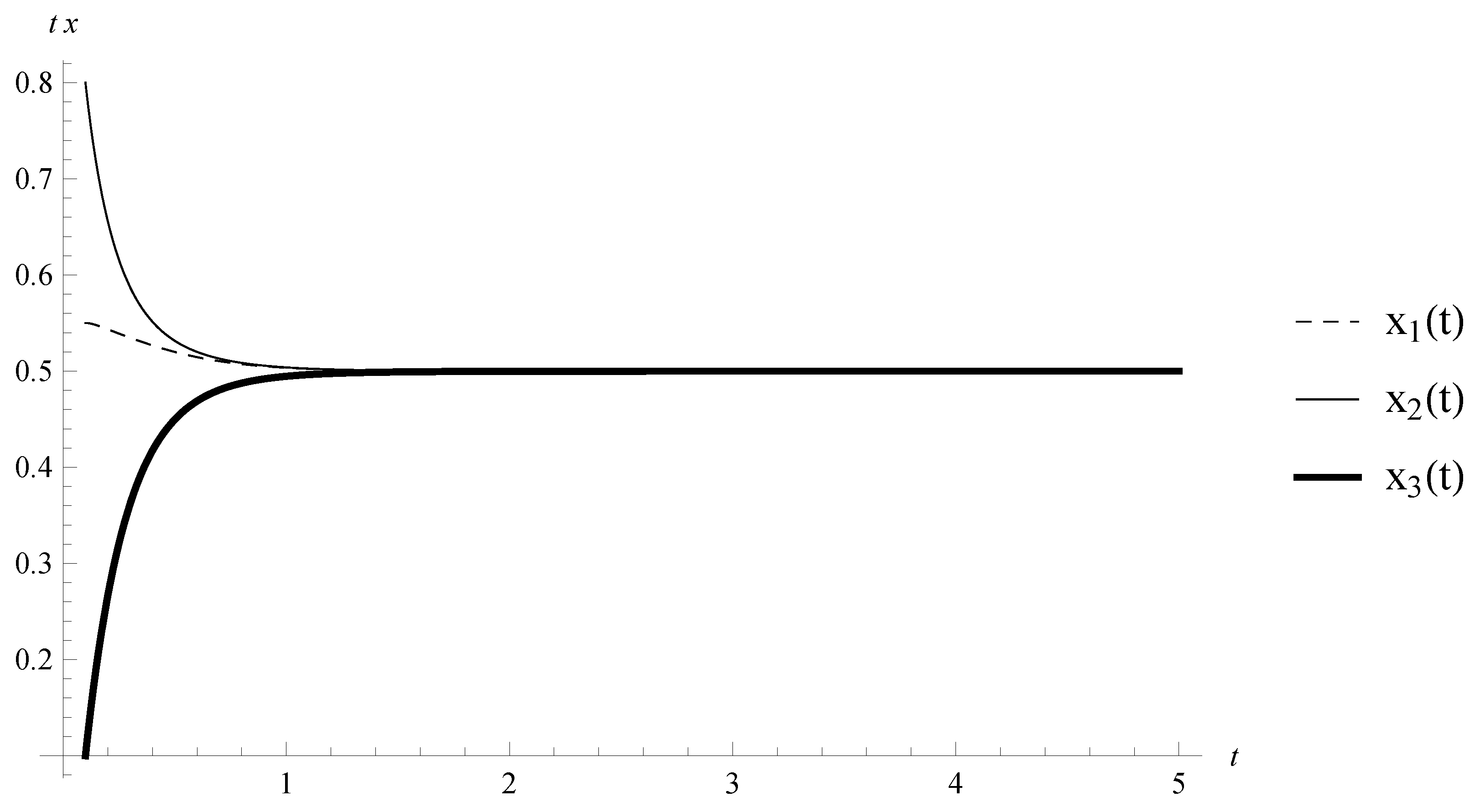
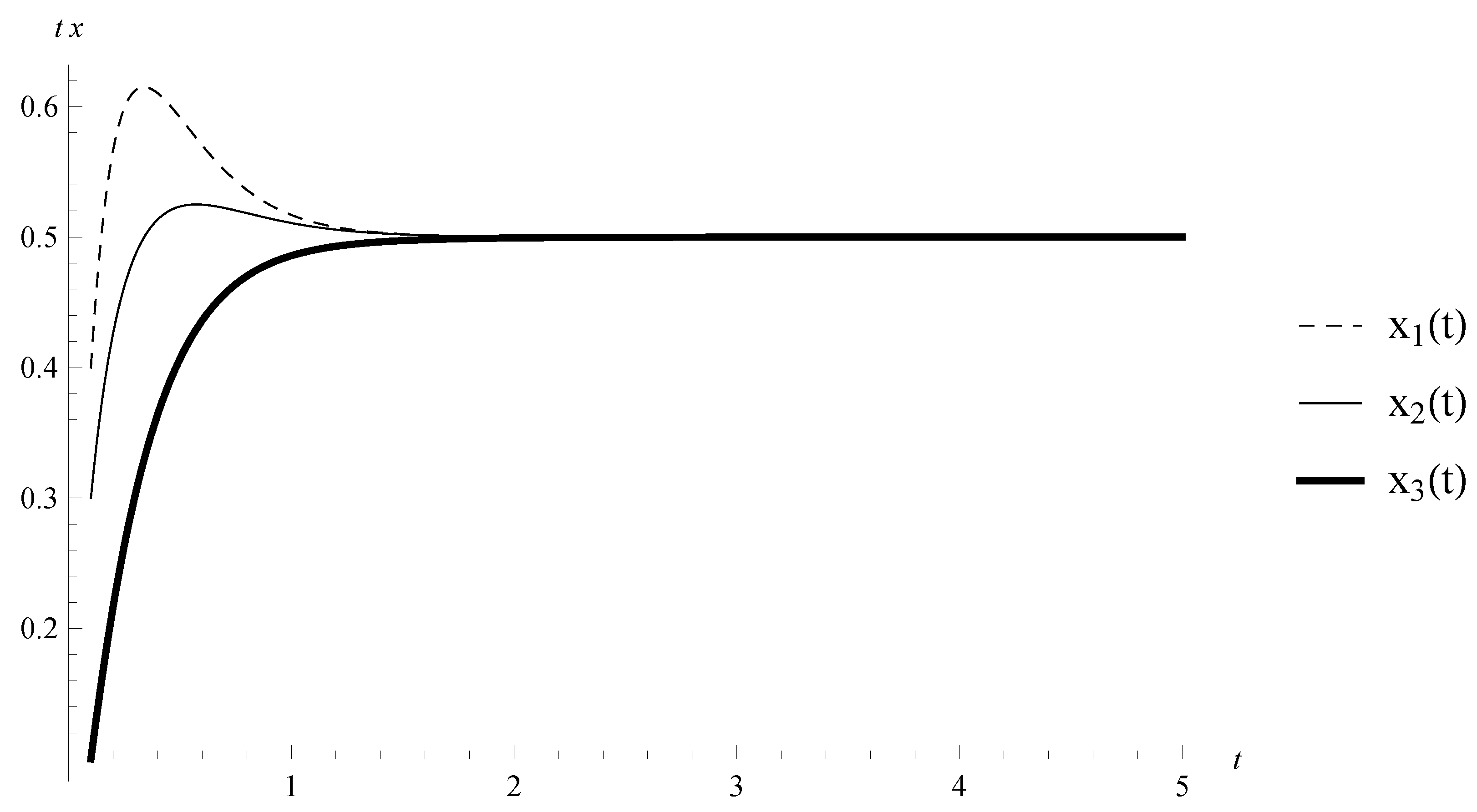
Example 2. Let , , and the random variables are exponentially distributed with . Consider the following special case of RINN (2):with , , , and is given by (15). The point
is the equilibrium point of RINN (
20), i.e., Condition (H4) is satisfied. Now, Assumption (H5) is satisfied with
.
Furthermore,
where
is given by (
16). Therefore, Assumption (H2) is satisfied. Then, the inequality
holds.
According to Theorem 3, the equilibrium of (
20) is mean exponentially stable.
Consider the system (
20) without any kind of impulses. The equilibrium
is asymptotically stable (see
Figure 3 and
Figure 4). Therefore, an appropriate perturbation of the neural networks by impulses at random times can keep the stability properties of the equilibrium.


