The Analytical Solution for the Black-Scholes Equation with Two Assets in the Liouville-Caputo Fractional Derivative Sense

Abstract

It is well known that the Black-Scholes model is used to establish the behavior of the option pricing in the financial market. In this paper, we propose the modified version of Black-Scholes model with two assets based on the Liouville-Caputo fractional derivative. The analytical solution of the proposed model is investigated by the Laplace transform homotopy perturbation method.

1. Introduction

A derivative is one of the financial instruments promising payment at a certain time in the future and the payoff amount depends upon the change of some underlying asset. Its value can be derived from the various sorts of the underlying asset such as shares, bonds, interest rate, commodity, currency, etc. It is unquestioned that options are the primary key of a derivative that is commonly used in the financial market. Hence, the idea of option trading has been continuously developed. The earliest research work was proposed by Corzo et al. [1] using the evidence of the Netherlands having active involvement in trading option. Osborne [2] proposed an option pricing formula using an arithmetic Brownian motion with drift. In the year 1973, Fischer Black and Myron Scholes [3] proposed the Black-Scholes model to investigate the behaviour of the option pricing in a market. Several Mathematical models based on the Black-Scholes equation with five-key components of the strike price, the risk-free rate, the underlying security stock price, the volatility and the mature time have been developed [4,5,6,7].

Several numerical and analytical methods have been studied and developed for finding the solution of Black-Scholes model, for instance, the finite different method [8,9,10,11], finite element method [12] for numerical solutions, and the Mellin transform method [13] and homotopy perturbation method [14,15], Laplace homotopy perturbation method [16] for analytical solutions. Moreover, one of the methods to solve the Black-Scholes equations is radial basis function partition of unity method (RBF-PUM) [17,18] which widely uses to approximate the partial differential equation problem. This method is composed of two methods these are partition of unity (PU) method and radial basis function (RBF) approximants [19,20]. RBF-PUM provides extremely accurate results when applied to data with non-homogeneous density [19].

In general, the Black-Scholes model with 2 assets for option pricing can be written as follows:

$$\begin{array}{c}\hfill \frac{\partial C}{\partial \tau }+\frac{1}{2}\sum _{i=1}^2\sum _{j=1}^2{\sigma }_i{\sigma }_j{\rho }_{ij}{S}_i{S}_j\frac{{\partial }^{2}C}{\partial S_i\partial S_j}+\sum _{i=1}^2(r-q_i)S_i\frac{\partial C}{\partial S_i}-rC=0,\\ \hfill S_1,S_2\in [0,\infty ),\tau \in [0,T]\end{array}$$

with the terminal condition:

$${\displaystyle C(S_1,S_2,T)=\max (\sum _{i=1}^2{\beta }_i{S}_i-K,0),}$$

where $K=max\{K_1,K_2\}$, and the boundary conditions:

$$\begin{array}{c}C(S_1,S_2,\tau )=0\mathrm{as}(S_1,S_2)\to (0,0)\hfill \\ C(S_1,S_2,\tau )=\sum _{i=1}^2{\beta }_i{S}_i-K{e}^{-r(T-\tau )}\mathrm{as}{S}_1\to \infty \mathrm{or}{S}_2\to \infty \hfill \end{array}$$

where:

• C is the call option depending on the underlying stock prices $\{S_1,S_2\}$ at time $\tau$,
• $q_i$ is the dividend yield on the ith underlying stock,
• ${\rho }_{ij}$ is the correlation between the ith and jth underlying stock prices,
• T is the expiration date,
• r is the risk-free interest rate to expiration,
• ${\sigma }_i$ is the volatility of the ith underlying stock,
• $K_i$ is the strike price of the ith underlying stock,
• ${\beta }_i$ is a coefficient so that all risky asset prices are at the same level.

It is noted that the most existing models use the strict assumptions, for example, perfect markets, constant values of both risk-free rate and volatility, log-normal distribution of share price dynamics, no dividends, continuous delta hedging. A divisible number of shares has not adequately represented the reality of the market [21,22,23].

More than three hundred years ago, the fractional differential equation was introduced. Nowadays, fractional calculus could be better for explaining the complicated incidents in the real situation than the traditional calculus. Fractional order models have been used to describe in many areas such as sciences, finance, physics and engineering disciplines [11,12,24,25]. Fractional calculus of the financial market was applied to the Black-Scholes model for expanding the theory of finance.

The time-fractional derivative which is considered in this paper is the Liouville-Caputo derivative because the initial condition for the fractional derivative is similar to the traditional derivative [25].

The Liouville-Caputo-type fractional derivative of order $\alpha$ is defined as [25]:

$$D_{\tau }^{\alpha }C(\tau )=\left\{\begin{array}{cc}{\displaystyle \frac{1}{\mathsf{\Gamma }(1-\alpha )}{\int }_0^{\tau }\frac{C^{\prime }(\xi )}{{(\tau -\xi )}^{\alpha }}d\xi ,}\hfill & 0<\alpha <1,\hfill \\ {\displaystyle \frac{dC}{d\tau },}\hfill & \alpha =1,\hfill \end{array}\right.$$

where $\mathsf{\Gamma }(·)$ is a gamma function.

There are many researches that studied the fractional Black-Scholes model with one asset [11,26,27,28,29,30,31]. The fractional Black-Scholes model is the generalized version of the classical model which extend the limitation of the model. Meng et al. [26] studied the fractional option pricing using Black-Scholes model. They applied the fractional Black-Scholes model to call option price for bank foreign exchange in China. Their results show that the fractional Black-Scholes model is better than the classical Black-Sholes model for estimating the effect in the market mechanism [26].

In this paper, we use the application of the Laplace transform Homotopy Perturbation Method (LHPM) to obtain the explicit solution of the time fractional Black-Scholes model. The LHPM is a method that combines with Homotopy Perturbation Method and Laplace transform. The LHPM gives an explicit solution which is a convergent series. We focus on the time fractional Black-Scholes model with two assets for the European call option. The LHPM is utilized for solving the problem. The analytical solution is a valuable tool to study the behaviors of the solution which are difficult to get the numerical solution especially fractional partial differential equations. The analytical solution provides a useful tool for studying financial behavior.

The paper is organized as follows. We present the time fractional Black-Scholes model in Section 2. The fractional derivatives are described in the sense of the Liouville-Caputo fractional derivative. The LHPM is presented in Section 3. In Section 3.1, the explicit solution of this problem is carried out by using LHPM. In addition, numerical examples and discussions are obtained in Section 4. Finally, a conclusion is presented in Section 5.

2. Mathematical Model

We consider the standard Black-Scholes partial differential equation with two assets for European-style option, efficient markets, perfect liquidity and no dividends during the option’s life. Throughout this paper, we assume that ${\sigma }_1,{\sigma }_2,\rho$ and r are constants.

$$\begin{array}{cc}\hfill \frac{\partial c}{\partial \tau }& +\frac{1}{2}{\sigma }_1^2{S}_1^2\frac{{\partial }^{2}c}{\partial S_1^2}+\frac{1}{2}{\sigma }_2^2{S}_2^2\frac{{\partial }^{2}c}{\partial S_2^2}+\rho {\sigma }_1{\sigma }_2{S}_1{S}_2\frac{\partial c^2}{\partial S_1\partial S_2}\hfill \\ \hfill & +r\left[S_1\frac{\partial c}{\partial S_1}+S_2\frac{\partial c}{\partial S_2}\right]-rc=0,\mathrm{for}{S}_1,S_2\in [0,\infty ),\tau \in [0,T]\hfill \end{array}$$

(1)

with the terminal condition:

$$c(S_1,S_2,T)=max\left\{{\beta }_1{S}_1+{\beta }_2{S}_2-K,0\right\},$$

and boundary conditions:

$$\begin{array}{c}c(S_1,S_2,\tau )=0\mathrm{as}(S_1,S_2)\to 0\mathrm{and}\hfill \\ c(S_1,S_2,\tau )={\beta }_1{S}_1+{\beta }_2{S}_2-K{e}^{-r(T-\tau )}\mathrm{as}{S}_1\to \infty \mathrm{or}{S}_2\to \infty .\hfill \end{array}$$

By changing the variables [32]:

$$\begin{array}{c}x=ln(S_1)-\left(r-\frac{1}{2}{\sigma }_1^2\right)\tau \mathrm{and}y=ln(S_2)-\left(r-\frac{1}{2}{\sigma }_2^2\right)\tau ,\hfill \end{array}$$

Equation (1) can be written as:

$$\begin{array}{c}\hfill \frac{\partial c}{\partial \tau }+\frac{1}{2}{\sigma }_1^2\frac{{\partial }^{2}c}{\partial x^2}+\frac{1}{2}{\sigma }_2^2\frac{{\partial }^{2}c}{\partial y^2}+\rho {\sigma }_1{\sigma }_2\frac{{\partial }^{2}c}{\partial x\partial y}-rc=0,(x,y,\tau )\in \mathbb{R}\times \mathbb{R}\times [0,T]\end{array}$$

(2)

which satisfies the terminal condition:

$$c(x,y,T)=max\left({\beta }_1{e}^{x+(r-\frac{1}{2}{\sigma }_1^2)T}+{\beta }_2{e}^{y+(r-\frac{1}{2}{\sigma }_2^2)T}-K,0\right),$$

and boundary conditions:

$$\begin{array}{c}c(x,y,\tau )=0,\mathrm{as}(x,y)\to -\infty \mathrm{and}\hfill \\ c(x,y,\tau )={\beta }_1{e}^{x+(r-\frac{1}{2}{\sigma }_1^2)\tau }+{\beta }_2{e}^{y+(r-\frac{1}{2}{\sigma }_2^2)\tau }-K{e}^{-r(T-\tau )},\hfill \\ \mathrm{as}x\to \infty \mathrm{or}y\to \infty .\hfill \end{array}$$

By changing again of variables for eliminating the last term on the left hand side of Equation (2), we define v as:

$$c(x,y,\tau )=e^{-r(T-\tau )}v(x,y,\tau ),$$

and substitute into Equation (2), we have

$$\begin{array}{c}\hfill \frac{\partial v}{\partial \tau }+\frac{1}{2}{\sigma }_1^2\frac{{\partial }^{2}v}{\partial x^2}+\frac{1}{2}{\sigma }_2^2\frac{{\partial }^{2}v}{\partial y^2}+\rho {\sigma }_1{\sigma }_2\frac{{\partial }^{2}v}{\partial x\partial y}=0,(x,y,\tau )\in \mathbb{R}\times \mathbb{R}\times [0,T]\end{array}$$

(3)

with the terminal condition:

$$v(x,y,T)=max\left({\beta }_1{e}^{x+(r-\frac{1}{2}{\sigma }_1^2)T}+{\beta }_2{e}^{y+(r-\frac{1}{2}{\sigma }_2^2)T}-K,0\right),$$

(4)

and the boundary conditions:

$$\begin{array}{c}v(x,y,\tau )=0,\mathrm{as}(x,y)\to -\infty \mathrm{and}\hfill \\ v(x,y,\tau )={\beta }_1{e}^{x+rT-\frac{1}{2}{\sigma }_1^2\tau }+{\beta }_2{e}^{y+rT-\frac{1}{2}{\sigma }_2^2\tau }-K,\mathrm{as}x\to \infty \mathrm{or}y\to \infty .\hfill \end{array}$$

(5)

To be able to solve the initial boundary value problem (3)–(5), a forward time coordinate

$$t=T-\tau$$

is introduced and used in Equation (3). Hence, we obtain

$$\begin{array}{c}\hfill \frac{\partial v}{\partial t}=\frac{1}{2}{\sigma }_1^2\frac{{\partial }^{2}v}{\partial x^2}+\frac{1}{2}{\sigma }_2^2\frac{{\partial }^{2}v}{\partial y^2}+\rho {\sigma }_1{\sigma }_2\frac{{\partial }^{2}v}{\partial x\partial y},(x,y,\tau )\in \mathbb{R}\times \mathbb{R}\times [0,T],\end{array}$$

subject to the initial condition:

$$v(x,y,0)=max\left(\widetilde{{\beta }_1}{e}^x+\widetilde{{\beta }_2}{e}^y-K,0\right),$$

(6)

and the boundary conditions:

$$\begin{array}{c}v(x,y,t)=0,\mathrm{as}(x,y)\to -\infty \mathrm{and}\hfill \\ v(x,y,t)=\widetilde{{\beta }_1}{e}^{x+\frac{1}{2}{\sigma }_1^{2}t}+\widetilde{{\beta }_2}{e}^{y+\frac{1}{2}{\sigma }_2^{2}t}-K,\mathrm{as}x\to \infty \mathrm{or}y\to \infty .\hfill \end{array}$$

where $\widetilde{{\beta }_1}={\beta }_1{e}^{(r-\frac{1}{2}{\sigma }_1^2)T}$ and $\widetilde{{\beta }_2}={\beta }_2{e}^{(r-\frac{1}{2}{\sigma }_2^2)T}$.

By replacing the Liouville Caputo fractional derivative, we obtain the following fractional-time order Black-Scholes model with $\alpha \in (0,1]$ equipped with the initial and boundary conditions:

$$\begin{array}{c}\hfill D_t^{\alpha }v=\frac{1}{2}{\sigma }_1^2\frac{{\partial }^{2}v}{\partial x^2}+\frac{1}{2}{\sigma }_2^2\frac{{\partial }^{2}v}{\partial y^2}+\rho {\sigma }_1{\sigma }_2\frac{{\partial }^{2}v}{\partial x\partial y},(x,y,\tau )\in \mathbb{R}\times \mathbb{R}\times [0,T],\end{array}$$

(7)

subject to the initial condition:

$$v(x,y,0)=max\left(\widetilde{{\beta }_1}{e}^x+\widetilde{{\beta }_2}{e}^y-K,0\right),$$

(8)

and boundary conditions:

$$\begin{array}{c}v(x,y,t)=0,\mathrm{as}(x,y)\to -\infty \mathrm{and}\hfill \\ v(x,y,t)=\widetilde{{\beta }_1}{e}^{x+\frac{1}{2}{\sigma }_1^{2}t}+\widetilde{{\beta }_2}{e}^{y+\frac{1}{2}{\sigma }_2^{2}t}-K,\mathrm{as}x\to \infty \mathrm{or}y\to \infty .\hfill \end{array}$$

(9)

where $\widetilde{{\beta }_1}={\beta }_1{e}^{(r-\frac{1}{2}{\sigma }_1^2)T}$ and $\widetilde{{\beta }_2}={\beta }_2{e}^{(r-\frac{1}{2}{\sigma }_2^2)T}$.

3. Basic Ideas of Time Fractional Black-Scholes Model with LHPM

In this section, the general form of the time-dependent differential equation can be expressed in the form of:

$$A(u(x,y,t))-f(x,y,t)=0,$$

(10)

where $u(x,y,t)$ denotes an unknown function, $f(x,y,t)$ denotes a known analytic function and A is determined by:

$$\begin{array}{c}\hfill A(u(x,y,t))=D_t^{\alpha }u(x,y,t)+\tilde{N}(u(x,y,t))\mathrm{for}(x,y,t)\in \mathbb{R}\times \mathbb{R}\times [0,T].\end{array}$$

A general equation can be rewritten as:

$$\begin{array}{c}\hfill D_t^{\alpha }u(x,y,t)+\tilde{N}(u(x,y,t))=f(x,y,t),(x,y,t)\in \mathbb{R}\times \mathbb{R}\times [0,T],\end{array}$$

(11)

with the initial condition:

$$u(x,y,0)=h(x,y)\mathrm{for}\mathrm{any}(x,y)\in \mathbb{R}\times \mathbb{R}$$

and the boundary condition:

$$B\left(u,\frac{\partial u}{\partial x},\frac{\partial u}{\partial y},\frac{\partial u}{\partial t}\right)=0,$$

where B is a boundary operator.

Firstly, in Equation (11), taking the Laplace transform with respect to time variable t yields

$$\mathcal{L}\left\{D_t^{\alpha }u(x,y,t)\right\}+\mathcal{L}\left\{\tilde{N}(u(x,y,t))\right\}=\mathcal{L}\left\{f(x,y,t)\right\}.$$

Using the Laplace transform of Liouville-Caputo fractional derivative [33], we then obtain

$$\begin{array}{cc}\hfill \mathcal{L}\left\{u(x,y,t)\right\}=& s^{-\alpha }h(x,y)-s^{-\alpha }\mathcal{L}\left\{\tilde{N}(u(x,y,t))\right\}+s^{-\alpha }\mathcal{L}\left\{f(x,y,t)\right\}.\hfill \end{array}$$

(12)

By taking the inverse Laplace transform on Equation (12), we have

$$u(x,y,t)=G(x,y,t)-{\mathcal{L}}^{-1}\left\{s^{-\alpha }\mathcal{L}\left\{\tilde{N}(u(x,y,t))\right\}\right\},$$

where the function $G(x,y,t)$ presents the term arising from the source term and the prescribed initial conditions and boundary conditions.

We now using the technique of HPM [14,15] to construct the function $\nu (x,y,t;p)$. We set

$$\begin{array}{cc}\hfill H(\nu (x,y,t;p),p)=& (1-p)[\nu (x,y,t;p)-\widetilde{{\nu }_0}(x,y,t)]\hfill \\ \hfill & +p[\nu (x,y,t;p)-G(x,y,t)\hfill \\ \hfill & +{\mathcal{L}}^{-1}\left\{s^{-\alpha }\mathcal{L}\left\{\tilde{N}(\nu (x,y,t;p))\right\}\right\}]=0,\hfill \end{array}$$

(13)

where $p\in [0,1]$ denotes homotopy parameter or an embedding parameter and $\widetilde{{\nu }_0}(x,y,t)$ denotes the initial approximation of Equation (13). Rearranging (13) gives

$$\begin{array}{cc}\hfill \nu (x,y,t;p)=& \widetilde{{\nu }_0}(x,y,t)-p[\widetilde{{\nu }_0}(x,y,t)-G(x,y,t)\hfill \\ \hfill & +{\mathcal{L}}^{-1}\left\{s^{-\alpha }\mathcal{L}\left\{\tilde{N}(\nu (x,y,t;p))\right\}\right\}].\hfill \end{array}$$

(14)

For $p=0$ and $p=1$, we have

$$\begin{array}{cc}\hfill H(\nu (x,y,t;0),0)=& \nu (x,y,t;0)-\widetilde{{\nu }_0}(x,y,t)=0,\hfill \\ \hfill H(\nu (x,y,t;1),1)=& \nu (x,y,t;1)-G(x,y,t)\hfill \\ \hfill & +{\mathcal{L}}^{-1}\left\{s^{-\alpha }\mathcal{L}\left\{\tilde{N}(\nu (x,y,t;1))\right\}\right\}=0.\hfill \end{array}$$

Let

$$\nu (x,y,t;p)=\sum _{n=0}^{\infty }{p}^n{\nu }_n(x,y,t).$$

(15)

From Equations (14) and (15), we have

$$\begin{array}{cc}\hfill \sum _{n=0}^{\infty }{p}^n{\nu }_n(x,y,t)& =\widetilde{{\nu }_0}(x,y,t)-p[\widetilde{{\nu }_0}(x,y,t)-G(x,y,t)\hfill \\ \hfill & +{\mathcal{L}}^{-1}\left\{s^{-\alpha }\mathcal{L}\left\{\tilde{N}(\sum _{n=0}^{\infty }{p}^n{\nu }_n(x,y,t))\right\}\right\}].\hfill \end{array}$$

(16)

By equating the coefficients corresponding to the power of p on both sides of Equation (16), the sequence ${\nu }_n$ is carried out as follows:

$$\begin{array}{cc}\hfill {\nu }_0(x,y,t)=& \widetilde{{\nu }_0}(x,y,t),\hfill \\ \hfill {\nu }_1(x,y,t)=& G(x,y,t)-\widetilde{{\nu }_0}(x,y,t)-{\mathcal{L}}^{-1}\left\{s^{-\alpha }\mathcal{L}\left\{\tilde{N}(\widetilde{{\nu }_0}(x,y,t))\right\}\right\},\hfill \\ \hfill {\nu }_m(x,y,t)=& -{\mathcal{L}}^{-1}\left\{s^{-\alpha }\mathcal{L}\left\{\tilde{N}({\nu }_{m-1}(x,y,t))\right\}\right\}\mathrm{when}m\ge 2.\hfill \end{array}$$

(17)

When p converges to 1, the approximate solution of Equation (10) can be expressed in the form of:

$$u(x,y,t)=\sum _{n=0}^{\infty }{\nu }_n(x,y,t),$$

(18)

which leads to the explicit solution when infinite series converges.

3.1. A Solution of Time Fractional Black-Scholes Model by LHPM

In this section, we find the solution of time fractional Black-Scholes model (7) subjecting to the terminal Condition (8) and boundary Condition (9) by LHPM techniques.

Firstly, we let

$$\tilde{N}(v(x,y,t))=\frac{1}{2}{\sigma }_1^2\frac{{\partial }^{2}v}{\partial x^2}+\frac{1}{2}{\sigma }_2^2\frac{{\partial }^{2}v}{\partial y^2}+\rho {\sigma }_1{\sigma }_2\frac{{\partial }^{2}v}{\partial x\partial y},$$

and express Equation (7) in the general form of:

$$D_t^{\alpha }v(x,y,t)=\tilde{N}(v(x,y,t)).$$

By taking the Laplace transform with respect to time variable t, we get

$$\mathcal{L}\left\{D_t^{\alpha }v(x,y,t)\right\}=\mathcal{L}\left\{\tilde{N}(v(x,y,t))\right\}.$$

(19)

It follows from Laplace transform of the Liouville-Caputo fractional derivative that Equation (19) becomes,

$$\begin{array}{cc}\hfill \mathcal{L}\left\{v(x,y,t)\right\}=& \frac{1}{s^{}}\max (\widetilde{{\beta }_1}{e}^x+\widetilde{{\beta }_2}{e}^y-K,0)+\frac{1}{s^{\alpha }}\mathcal{L}\{\frac{1}{2}{\sigma }_1^2\frac{{\partial }^{2}v}{\partial x^2}+\frac{1}{2}{\sigma }_2^2\frac{{\partial }^{2}v}{\partial y^2}\hfill \\ \hfill & +\rho {\sigma }_1{\sigma }_2\frac{{\partial }^{2}v}{\partial x\partial y}\}.\hfill \end{array}$$

(20)

The inverse Laplace transform of an Equation (20) is obtained as:

$$\begin{array}{cc}\hfill v(x,y,t)=& \max (\widetilde{{\beta }_1}{e}^x+\widetilde{{\beta }_2}{e}^y-K,0)+{\mathcal{L}}^{-1}\left\{\frac{1}{s^{\alpha }}\mathcal{L}\right\{\frac{1}{2}{\sigma }_1^2\frac{{\partial }^{2}v}{\partial x^2}+\frac{1}{2}{\sigma }_2^2\frac{{\partial }^{2}v}{\partial y^2}\hfill \\ \hfill & +\rho {\sigma }_1{\sigma }_2\frac{{\partial }^{2}v}{\partial x\partial y}\left\}\right\}.\hfill \end{array}$$

By applying techniques of HPM, we can construct the function

$$v(x,y,t;p):\mathbb{R}\times \mathbb{R}\times [0,T]\times [0,1]\to \mathbb{R}$$

which satisfies the following equation

$$\begin{array}{c}(1-p)(v(x,y,t;p)-\widetilde{v_0}(x,y,t))+p[v(x,y,t;p)-\max (\widetilde{{\beta }_1}{e}^x+\widetilde{{\beta }_2}{e}^y-K,0)\hfill \\ -{\mathcal{L}}^{-1}\left\{\frac{1}{s^{\alpha }}\mathcal{L}\left\{\frac{1}{2}{\sigma }_1^2\frac{{\partial }^{2}v}{\partial x^2}+\frac{1}{2}{\sigma }_2^2\frac{{\partial }^{2}v}{\partial y^2}+\rho {\sigma }_1{\sigma }_2\frac{{\partial }^{2}v}{\partial x\partial y}\right\}\right\}]=0\hfill \end{array}$$

or

$$\begin{array}{cc}\hfill v(x,y,t;p)=& \widetilde{v_0}(x,y,t)-p\widetilde{v_0}(x,y,t)+pmax(\widetilde{{\beta }_1}{e}^x+\widetilde{{\beta }_2}{e}^y-K,0)\hfill \\ \hfill & +p{\mathcal{L}}^{-1}\left\{\frac{1}{s^{\alpha }}\mathcal{L}\left\{\frac{1}{2}{\sigma }_1^2\frac{{\partial }^{2}v}{\partial x^2}+\frac{1}{2}{\sigma }_2^2\frac{{\partial }^{2}v}{\partial y^2}+\rho {\sigma }_1{\sigma }_2\frac{{\partial }^{2}v}{\partial x\partial y}\right\}\right\},\hfill \end{array}$$

(21)

where $p\in [0,1]$ is an embedded parameter and $\widetilde{v_0}(x,y,t)$ is an initial approximation of Equation (21) which can be freely chosen [34].

For this model, we choose $\widetilde{v_0}(x,y,t)$ as:

$$\widetilde{v_0}(x,y,t)=\max (\widetilde{{\beta }_1}{e}^x+\widetilde{{\beta }_2}{e}^y-K,0)+e^{x+y}{t}^{\alpha }.$$

Next we substitute $\widetilde{v_0}(x,y,t)$ in Equation (21) to obtain

$$\begin{array}{cc}\hfill v(x,y,t;p)=& \max (\widetilde{{\beta }_1}{e}^x+\widetilde{{\beta }_2}{e}^y-K,0)+e^{x+y}{t}^{\alpha }+p(-e^{x+y}{t}^{\alpha }\hfill \\ \hfill & +{\mathcal{L}}^{-1}\left\{\frac{1}{s^{\alpha }}\mathcal{L}\left\{\frac{1}{2}{\sigma }_1^2\frac{{\partial }^{2}v}{\partial x^2}+\frac{1}{2}{\sigma }_2^2\frac{{\partial }^{2}v}{\partial y^2}+\rho {\sigma }_1{\sigma }_2\frac{{\partial }^{2}v}{\partial x\partial y}\right\}\right\}).\hfill \end{array}$$

(22)

For homotopy perturbation method, the solution of Equation (7) can be assumed that

$$\begin{array}{c}\hfill v(x,y,t;p)=\sum _{i=0}^{\infty }{p}^n{\varphi }_n(x,y,t).\end{array}$$

(23)

By substituting Equation (23) into Equation (22), we obtain

$$\begin{array}{cc}\hfill \sum _{n=0}^{\infty }{p}^n{\varphi }_n(x,y,t)=& max(\widetilde{{\beta }_1}{e}^x+\widetilde{{\beta }_2}{e}^y-K,0)+e^{x+y}{t}^{\alpha }+p\left(-e^{x+y}{t}^{\alpha }\right.\hfill \\ \hfill & +{\mathcal{L}}^{-1}\left\{\frac{1}{s^{\alpha }}\mathcal{L}\right\{\frac{1}{2}{\sigma }_1^2\sum _{n=0}^{\infty }{p}^n\frac{{\partial }^2{\varphi }_n}{\partial x^2}\hfill \\ \hfill & +\frac{1}{2}{\sigma }_2^2\sum _{n=0}^{\infty }{p}^n\frac{{\partial }^2{\varphi }_n}{\partial y^2}\left.+\rho {\sigma }_1{\sigma }_2\sum _{n=0}^{\infty }{p}^n\frac{{\partial }^2{\varphi }_n}{\partial x\partial y}\left\}\right\}\right).\hfill \end{array}$$

(24)

By equating the corresponding power of p on both sides of Equation (24), we have

$$\begin{array}{cc}\hfill {\varphi }_0(x,y,t)=& max(\widetilde{{\beta }_1}{e}^x+\widetilde{{\beta }_2}{e}^y-K,0)+e^{x+y}{t}^{\alpha }\hfill \\ \hfill {\varphi }_1(x,y,t)=& -e^{x+y}{t}^{\alpha }+{\mathcal{L}}^{-1}\left\{\frac{1}{s^{\alpha }}\mathcal{L}\left\{\frac{1}{2}{\sigma }_1^2\frac{{\partial }^2{\varphi }_0}{\partial x^2}+\frac{1}{2}{\sigma }_2^2\frac{{\partial }^2{\varphi }_0}{\partial y^2}+\rho {\sigma }_1{\sigma }_2\frac{{\partial }^2{\varphi }_0}{\partial x\partial y}\right\}\right\}\hfill \\ \hfill {\varphi }_i(x,y,t)=& -e^{x+y}{t}^{\alpha }+{\mathcal{L}}^{-1}\left\{\frac{1}{s^{\alpha }}\mathcal{L}\right\{\frac{1}{2}{\sigma }_1^2\frac{{\partial }^2{\varphi }_{i-1}}{\partial x^2}+\frac{1}{2}{\sigma }_2^2\frac{{\partial }^2{\varphi }_{i-1}}{\partial y^2}\hfill \\ \hfill & +\rho {\sigma }_1{\sigma }_2\frac{{\partial }^2{\varphi }_{i-1}}{\partial x\partial y}\left\}\right\},\mathrm{for}i\ge 2.\hfill \end{array}$$

Then, we can write ${\varphi }_0,{\varphi }_1,{\varphi }_2,{\varphi }_3,\dots$ in the general form, i.e.,

$$\begin{array}{cc}\hfill {\varphi }_0(x,y,t)=& max(\widetilde{{\beta }_1}{e}^x+\widetilde{{\beta }_2}{e}^y-K,0)+e^{x+y}{t}^{\alpha }\hfill \\ \hfill {\varphi }_n(x,y,t)=& \frac{t^{n\alpha }}{\mathsf{\Gamma }(n\alpha +1)}\left(\frac{1}{2^n}{\sigma }_1^{2n}\max (\widetilde{{\beta }_1}{e}^x,0)+\frac{1}{2^n}{\sigma }_2^{2n}\max (\widetilde{{\beta }_2}{e}^y,0)\right)\hfill \\ \hfill & +e^{x+y}\frac{t^{(n+1)\alpha }\mathsf{\Gamma }(\alpha +1)}{\mathsf{\Gamma }((n+1)\alpha +1)}{\left(\frac{{\sigma }_1^2}{2}+\frac{{\sigma }_2^2}{2}+\rho {\sigma }_1{\sigma }_2\right)}^n\hfill \\ \hfill & -e^{x+y}\frac{t^{n\alpha }\mathsf{\Gamma }(\alpha +1)}{\mathsf{\Gamma }(n\alpha +1)}{\left(\frac{{\sigma }_1^2}{2}+\frac{{\sigma }_2^2}{2}+\rho {\sigma }_1{\sigma }_2\right)}^{(n-1)}\mathrm{when}n\ge 1.\hfill \end{array}$$

From (23), the solution $v(x,y,t)$ of the Equation (7) can be written by:

$$\begin{array}{cc}\hfill v(x,& y,t;p)=max(\widetilde{{\beta }_1}{e}^x+\widetilde{{\beta }_2}{e}^y-K,0)+e^{x+y}{t}^{\alpha }\hfill \\ \hfill & +\sum _{n=0}^{\infty }{p}^{n+1}\left\{\frac{t^{(n+1)\alpha }}{\mathsf{\Gamma }((n+1)\alpha +1)}\right(\frac{1}{2^{(n+1)}}{\sigma }_1^{2(n+1)}\max (\widetilde{{\beta }_1}{e}^x,0)\hfill \\ \hfill & +\frac{1}{2^{(n+1)}}{\sigma }_2^{2(n+1)}\max (\widetilde{{\beta }_2}{e}^y,0))\hfill \\ \hfill & +e^{x+y}\frac{t^{(n+2)\alpha }\mathsf{\Gamma }(\alpha +1)}{\mathsf{\Gamma }((n+2)\alpha +1)}{\left(\frac{{\sigma }_1^2}{2}+\frac{{\sigma }_2^2}{2}+\rho {\sigma }_1{\sigma }_2\right)}^{(n+1)}\hfill \\ \hfill & -e^{x+y}\frac{t^{(n+1)\alpha }\mathsf{\Gamma }(\alpha +1)}{\mathsf{\Gamma }((n+1)\alpha +1)}{\left(\frac{{\sigma }_1^2}{2}+\frac{{\sigma }_2^2}{2}+\rho {\sigma }_1{\sigma }_2\right)}^n\}.\hfill \end{array}$$

By setting p converges to 1, we get

$$\begin{array}{cc}\hfill v(x,& y,t;1)=max(\widetilde{{\beta }_1}{e}^x+\widetilde{{\beta }_2}{e}^y-K,0)+e^{x+y}{t}^{\alpha }+\sum _{n=0}^{\infty }\{\frac{t^{(n+1)\alpha }}{\mathsf{\Gamma }((n+1)\alpha +1)}\hfill \\ \hfill & \times \left(\frac{1}{2^{(n+1)}}{\sigma }_1^{2(n+1)}\max (\widetilde{{\beta }_1}{e}^x,0)+\frac{1}{2^{(n+1)}}{\sigma }_2^{2(n+1)}\max (\widetilde{{\beta }_2}{e}^y,0)\right)\hfill \\ \hfill & +e^{x+y}\frac{t^{(n+2)\alpha }\mathsf{\Gamma }(\alpha +1)}{\mathsf{\Gamma }((n+2)\alpha +1)}{\left(\frac{{\sigma }_1^2}{2}+\frac{{\sigma }_2^2}{2}+\rho {\sigma }_1{\sigma }_2\right)}^{(n+1)}\hfill \\ \hfill & -e^{x+y}\frac{t^{(n+1)\alpha }\mathsf{\Gamma }(\alpha +1)}{\mathsf{\Gamma }((n+1)\alpha +1)}{\left(\frac{{\sigma }_1^2}{2}+\frac{{\sigma }_2^2}{2}+\rho {\sigma }_1{\sigma }_2\right)}^n\}\hfill \end{array}$$

Therefore, we get the explicit solution of Equation (7):

$$\begin{array}{c}v(x,y,t)=max(\widetilde{{\beta }_1}{e}^x+\widetilde{{\beta }_2}{e}^y-K,0)+e^{x+y}{t}^{\alpha }\hfill \\ +max(\widetilde{{\beta }_1}{e}^x,0)\frac{t^{\alpha }{\sigma }_1^2}{2}{E}_{\alpha ,\alpha +1}(\frac{t^{\alpha }{\sigma }_1^2}{2})+\max (\widetilde{{\beta }_2}{e}^y,0)\frac{t^{\alpha }{\sigma }_2^2}{2}{E}_{\alpha ,\alpha +1}(\frac{t^{\alpha }{\sigma }_2^2}{2})\hfill \\ +\left(e^{x+y}\left(\frac{{\sigma }_1^2}{2}+\frac{{\sigma }_2^2}{2}+\rho {\sigma }_1{\sigma }_2\right)\mathsf{\Gamma }(\alpha +1)t^{2\alpha }{E}_{\alpha ,2\alpha +1}\left(t^{\alpha }\left(\frac{{\sigma }_1^2}{2}+\frac{{\sigma }_2^2}{2}+\rho {\sigma }_1{\sigma }_2\right)\right)\right)\hfill \\ -e^{x+y}\mathsf{\Gamma }(\alpha +1)t^{\alpha }{E}_{\alpha ,\alpha +1}\left(t^{\alpha }\left(\frac{{\sigma }_1^2}{2}+\frac{{\sigma }_2^2}{2}+\rho {\sigma }_1{\sigma }_2\right)\right)\hfill \end{array}$$

(25)

where $E_{a,b}(z)={\sum }_{k=0}^{\infty }\frac{z^k}{\mathsf{\Gamma }(ak+b)}$ is the Generalized Mittag-Leffler function [35] which a and b are constants.

4. Numerical Examples

In this section, an series solution of European call option based on Black-Scholes model with two assets as in Equation (25) is computed by using MATLAB programming. The simulations are carried out using the financial parameters given in Table 1.

Table 1. Parameters of the numerical solution.

Parameters	Value
strike price, K (dollars)	70
risk-free interest rate (per year), r	$5\%$
maturity time, T (year)	1
volatility of the underlying first assets (per year), ${\sigma }_1$	$10\%$
volatility of the underlying second assets (per year), ${\sigma }_2$	$20\%$
correlation, $\rho$	0.5
${\beta }_1$	2
${\beta }_2$	1

The graphs of the transformed explicit solution v and original explicit solution c in the case of call option are plotted in Figure 1, Figure 2, Figure 3, Figure 4 and Figure 5. In Figure 1, the solutions v and c are plotted at a day before an expiration date over a range of $0\le S_1\le 200$ and $0\le S_2\le 200$ surrounding at the strike price with order $\alpha =0.9$. The results show that the option values increase significantly when the stock prices increase.

Figure 1. (a) Transformed explicit solution, v, and (b) call option price, c, for $\alpha =0.9$ at a day before an expiration date.

Figure 2. (a) Transformed explicit solution, v, and (b) call option price, c, for all time of order $\alpha =0.9$ with $S_2=10$.

Figure 3. (a) Transformed explicit solution, v, and (b) call option price, c, for all time of order $\alpha =0.9$ with $S_1=10$.

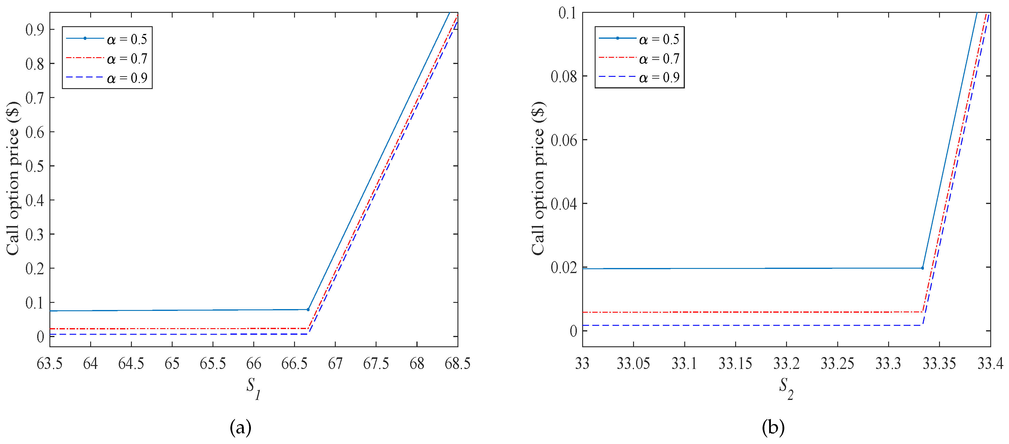
Figure 4. Solution plots of European call option obtained from the model with different orders $\alpha =0.5,0.7,0.9$ at a day before an expiration date: (a) $S_2=5$; (b) $S_1=10$.

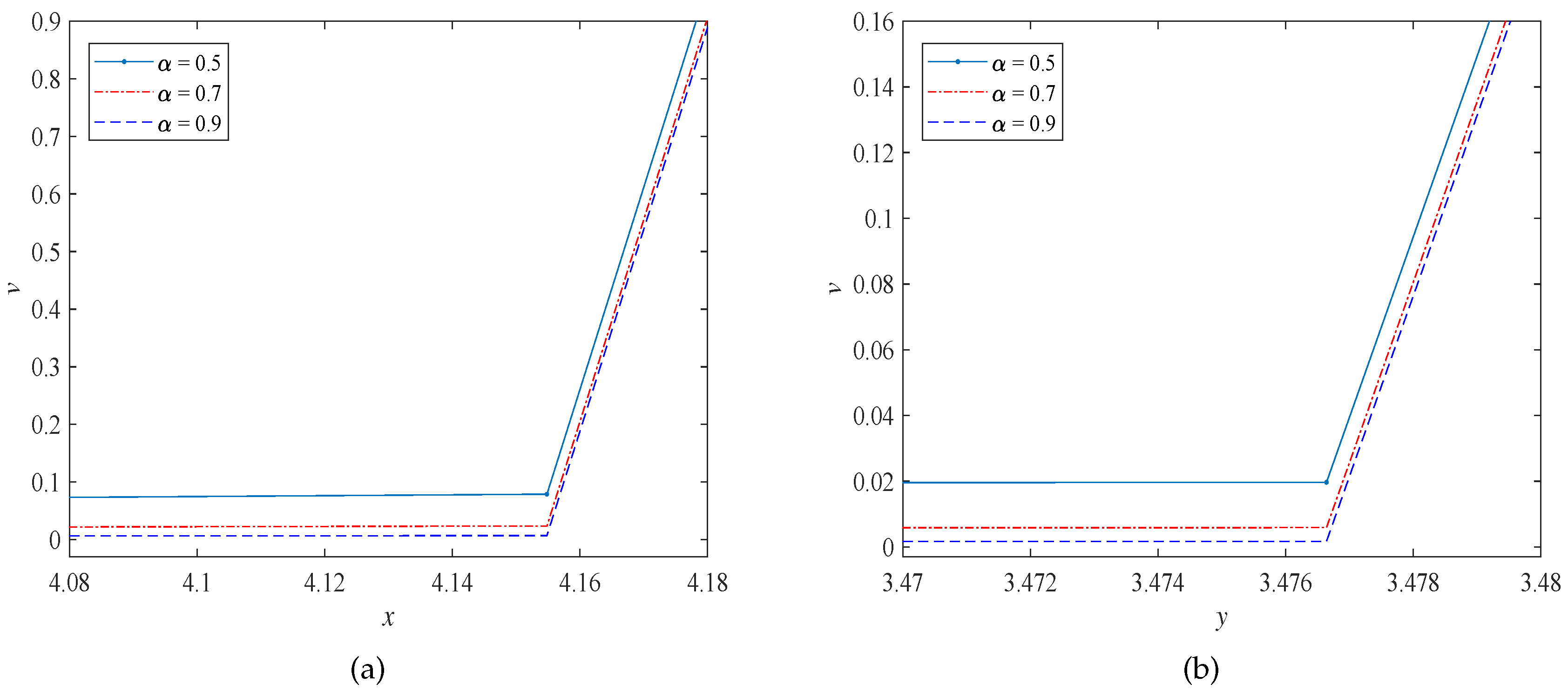
Figure 5. Solution v plots obtained from the model with different orders $\alpha =0.5,0.7,0.9$ at a day before an expiration date: (a) $y=1.6093$; (b) $x=2.3024$.

By setting $S_2=10$, the solutions v and c with order $\alpha =0.9$ are plotted in Figure 2a,b. With increasing $S_1$ from 0 to 50, the option price c reaches to zero. It is similar to c, v also reaches to zero when x increases from 2 to 4. The option price c increases linearly when the stock price is greater than 50. The solution v increases exponentially when x is greater than 4.

Figure 3 shows the surface plot of call option with $S_1=10$ over a range of stock price $0\le S_2\le 200$ and time $0\le t\le 1$. With increasing $S_2$ from 0 to 40, the option price c reaches to zero. v also reaches to zero when x increase from 2 to $3.8$. After that the option price c increases linearly when stock price is greater than 40. The solution v increases exponentially when x is greater than $3.8$.

At a day before an expiration date, the European call option price over the stock price $S_1$ and $S_2$ for various order $\alpha =0.5,0.7$ and $0.9$ is investigate. Effects of fractional order $\alpha$ on c for different orders when $S_2=5$ and $S_1=10$ are shown in Figure 4a,b, respectively. The comparison indicates that a higher order $\alpha$ gives a lower call option price. In Figure 5, the solution plot of v is similar trend to c. It is noted that a higher order $\alpha$ gives a lower option price v. Moreover, the option prices v increases rapidly after $x=4.2452$ and $y=3.4589$ as shown in Figure 5a,b, respectively. Consequently, we can conclude that the effect of time derivative order $\alpha$ has a small effect on the option price.

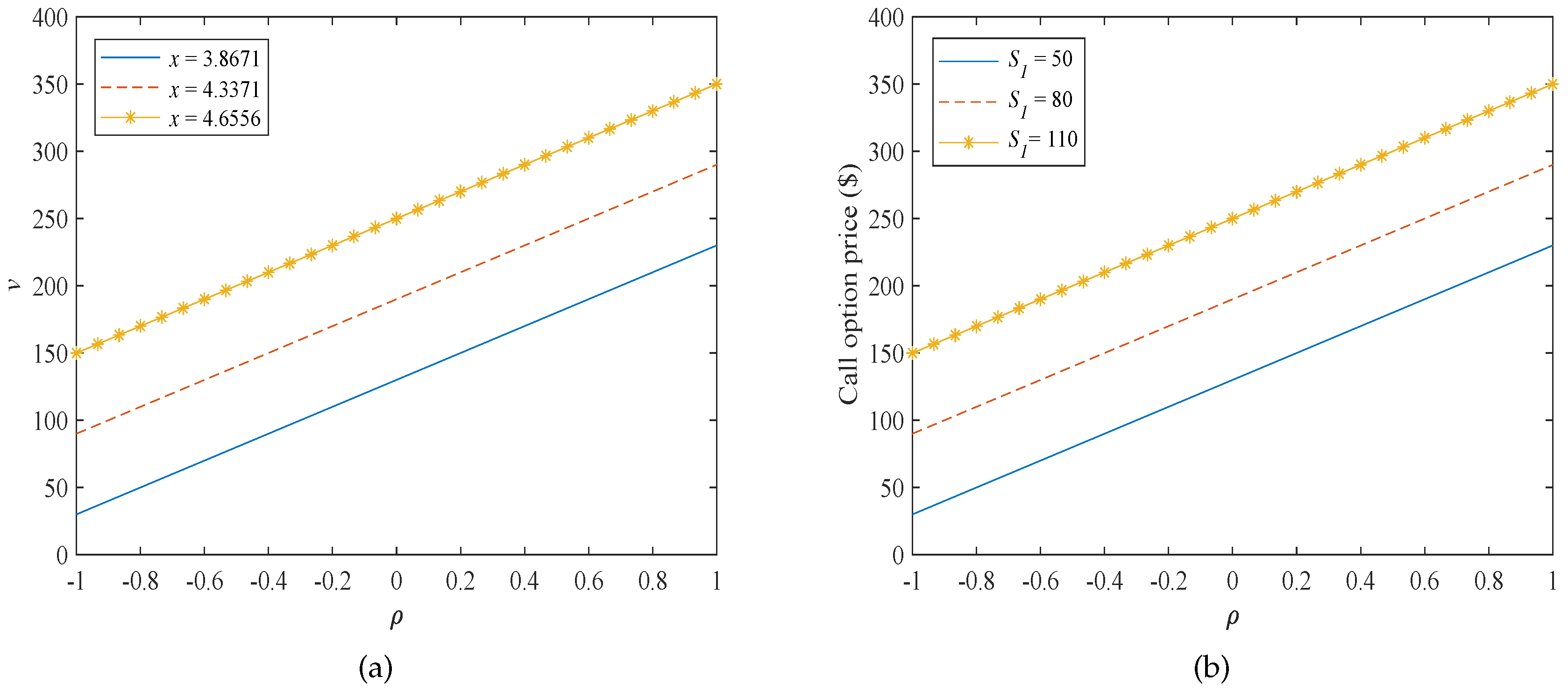
The values of European call option with the correlation varying from $-1$ to 1 is presented in Figure 6 at a day before an expiration date. The effects of stock price $S_2$ with some fixed stock prices $S_1$ and y with some fixed value x are investigated. Three values of $S_1$ including 50, 80 and 100 and three values of x including 3.8671, 4.3371 and 4.6556 are chosen for $S_2=5$ and $y=1.6093$. The result shows that the relationship between the European call option and the correlation is the increasing linear pattern. In addition, the rate of change of European call options v and c with respect to $\rho$ are also similar to each other as shown in Figure 6a,b.

Figure 6. Relationship between the European call option and the correlation $\rho$ for time derivative order $\alpha =0.9$ at a day before the expiration date: (a) v for $y=1.6093$ and (b) c for $S_2=5$.

5. Conclusions

The fractional Black-Scholes equations is a generalized version of the classical model which extend the restriction of using the model for finding the option price. As shown in the result, you can see that if parameters were not changed in the model, we obtain the difference value of option price with the different order. As a result, the fractional Black-Scholes model is more practical than the integer order model. This work introduced the Laplace homotopy perturbation method in order to find the explicit solution in time-fractional Black-Scholes model with two assets. By using the LHPM, the explicit solution can be written in the form of a special function, generalized Mittag-Leffer function. The benefit of the explicit solution form is easy to use for finding the European call option which depends on two stock price. Moreover, the numerical examples of the solution are presented to illustrate the explicit solution.

References

- Corzo, T.; Prat, M.; Vaquero, E. Behavioral Finance in Joseph de la Vega’s Confusion de Confusiones. J. Behav. Financ. 2014, 15, 341–350. [Google Scholar] [CrossRef]
- Osborne, M.F.M. Brownian motion in the stock market. Oper. Res. 1959, 7, 145–173. [Google Scholar] [CrossRef]
- Black, F.; Scholes, M. The pricing of options and corporate liabilities. J. Political Ecol. 1973, 81, 637–654. [Google Scholar] [CrossRef]
- Cen, Z.; Le, A. A robust finite difference scheme for pricing american put options with singularity-separating method. Numer. Algorithms 2010, 53, 497–510. [Google Scholar] [CrossRef]
- Cen, Z.; Le, A. A robust and accurate finite difference method for a generalized Black—Scholes equation. J. Comput. Appl. Math. 2011, 235, 2728–2733. [Google Scholar] [CrossRef]
- Kleinert, K.; Korbel, J. Option pricing beyond Black–Scholes based on double-fractional diffusion. J. Phys. A 2016, 449, 200–214. [Google Scholar] [CrossRef]
- Vazquez, C. An upwind numerical approach for an American and European option pricing model. Appl. Math. Comput. 1998, 97, 273–286. [Google Scholar] [CrossRef]
- Marcozzi, M.D.; Choi, S.; Chen, C.S. On the use of boundary conditions for variational formulations arising in financial mathematics. Appl. Math. Comput. 2001, 124, 197–214. [Google Scholar] [CrossRef]
- Kim, J.; Kim, T.; Jo, J.; Choi, Y.; Lee, S.; Hwang, H.; Yoo, M.; Jeong, D. A practical finite difference method for the three-dimensional Black–Scholes equation. Eur. J. Oper. Res. 2016, 252, 183–190. [Google Scholar] [CrossRef]
- Lesmana, D.C.; Wang, S. An upwind finite difference method for a nonlinear Black–Scholes equation governing European option valuation under transaction costs. J. Appl. Math. Comput. 2013, 219, 8811–8828. [Google Scholar] [CrossRef]
- Song, L.; Wang, W. Solution of the fractional Black–Scholes option pricing model by finite difference method. Abstr. Appl. Anal. 2013, 1–10. [Google Scholar] [CrossRef]
- Phaochoo, P.; Luadsong, A.; Aschariyaphotha, N. The meshless local Petrov–Galerkin based on moving kriging interpolation for solving fractional Black–Scholes model. J. King Saud Univ.-Sci. 2016, 28, 111–117. [Google Scholar] [CrossRef]
- Yoon, J.H. Mellin Transform Method for European Option Pricing with Hull-White Stochastic Interest Rate. J. Appl. Math. 2014, 2014, 759562. [Google Scholar] [CrossRef]
- He, J.H. Homotopy perturbation method for bifurcation of nonlinear problems. Int. J. Nonlinear Sci. Numer. Simul. 2005, 6, 207–208. [Google Scholar] [CrossRef]
- He, J.H. Homotopy perturbation technique. Comput. Methods Appl. Mech. Eng. 1999, 178, 257–262. [Google Scholar] [CrossRef]
- Trachoo, K.; Sawangtong, W.; Sawangtong, P. Laplace Transform Homotopy Perturbation Method for the Two Dimensional Black Scholes Model with European Call Option. Math. Comput. Appl. 2017, 22, 23. [Google Scholar] [CrossRef]
- Safdari-Vaighani, A.; Heryudono, A.; Larsson, E. A Radial Basis Function Partition of Unity Collocation Method for Convection–Diffusion Equations Arising in Financial Applications. J. Sci. Comput. 2015, 64, 341–367. [Google Scholar] [CrossRef]
- Shcherbakov, V.; Larsson, E. Radial basis function partition of unity methods for pricing vanilla basket options. Comput. Math. Appl. 2016, 71, 185–200. [Google Scholar] [CrossRef]
- Cavoretto, R.; Rossi, A.D.; Perracchione, E. Optimal Selection of Local Approximants in RBF-PU Interpolation. Download PDF J. Sci. Comput. 2018, 74, 1–22. [Google Scholar] [CrossRef]
- Cavoretto, R.; Schneider, T.; Zulian, P. OPENCL Based Parallel Algorithm for RBF-PUM Interpolation. J. Sci. Comput. 2018, 74, 267–289. [Google Scholar] [CrossRef]
- Bastian-Pinto, C.L. Modeling generic mean reversion processes with a symmetrical binomial lattice applications to real options. Procedia Comput. Sci. 2015, 55, 764–773. [Google Scholar] [CrossRef]
- Cox, J.C.; Ross, S. Rubinstein M. Option pricing: A simplified approach. J. Financ. Econ. 1949, 7, 229–263. [Google Scholar] [CrossRef]
- Glazyrina, A.; Melnikov, A. Bernstein’s inequalities and their extensions for getting the Black–Scholes option pricing formula. J. Stat. Probab. Lett. 2016, 111, 86–92. [Google Scholar] [CrossRef]
- Bjork, T.; Hult, H. A note on Wick products and the fractional Black–Scholes model. Financ. Stoch. 2005, 9, 197–209. [Google Scholar] [CrossRef]
- Kumar, S.; Kumar, D.; Singh, J. Numerical computation of fractional Black–Scholes equation arising in financial market. Egypt. J. Basic Appl. Sci. 2014, 1, 177–183. [Google Scholar] [CrossRef]
- Meng, L.; Wang, M. Comparison of Black–Scholes Formula with Fractional Black–Scholes Formula in the Foreign Exchange Option Market with Changing Volatility. Asia-Pac. Financ. Mark. 2010, 17, 99–111. [Google Scholar] [CrossRef]
- Misirana, M.; Lub, Z.; Teo, K.L. Fractional black-scholes models: complete mle with application to fractional option pricing. In Proceedings of the International Conference on Optimization and Control 2010, Guiyang, China, 18–23 July 2010; pp. 573–588. [Google Scholar]
- Mehrdoust, F.; Najafi, A.R. Pricing European Options under Fractional Black–Scholes Model with a Weak Payoff Function. Comput. Econ. 2017. [Google Scholar] [CrossRef]
- Jumarie, G. Derivation and solutions of some fractional Black–Scholes equations in coarse-grained space and time. Application to Merton’s optimal portfolio. Comput. Math. Appl. 2010, 59, 1142–1164. [Google Scholar] [CrossRef]
- Liu, H.K.; Chang, J.J. A closed-form approximation for the fractional Black–Scholes model with transaction costs. Comput. Math. Appl. 2013, 65, 1719–1726. [Google Scholar] [CrossRef]
- Zhang, H.; Liu, F.; Turner, I.; Yang, Q. Numerical solution of the time fractional Black–Scholes model governing European options. Comput. Math. Appl. 2016, 71, 1772–1783. [Google Scholar] [CrossRef]
- Contreras, M.; Llanquihuén, A.; Villena, M. On the Solution of the Multi-Asset Black-Scholes Model: Correlations, Eigenvalues and Geometry. J. Math. Financ. 2016, 6, 562–579. [Google Scholar] [CrossRef]
- Miller, K.S.; Ross, B. An Introduction Fractional Calculus Functional Differential Equations; Johan Willey and Sons Inc.: New York, NY, USA, 2003. [Google Scholar]
- Baholian, E.; Azizi, A.; Saeidian, J. Some notes on using the homotopy perturbation method for solving time-dependent differential equations. Math. Comput. Model. 2009, 50, 213–224. [Google Scholar] [CrossRef]
- Mathai, A.M.; Haubold, H.J. Mathematical Methods in the Applied Sciences; Springer: New York, NY, USA, 2008. [Google Scholar]
© 2018 by the authors. Licensee MDPI, Basel, Switzerland. This article is an open access article distributed under the terms and conditions of the Creative Commons Attribution (CC BY) license (http://creativecommons.org/licenses/by/4.0/).