1. Introduction
In recent years, the development of metaheuristics [
1,
2,
3] has advanced. Many scholars have made a lot of contributions in this area. The Artificial Bee Colony algorithm (ABC) [
4] is a novel swarm intelligence algorithm among the sets of metaheuristics. The ABC algorithm is an optimization algorithm which mimics the foraging behavior of the honey bee. It provides a population-based search procedure in which individuals called food positions are modified by the artificial bees with the increasing of iterations. The bee’s aim is to discover the places of food sources with high nectar amount.
From 2007 to 2009, Karaboga et al. [
5,
6,
7] presented a comparative study on optimizing a large set of numerical test functions. They compared the performance of the ABC algorithm with the genetic algorithm (GA), particle swarm optimization (PSO), differential evolution (DE) and evolution strategy (ES). The simulation results show that ABC can be efficiently employed to solve engineering problems with high dimensions. It can produce very good and effective results at a low computational cost by using only three control parameters (population size, maximum number of fitness evaluations, limit). Akay et al. [
8] studied the parameter tuning of the ABC algorithm and investigated the effect of control parameters. Afterwards, two modified versions of the ABC algorithm were proposed successively by Akay et al. [
9] and Zhang et al. [
10] for efficiently solving real-parameter numerical optimization problems. Aderhold et al. [
11] studied the influence of the population size about the optimization behavior of ABC and also proposed two variants of ABC which used the new position update of the artificial bees.
However, ABC was unsuccessful on some complex unimodal and multimodal functions [
7]. So, some modified artificial colony algorithms were put forward in order to improve the performance of the basic ABC. Zhu et al. [
12] proposed an improved ABC algorithm called gbest-guided ABC (GABC) by incorporating the information of global best solution into the solution search equation to guide the search of candidate solutions. The experimental results tested on six benchmark functions showed that GABC outperformed basic ABC. Wu et al. [
13] described an improved ABC algorithm to enhance the global search ability of basic ABC. Guo et al. [
14] presented a novel search strategy and the improved algorithm is called global ABC which has great advantages of convergence property and solution quality. In 2013, Yu et al. [
15] proposed a modified artificial bee colony algorithm in which global best is introduced to modify the update equation of employed and onlooker bees. Simulation results on the problem of peak-to-average power ratio reduction in orthogonal frequency division multiplexing signal and multi-level image segmentation showed that the new algorithm had better performance than the basic ABC algorithm with the same computational complexity. Rajasekhar et al. [
16] proposed a simple and effective variant of the ABC algorithm based on the improved self-adaptive mechanism of Rechenbergs 1/5th success rule to enhance the exploitation capabilities of the basic ABC. Yaghoobi [
17] proposed an improved artificial bee colony algorithm for global numerical optimization in 2017 from three aspects: initialising the population based on chaos theory; utilising multiple searches in employee and onlooker bee phases; controlling the frequency of perturbation by a modification rate.
Multi-objective evolutionary algorithms (MOEAs) gained wide attention to solve various optimization problems in fields of science and engineering. In 2011, Zou et al. [
18] presented a novel algorithm based on ABC to deal with multi-objective optimization problems. The concept of Pareto dominance was used to determine the flight direction of a bee, and the nondominated solution vectors which had been found in an external archive were maintained in the proposed algorithm. The proposed approach was highly competitive and was a viable alternative to solve multi-objective optimization problems.
The performances of Pareto-dominance based MOEAs degrade if the number of objective functions is greater than three. Amarjeet et al. [
19] proposed a Fuzzy-Pareto dominance driven Artificial Bee Colony (FP-ABC) to solve the many-objective software module clustering problems (MaSMCPs) effectively and efficiently in 2017. The contribution of the article was as follows: the selection process of candidate solution was improved by fuzzy-Pareto dominance; two external archives had been integrated into the ABC algorithm to balance the convergence and diversity. A comparative study validated the supremacy of the proposed approach compared to the existing many-objective optimization algorithms.
A decomposition-based ABC algorithm [
20] was also proposed to handle many-objective optimization problems (MaOPs). In the proposed algorithm, an MaOP was converted into a number of subproblems which were simultaneously optimized by a modified ABC algorithm. With the help of a set of weight vectors, a good diversity among solutions is maintained by the decomposition-based algorithm. The ABC algorithm is highly effective when solving a scalar optimization problem with a fast convergence speed. Therefore, the new algorithm can balance the convergence and diversity well. Moreover, subproblems in the proposed algorithm were handled unequally, and computational resources were dynamically allocated through specially designed onlooker bees and scout bees, which indeed contributed to performance improvements of the algorithm. The proposed algorithm could approximate a set of well-converged and properly distributed nondominated solutions for MaOPs with the high quality of solutions and the rapid running speed.
The basic ABC algorithms is often combined with other algorithms and techniques. In 2016, an additional update equation [
21] for all ABC-based optimization algorithms was developed to speed up the convergence utilizing Bollinger bands [
22] which is a technical analysis tool to predict maximum or minimum future stock prices. Wang et al. [
23] proposed a hybridization method based on krill herd [
24] and ABC (KHABC) in 2017. A neighbor food source for onlooker bees in ABC was obtained from the global optimal solutions, which was found by the KHABC algorithm. During the information exchange process, the globally best solutions were shared by the krill and bees. The effectiveness of the proposed methodology was tested for the continuous and discrete optimization.
In this paper, another technique called cloud model [
25] will be embedded into the ABC algorithm. Cloud model is an uncertainty conversion model between a qualitative concept and its quantitative expression. In 1999, an uncertainty reasoning mechanism of the cloud model was presented and the cloud model theory was be expanded after that. In addition, Li successfully applied cloud model to inverted pendulum [
26]. Some scholars combined cloud model with ABC because cloud model has the characteristics of stable tendentiousness and randomness [
27,
28,
29].
We propose a new algorithm which inherits the excellent exploration ability of the basic ABC algorithm and the stability and randomness of the cloud model by modifying the selection mechanism of onlookers, the search formula of onlookers and scout bees’ update formula. The innovation points of the new algorithm are:
The population becomes more diverse in the whole search process by using a different selection mechanism of onlookers, in which the worse individual will have a larger selection probability than in basic ABC;
Local search ability of the algorithm can be improved by applying the normal cloud generator as the search formula of onlookers to control the search of onlookers in a suitable range;
Historical optimal solutions can be used by Y-conditional cloud generator as scout bees’s update formula to ensure that the algorithm not only jumps out of local optimum but also avoids a blind random search.
The remainder of the paper is structured as follows.
Section 2 provides the description of the basic ABC algorithm, followed by the details and framework of the developed ABC algorithm based on cloud model, as shown in
Section 3. Subsequently,
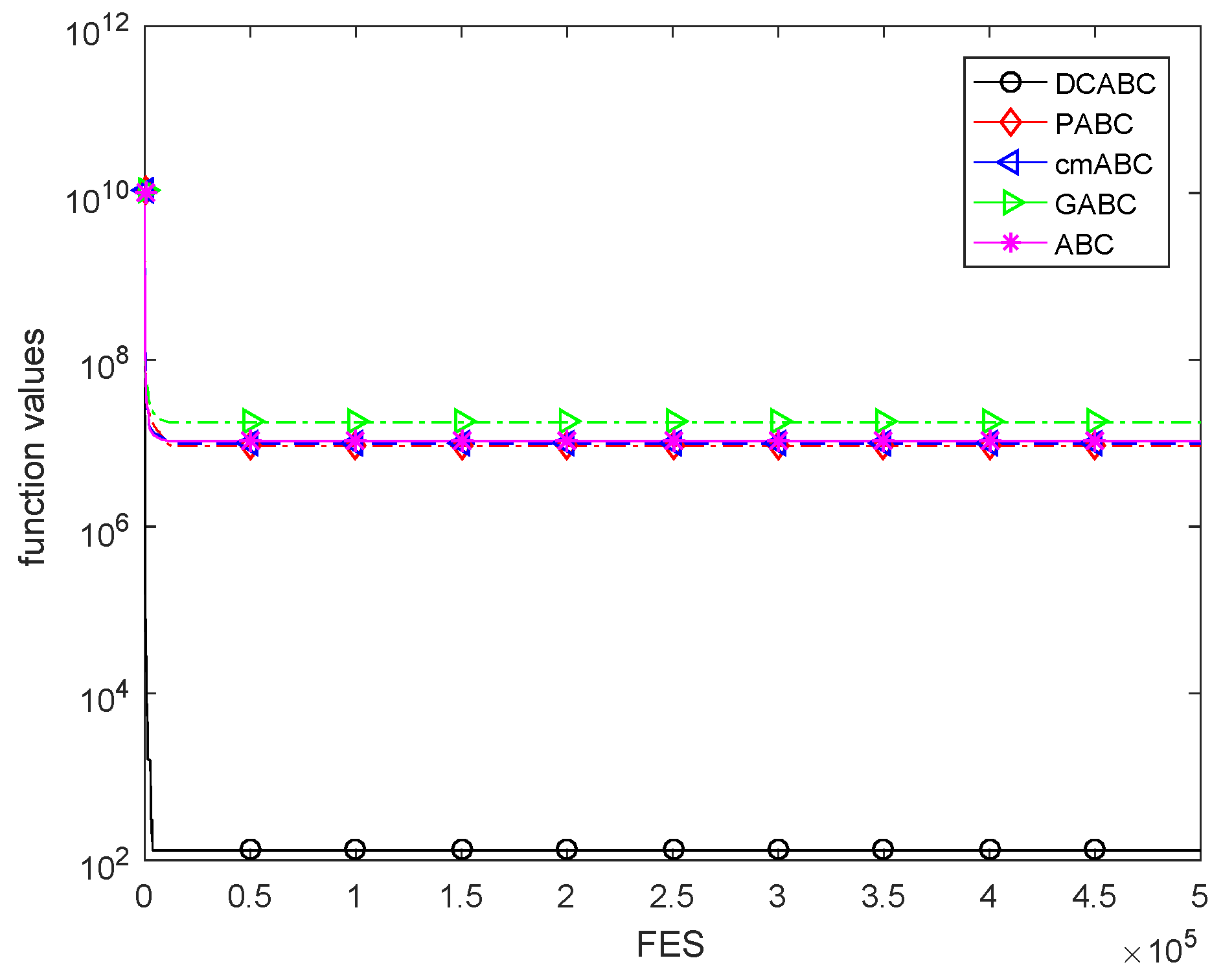
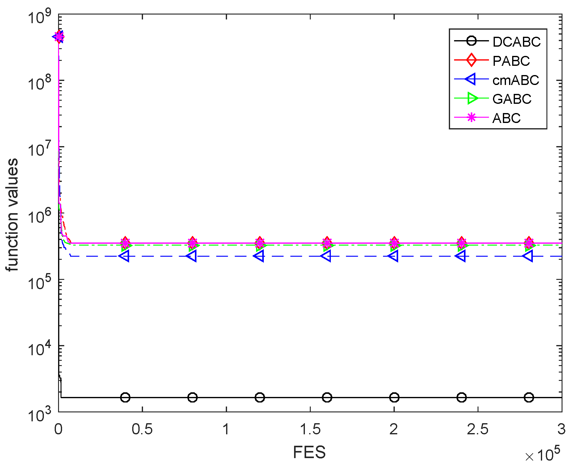
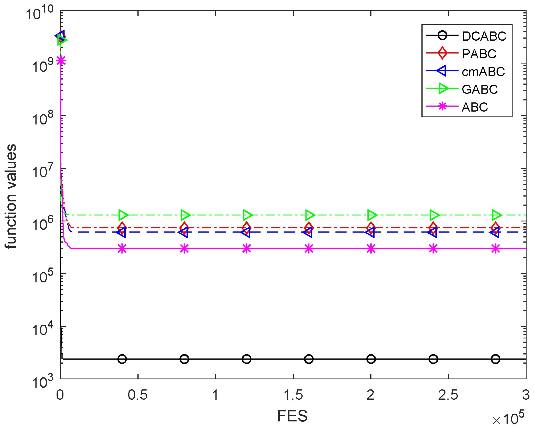
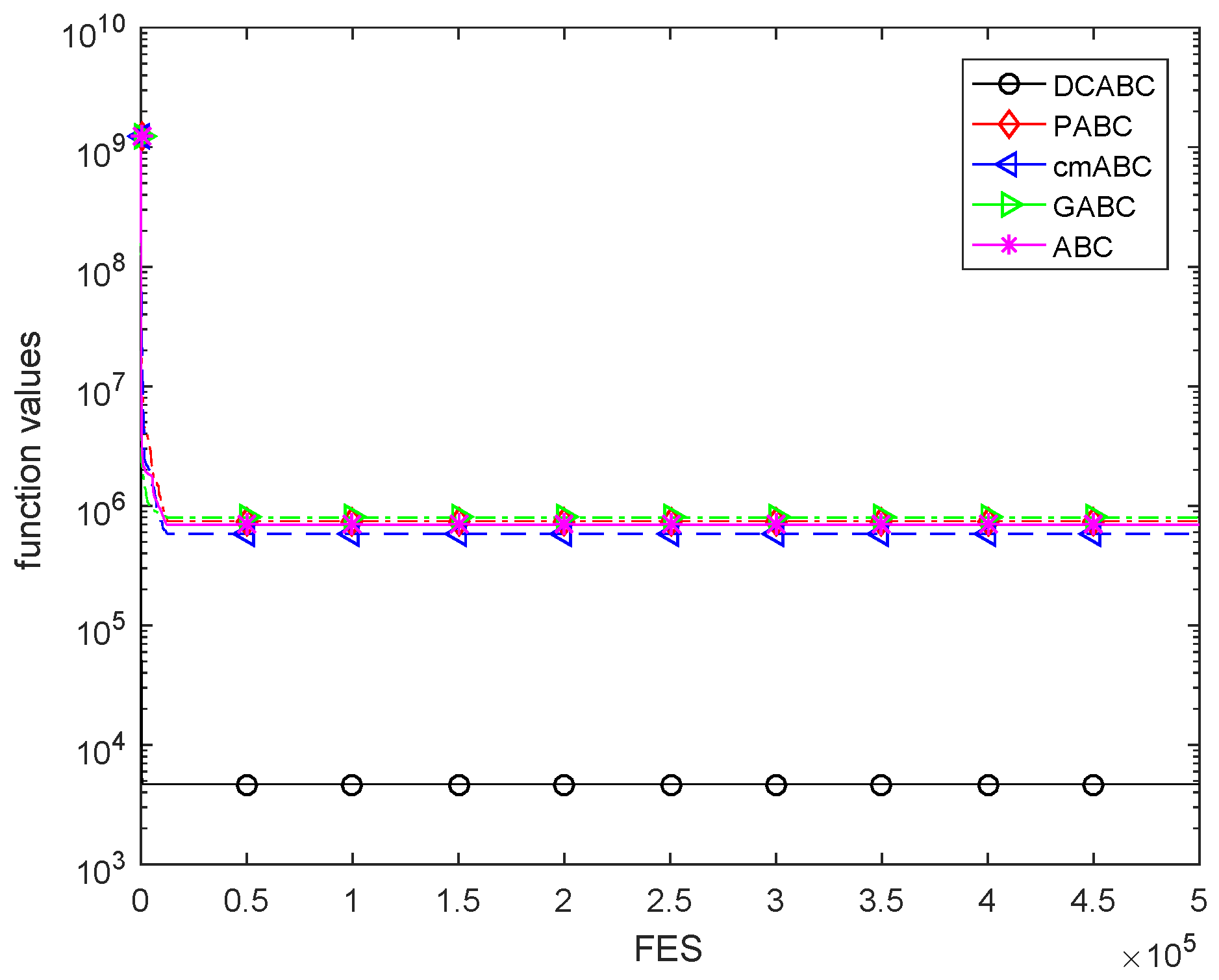
Section 4 gives the experiment results on CEC15 of the comparison among the proposed DCABC, the basic ABC, and other ABC variants based on cloud model. Then in
Section 5, the current work is summarized, and the acknowledgements are given in the end.
2. The Basic ABC Algorithm
There are three kinds of bees, namely, employed bees, onlooker bees and scout bees in the ABC algorithm. The total population number is
; the number of employed bees is
and onlookers is
(General define
). In the initialization phase, food sources in the population are randomly generated and assigned to employed bees as
where
,
are the upper and lower bounds of the solution vectors,
D is the dimension of the decision variable.
Each employed bee
generates a new food source
in the neighborhood of its present position:
where
,
,
k must be different from
i,
k and
j are random generating indexes,
is a random number between [−1, 1]. At the same time, we should guarantee
in the field of definition domain.
will be compared to
and the employed bee exploits the better food source by greedy selection mechanism in terms of fitness value
in Equation (
3):
where
is the objective value of solution
or
. Equation (
3) is used to calculate fitness values for a minimization problem, while for maximization problems the objective function can be directly used as a fitness function.
An onlooker bee evaluates the fitness value of all employed bees, and uses the roulette wheel method to select a food source
updated the same as employed bees according to its probability value
P calculated by the following expression:
If a food source
cannot be improved beyond a predetermined number (
limit) of trial counters, it will be abandoned and the corresponding employed bee will become a scout bee randomly produced by Equation (
1). The algorithm will be terminated after repeating a predefined maximum number of cycles, denoted as
. The flow chart of ABC algorithm is shown in Algorithm 1.
| Algorithm 1: The basic ABC algorithm. |
| Initialization phase |
| Initialize the food sources using Equation (1). |
| Evaluate the fitness value of the food sources using Equation (3), set the current generation . |
| While do |
| Employed bees phase |
| Send employed bees to produce new solutions via Equation (2). |
| Apply greedy selection to evaluate the new solutions. |
| Calculate the probability using Equation (4). |
| Onlooker bees phase |
| Send onlooker bees to produce new solutions via Equation (2). |
| Apply greedy selection to evaluate the new solutions. |
| Scout bee phase |
| Send one scout bee produced by Equation (1) into the search area for discovering a new food source. |
| Memorize the best solution found so far. |
| . |
| end while |
| Return the best solution. |
3. A Developed Artificial Bee Colony Algorithm Based on Cloud Model (DCABC)
The ABC algorithm is a relatively new and mature swarm intelligence optimization algorithm. Compared to GA and PSO, ABC has a higher robustness [
6]. More and more scholars want to improve the performance of the ABC algorithm. Zhang [
27] put forward an algorithm named PABC with the new select scheme based on cloud model. For the individual with a better fitness characteristic, the value of probability was likely relatively high, and vice versa. Lin et al. [
29] proposed an improved ABC algorithm based on cloud model (cmABC) to solve the problem that the basic ABC algorithm suffered from slow convergence and easy stagnation in local optima by calculating food source through the normal cloud particle operator and reducing the radius of the local search space. In cmABC, the author also introduced a new selection strategy that made the inferior individual have more chances to be selected for maintaining diversity. In addition, the best solution found over time was used to explore a new position in the algorithm. A number of experiments on composition functions showed that the proposed algorithm had been improved in terms of convergence speed and solution quality. In this section, we propose a developed ABC algorithm named DCABC which is based on cloud model with a new choice mechanism of onlookers and new search strategies of onlooker bees and scouts.
3.1. Cloud Model
Professor Li presented an uncertainty conversion model between a qualitative concept
[
30] presented by nature language and its quantitative expression which is called cloud model on the basis of traditional fuzzy set theory and probability statistics. He developed and improved a complete set of cloud theory [
31] which consists of cloud model, virtual cloud, cloud operations, cloud transform, uncertain reasoning and so on.
Suppose
U is a quantitative domain of discourse that are represented by precise values (one-dimensional, two-dimensional or multi-dimensional), and
is a qualitative concept in
U.
X is an arbitrary element in
U and a random implementation of qualitative concept
. The degree of certainty of
X to
expressed as
is an random number that has stable tendency. The distribution of
X on the domain of discourse
U is called cloud model, or simply ‘cloud’ for short. Each pare (
X,
) is called a cloud droplet, and cloud model can be formulated as follows:
The normal cloud is scattered point cloud model based on normal distribution or half-normal distribution. Normal cloud model uses a set of independent parameters to work together in order to express digital characteristics of a qualitative concept and reflect the uncertainty of the concept. Based on the normal distribution function and membership function, this group of parameters are represented by three digital characteristics including expectation , entropy , and hyper entropy .
Expectation is a point which can best represent the qualitative concept in domain of discourse space. It can be considered as the center of gravity of all cloud drop, which can best represent the coordinates of the qualitative concept on number field. Entropy stands for the measurable granularity of the qualitative concept. Entropy also reflects the uncertainty and fuzzy degree of the qualitative concept. Fuzzy degree means value range that can be accepted by the qualitative concept in domain of discourse. Hyper entropy is the measure of entropy’s uncertainty, namely entropy of . It reflects randomness of samples which represent qualitative concept values, and reveals the relevance of fuzziness and randomness. Hyper entropy can also reflect the aggregation extent of cloud droplets.
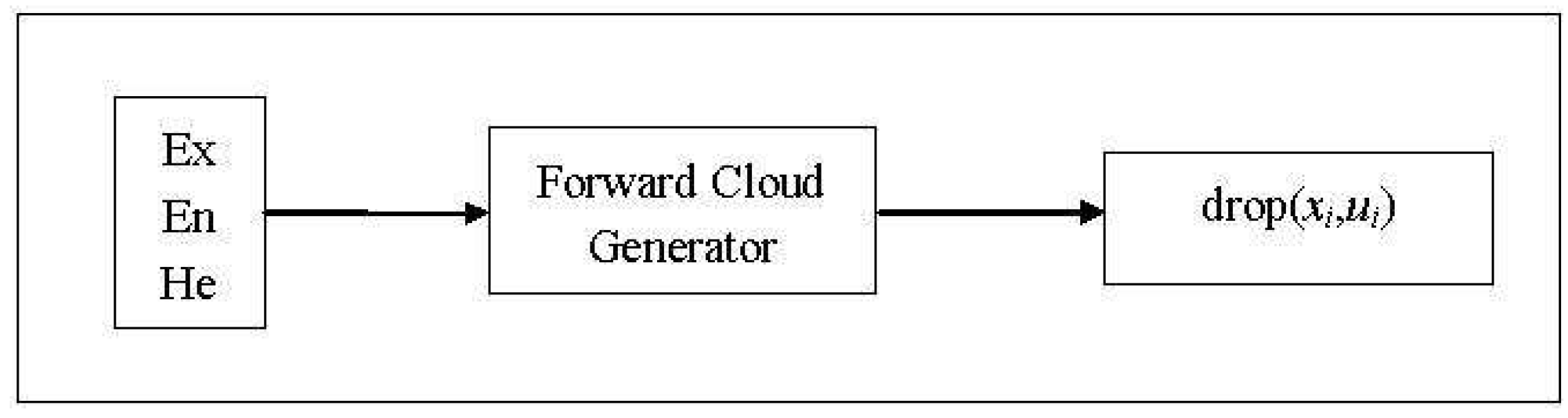
Given three digital characteristics
,
and
, forward cloud generator in Equations (
6)–(
8) can produce
N cloud droplets of the normal cloud model (Algorithm 2), which are two-dimensional points
(
).
| Algorithm 2: Forward cloud generator algorithm. |
| , , and N. |
| quantitative value of ith cloud droplet and its degree of certainty . |
| Forward cloud generator |
| Generate a normal random number with expectation and hyper entropy by Equation (6); |
| Generate a normal random number with expectation and hyper entropy by Equation (7). |
| Drop |
| Calculate by Equation (8); |
| A cloud droplet is get. |
| Repeat |
| Repeat the above step until N cloud droplets have come into being. (Figure 1) |
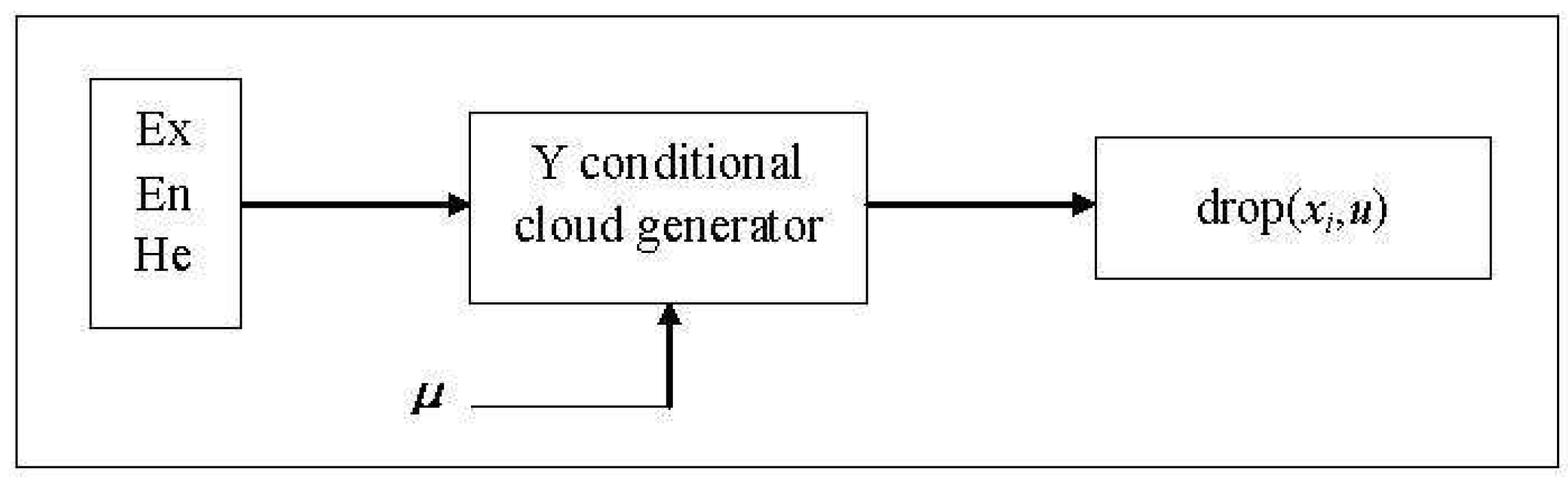
Given three digital characteristics (
) and a specific degree of certainty
, cloud generator refers to Y-conditional cloud generator based on uncertainty reasoning of cloud model. In other words, every cloud droplet(
,
) has the same degree of certainty which belongs to concept
. The formula of Y-conditional cloud generator (Algorithm 3) is:
| Algorithm 3: Y-conditional cloud generator algorithm. |
| , , , N and . |
| Quantitative values of ith cloud droplet and its degree of certainty . |
| Y-conditional cloud generator |
| Get a normal random number with expectation and hyper entropy by Equation (6); |
| Calculate with , and by Equation (9). |
| Drop |
| A Y-conditional cloud droplet is get. |
| Repeat |
| Repeat the above step until get N cloud droplets. (Figure 2) |
3.2. New Choice Mechanism for Onlookers
3.2.1. New Choice Mechanism
In the basic ABC algorithm, onlooker bees choose the good-quality nectars by employing the roulette wheel selection scheme. That is to say, the bigger the nectar’s fitness value, the higher the probability it will be chosen by onlookers. The selection mechanism contains three parts: calculating the selection probability of each solution in population according to its fitness value; selecting the candidate solution using the roulette wheel selection method; starting the local search of onlooker bees around the candidate solution. However, the selection scheme is so greedy that it is easy to lead to the rapid decrease of population diversity and fall into local optimum. We hope to obtain a reasonable selection scheme.
Zhang et al. [
27] improved the selection strategy based on cloud model with three digital characteristics
,
and
in Equation (
10):
The possibility of the current individual which is the best can be regarded as the choice probabilities and can be produced by the positive cloud generator. Thinking differently, it will be found that the worst individual also contains useful information after several loop iterations. So, we ensure that the worst individual has larger selection probability. Equation (
10) pays more attention to the inferior individuals. Detailed positive cloud generator operations can be described as follows:
The selective probability of the corresponding individual is adjusted as follows:
where,
,
, N is a normal random number generator.
We find that the individuals closer to Ex(inferior individuals) will get the higher possibility, namely, selection probability.
3.2.2. Efficiency Analysis
In our proposed algorithm DCABC, Equation (
4) is used as the probability selection formula for onlookers when a random number
between 0 and 1 are less than or equal to 0.5; otherwise the selection formula is set by the new choice mechanism in Equation (
12). The goal of processing selection probability in two cases is to avoid the algorithm plunging into local optimum.
To test the effectiveness of the current selection mechanism, the modified and the basic ABC run independently on CEC15 [
32] with dimensions(
D) 10, 30 and 50, respectively. We set the initial population size
. The number of employed bees equals to the number of onlookers, which is
. The value of ‘
’ equals to
[
33]. Every experiment is repeated 30 times. The maximum number of function evaluations (
) is set as
10,000 for all functions [
34]. The simulation results is recorded in
Table 1. It can be easily observed that the ABC with new choice mechanism is superior to the basic ABC on most functions. This implies that the new choice mechanism improves the performance of the basic ABC.
3.3. The New Search Strategy of Onlooker Bees
Lin et al. [
29] proposed an improved ABC algorithm based on cloud model (cmABC). By calculating a candidate food source through the normal cloud operator and reducing the radius of the local search, the cmABC algorithm was proved to enhance the convergence speed, exploitation capability and solution quality on the experiments of composition functions. In cmABC, three digital characteristics of cloud model
are given as:
where
is the current food sources position,
,
is variable. The forward cloud generator can produce a normal random number
, which will correspond to the new food sources position of
jth dimension. Detailed operations were described as:
The greater the value of entropy En, the wider the distribution of cloud droplets and vice versa. When the search iteration reached a certain number of times, the population was closer and closer to the optimal solution. A nonlinear decrease strategy to self-adaptive adjust the value of
was used in cmABC for the sake of improving the precision of solution and controlling the bees’ search range:
where
was the current number of iterations,
was the maximum number of cycles. The values of parameters
and
were set to 5 and
, respectively. In order not to specify too many parameters, in this paper, three digital characteristics of cloud model
are given as
where
,
,
k must be different from
i,
k,
j are random generating indexes. This amendment is based on the stable tendency and randomness of normal cloud model. The entropy
is selected by ‘
’ principle of normal cloud model, which can control the onlooker bees to search in a suitable range.
3.4. Search Strategy of Scouts Combined with Y Conditional Cloud Generator
Employed and onlooker bees look for a better food source around their neighborhoods in each cycle of the search. If the fitness value of a food source is not improved by a predetermined number of trials that is equal to the value of ‘
’, then that food source is abandoned by its employed bee and the employed bee associated with that food source becomes a scout bee. In the basic ABC, the scout randomly finds a new food source to replace the abandoned one by Equation (
2), which makes the convergence rate of the basic ABC slow for not taking full advantage of the historical optimal solution information. In this section we make the scout bee search a candidate position around the historical optimal value
(corresponding to
) by Y-conditional cloud operator. Search strategy of scouts combined with Y-conditional cloud generator is described in Algorithm 4. The purpose of setting
in Step 3 is to guarantee population diversity. Cloud droplets which have smaller membership degrees are farther from center
, that is to say the new food source is farther from historical optimum
. However, the historical optimum information is used to generate a scout, therefore aimless searching of scout bees in the basic ABC algorithm can be avoided to a certain degree.
| Algorithm 4: Search strategy of scouts combined with Y-conditional cloud generator. |
| Set expectation as , which is the position parameters of . |
| Entropy . |
| Hyper entropy , where . |
| Randomly generate membership degrees , where . |
| Obtain the new food resource according to Equation (9). |
3.5. DCABC Algorithm
Pseudo code of DCABC algorithm proposed for solving unconstrained optimization problems is given in Algorithm 5. represents the maximum number of function evaluations. represents the number of function evaluations.
| Algorithm 5: Pseudo code of DCABC algorithm. |
| Initialization phase |
| Using Equation (1) initialize the population of solutions , i = 1, 2,…,, j = 1, 2,…, D. |
| Evaluate the fitness of the population by Equation (3), set the current . |
| While do |
| Employed bees phase |
| Send employed bees to produce new solutions via Equation (2). |
| Apply greedy selection to evaluate the new solutions. |
| If less than or equal to 0.5, Calculate the selective probability using Equation (4); |
| Otherwise calculate the probability using Equations (11) and (12). |
| Onlooker bees phase |
| Send onlooker bees to produce new solutions via Equations (14) and (16). |
| Apply greedy selection to evaluate the new solutions. |
| Scout bee phase |
| Send one scout bee generated by Algorithm 4 into the search area for discovering a new food source. |
| Memorize the best solution found so far. |
| end while |
| Return the best solution. |
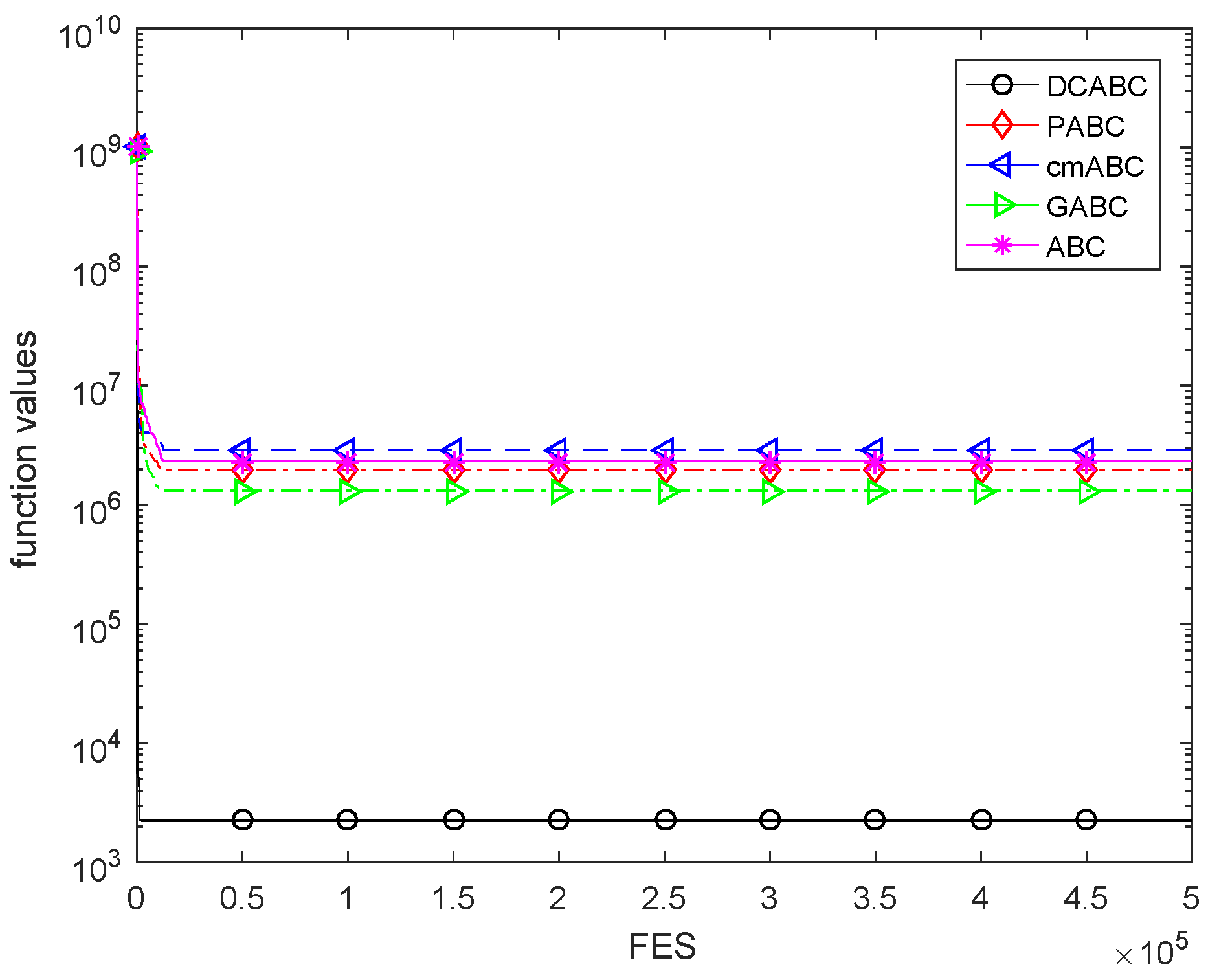
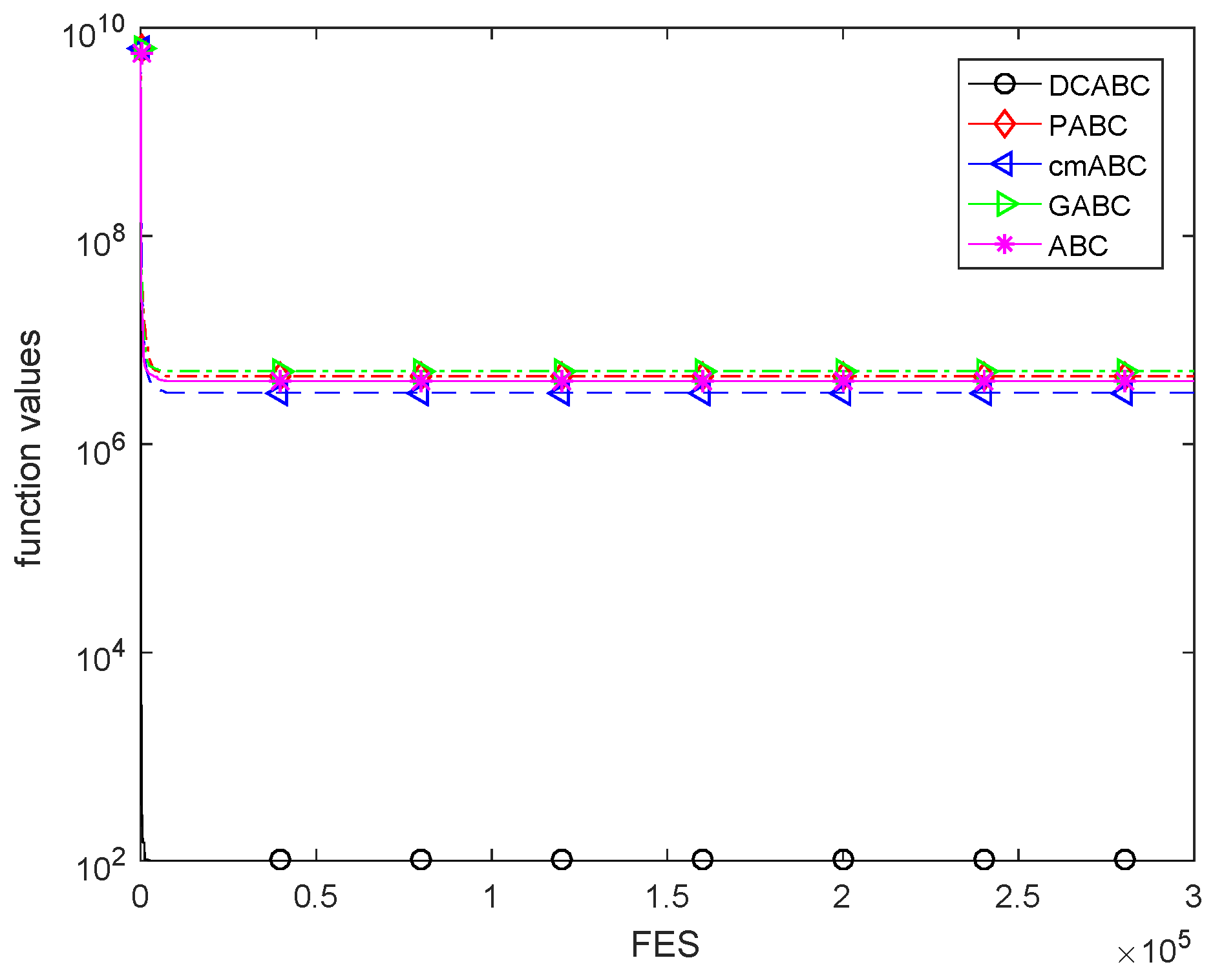
5. Conclusions
In the present study, a developed artificial bee colony algorithm based on cloud model, namely DCABC, is proposed for the continuous optimization. By using a new selection mechanism, the worse individual in DCABC has a larger probability to be selected than in basic ABC. DCABC also improves the local search ability by applying the normal cloud generator as onlookers bees’ formula to control the search of onlookers in a suitable range. Moreover, historical optimal solutions are used by Y conditional cloud generator when updating the scout bee to ensure the algorithm jump out of the local optimal. The effectiveness of the proposed method is tested on CEC15. The results clearly show the superiority of DCABC over ABC, GABC, cmABC and PABC.
However, there are quite a few issues that merit further investigation such as the diversity of DCABC. In addition, we hope to show the performance of DCABC by Null Hypothesis Significance Testing (NHST) [
35,
36] in our future work. We only test the new algorithm on classical benchmark functions and have not used it to solve practical problems, such as fault diagnosis [
37], path plan [
38], Knapsack [
39,
40,
41], multi-objective optimization [
42], gesture segmentation [
43], unit commitment problem [
44], and so on. There is an increasing interest in prompting the performance of DCABC, which will be our future research direction.


