Article

Serret-Frenet Frame and Curvatures of Bézier Curves

Department of Mathematics, Faculty of Arts and Sciences, Yildiz Technical University, 34220 Istanbul, Turkey
*
Author to whom correspondence should be addressed.
Mathematics 2018, 6(12), 321; https://doi.org/10.3390/math6120321
Submission received: 24 October 2018 / Revised: 24 November 2018 / Accepted: 5 December 2018 / Published: 12 December 2018

Abstract

:
The aim of this study is to view the role of Bézier curves in both the Euclidean plane E 2 and Euclidean space E 3 with the help of the fundamental algorithm which is commonly used in Computer Science and Applied Mathematics and without this algorithm. The Serret-Frenet elements of non-unit speed curves in the Euclidean plane E 2 and Euclidean space E 3 are given by Gray et al. in 2016. We used these formulas to find Serret-Frenet elements of planar Bézier curve at the end points and for every parameter t. Moreover, we reconstruct these elements for a planar Bézier curve, which is defined by the help of the algorithm based on intermediate points. Finally, in the literature, the spatial Bézier curve only mentioned at the end points, so we improve these elements for all parameters t. Additionally, we calculate these elements for all parameters t using algorithm above mentioned for spatial Bézier curve.

1. Introduction

For ease of curve and surface design, mathematician Paul De Casteljau started research on a formula in 1959. With the same purpose, engineer Pierre Bézier developed a similar formula that was independent and unaware of his research. As a result of Bézier’s relevant studies published in 1968, the theory is known by his name. The Bézier’s formula, as a consequence of these studies, is based on the way of explaining an approximation to the original curve using the control points b 0 , b 1 , , b n that pertain to the ordered set in [1]. Hence, it responds to the behavior of its control points by following a push-pull effect [2].
To descend to particulars in the formula, we need to give a brief definition of a Bézier curve: it is a parametric curve P ( t ) of degree n with n + 1 control points and defined by
P ( t ) = i = 0 n B i , n ( t ) b i , 0 t 1
where the b i s represent the n + 1 control points in Euclidean space E n [3]. Namely, Bézier curves are given by a linear combination of basic functions named the Bernstein polynomials with vector-valued coefficients named poles or control points [2].
The theory of Bézier curves has a significant importance in Computer Aided Design (CAD), since they are numerically the most stable among all polynomial bases in CAD and give an ideal geometric representation for piecewise polynomial curves [4]. Piecewise polynomial curves or functions are often used to represent the approximate solution in the numerical solution of differential equations. The Bézier curves are used in solving partial differential equations, wave and heat equations, and dynamical systems [5].
Bézier curves are strong devices to build freeform curves in CAD/CAM. On the other hand, they have their own deficiency. Namely, when electing the basic functions, the shape of Bézier curve is well assigned by its control points. To counter this deficiency, many scientists built new curves similar to Bézier curves [6,7].
A Bézier curve that is parametric has a continuous curvature and is used in various executions such as medical and engineering fields. Building two pieces of a Bézier curve may be attractive regarding protecting continuity and satisfying a specific shape such as curvature and torsion [8]. The properties of differential invariants such asas the curvature and the torsion in Euclidean geometry are researched in articles [9,10,11]. We refer the reader interested in the curvature and torsion of a Bézier curve at only the end points and for their geometric meanings in the sense of differential geometry to references [4,12,13]. Additionally, in [14], there is a remarkable result related to the Serret-Frenet frame at the end points.
In our work, we investigate the Serret-Frenet elements of planar Bézier curves and examine those elements by using the definition of algorithmic planar Bézier curves. Finally, we give the Serret-Frenet elements of algorithmic spatial Bézier curves.

2. Preliminaries

In this section, some necessary definitions and essential theory related Serret-Frenet elements of the Bézier curve and the algorithmic Bézier curve in Euclidean plane E 2 and in Euclidean space E 3 are introduced.

2.1. Some Concepts for Bézier Curve

Definition 1.
The n-th degree Bézier curve P ( t ) with n + 1 control points is a parametric function and it is defined by
P ( t ) = i = 1 n B i , n ( t ) b i , 0 t 1
where coefficients b i ’s are control points in Euclidean space E n and B i , n ( t ) symbolizes the Bernstein polynomial given by
B i , n ( t ) = n i t i ( 1 t ) n i
with the binomial coefficient:
n i = n ! i ! ( n i ) ! , i = 0 , . . . , n .
See reference [1].
Definition 2.
Let b 0 , b 1 and b 2 be non-linear three points in E n . A Bézier curve having the equation
P 2 ( t ) = i = 0 2 B i , 2 ( t ) b i = B 0 , 2 ( t ) b 0 + B 1 , 2 ( t ) b 1 + B 2 , 2 ( t ) b 2 = ( 1 t ) 2 b 0 + 2 ( 1 t ) t b 1 + t 2 b 2
is called non-unit speed quadratic Bézier curve in E n with the control points b 0 , b 1 , b 2 [13].
Definition 3.
Let b 0 , b 1 , b 2 and b 3 be non-linear four points in E n . The Bézier curve P 3 ( t ) given by
P 3 ( t ) = i = 0 3 B i , 3 ( t ) b i = B 0 , 3 ( t ) b 0 + B 1 , 3 ( t ) b 1 + B 2 , 3 ( t ) b 2 + B 3 , 3 ( t ) b 3 = ( 1 t ) 3 b 0 + 3 ( 1 t ) 2 t b 1 + 3 ( 1 t ) t 2 b 2 + t 3 b 3
is called non-unit speed cubic Bézier curve in E n with the control points b 0 , b 1 , b 2 , b 3 [13].
Theorem 1.
The first order derivative of the n-th degree Bézier curve is
P ( t ) = n i = 0 n 1 B i , n 1 ( t ) Δ b i
where Δ b i is the difference equation defined by Δ b i = b i + 1 b i [13].
Corollary 1.
The second order derivative of the n-th degree Bézier curve is given by
P ( t ) = n ( n 1 ) i = 0 n 2 B i , n 2 ( t ) Δ 2 b i
where Δ 2 b i is difference equation described by Δ 2 b i = Δ b i + 1 Δ b i = b i + 2 2 b i + 1 + b i [13].
Corollary 2.
The r-th order derivative of the n-th degree Bézier curve is given by
P ( r ) ( t ) = n ! ( n r ) ! i = 0 n r B i , n r ( t ) Δ r b i
where Δ r b i is difference equation indicated by Δ r b i = Δ r 1 b i + 1 Δ r 1 b i = b i + 2 2 b i + 1 + b i [4,13].
Corollary 3.
The values of r-th order derivative of the n-th Bézier curve at the starting point and the ending point are given with the following equalities, respectively [4]:
P ( r ) ( t ) t = 0 = n ! ( n r ) ! Δ r b 0
and
P ( r ) ( t ) t = 1 = n ! ( n r ) ! Δ r b n r .

2.2. The Theory of Curves in E 2 and E 3

Definition 4.
Let J : E 2 E 2 be a linear transformation defined by
J ( p 1 , p 2 ) = ( p 2 , p 1 ) .
In other words, ( p 2 , p 1 ) is obtained by rotating ( p 1 , p 2 ) counter clockwise 90 degree from origin. For each p , q E 2 , if we have the following properties:
J p , J q = p , q
J p , p = 0
J p , q = p , J q .
then J is called as complex structure of E 2 [15].
Definition 5.
Let p and q be two non-zero vectors in E 2 . We define
cos θ = p , q p q
sin θ = p , J q p q .
where θ is a unique orientation angle from p to q such that 0 θ 2 π [15].
Definition 6.
Let α : I E 2 be a non-unit speed planar curve. The Serret-Frenet frame { T , N } and curvature κ of α for t I are defined by the following equations [15]:
T ( t ) = α ( t ) α ( t )
N ( t ) = J α ( t ) α ( t )
κ ( t ) = α ( t ) , J α ( t ) α ( t ) 3 .
Definition 7.
Let α : I E 3 be a non-unit speed curve. The Serret-Frenet frame { T , N , B } , curvature κ and torsion τ of α are defined by the following equations [15]:
T ( t ) = α ( t ) α ( t )
N ( t ) = B ( t ) × T ( t )
B ( t ) = α ( t ) × α ( t ) α ( t ) × α ( t )
κ ( t ) = α ( t ) × α ( t ) α ( t ) 3
τ ( t ) = d e t ( α ( t ) , α ( t ) , α ( t ) ) α ( t ) × α ( t ) 2 .

3. Serret-Frenet Elements of Bézier Curve in E 2

Serret-Frenet Elements of Bézier Curve of Degree n in E 2

Theorem 2.
The Serret-Frenet frame { T , N } and curvature κ of non-unit speed planar Bézier curve of degree n with control points b 0 , b 1 , , b n defined by (1) for t R are
T ( t ) = i = 0 n 1 B i , n 1 ( t ) Δ b i i , j = 0 n 1 B i , n 1 ( t ) B j , n 1 ( t ) Δ b i , Δ b j 1 / 2
N ( t ) = i = 0 n 1 B i , n 1 ( t ) J Δ b i i , j = 0 n 1 B i , n 1 ( t ) B j , n 1 ( t ) Δ b i , Δ b j 1 / 2
κ ( t ) = n 1 n i = 0 n 2 j = 0 n 1 B i , n 2 ( t ) B j , n 1 ( t ) Δ 2 b i , J Δ b j i , j = 0 n 1 B i , n 1 ( t ) B j , n 1 ( t ) Δ b i , Δ b j 3 / 2 .
Proof of Theorem 2.
The Serret-Frenet frame { T , N } is obtained using (4), (12), (13) as follows:
T ( t ) = P ( t ) P ( t ) = n i = 0 n 1 B i , n 1 ( t ) Δ b i n i = 0 n 1 B i , n 1 ( t ) Δ b i = i = 0 n 1 B i , n 1 ( t ) Δ b i i , j = 0 n 1 B i , n 1 ( t ) B j , n 1 ( t ) Δ b i , Δ b j 1 / 2 ,
N ( t ) = J P ( t ) P ( t ) = i = 0 n 1 B i , n 1 ( t ) J Δ b i i = 0 n 1 B i , n 1 ( t ) Δ b i = i = 0 n 1 B i , n 1 ( t ) J Δ b i i , j = 0 n 1 B i , n 1 ( t ) B j , n 1 ( t ) Δ b i , Δ b j 1 / 2 .
The curvature κ is obtained using (4), (5), (14) as follows:
κ ( t ) = P ( t ) , J P ( t ) ( P ( t ) , P ( t ) ) 3 / 2 = n 1 n i = 0 n 2 j = 0 n 1 B i , n 2 ( t ) B j , n 1 ( t ) Δ 2 b i , J Δ b j i , j = 0 n 1 B i , n 1 ( t ) B j , n 1 ( t ) Δ b i , Δ b j 3 / 2 .
Case 1.
The Serret-Frenet frame { T , N } and curvature κ of non-unit speed planar the n-th degree Bézier curve with the control points b 0 , b 1 , , b n are
T ( t ) t = 0 = Δ 1 b 0 Δ 1 b 0
N ( t ) t = 0 = J Δ 1 b 0 Δ 1 b 0
κ ( t ) t = 0 = n 1 n Δ 1 b 1 , J Δ 1 b 0 Δ 1 b 0 3 .
which is defined by (1) at t = 0
Proof of Case 1.
The value of Serret-Frenet frame { T , N } at t = 0 is obtained by considering t = 0 in Theorem 2 and r = 1 in (7). The curvature κ ( t ) is also calculated by disposing t = 0 in Theorem 2 and r = 1 , r = 2 in (7). We use the equalities Δ 2 b 0 = Δ 1 b 1 Δ 1 b 0 and (9) in above calculation.  □
After all, using (11) we get the formula for the curvature κ in the form of
κ ( t ) t = 0 = n 1 n Δ 1 b 1 Δ 1 b 0 2 sin α
where α is the angle between Δ 1 b 0 and Δ 1 b 1 .
Case 2.
The Serret-Frenet frame { T , N } and curvature κ of non-unit speed planar the n-th degree Bézier curve with control points b 0 , b 1 , , b n are
T ( t ) t = 1 = Δ 1 b n 1 Δ 1 b n 1
N ( t ) t = 1 = J Δ 1 b n 1 Δ 1 b n 1
κ ( t ) t = 1 = n 1 n Δ 1 b n 1 , J Δ 1 b n 2 Δ 1 b n 1 3 .
which is defined by (1) at t = 1 .
Proof of Case 2.
The value of Serret-Frenet frame { T , N } at t = 1 is obtained by considering t = 1 in Theorem 2 and r = 1 in (8). The curvature κ ( t ) is also calculated by disposing t = 1 in Theorem 2 and r = 1 , r = 2 in (8). We use the equalities Δ 2 b n 2 = Δ 1 b n 1 Δ 1 b n 2 , (9) and (10) in the above calculation. □
After all, using (11) we get the formula for the curvature κ in the form of
κ ( t ) t = 1 = n 1 n Δ 1 b n 2 Δ 1 b n 1 2 sin β
where β is the angle between Δ 1 b n 1 and Δ 1 b n 2 .
Case 3.
The Serret-Frenet frame { T , N } and curvature κ P 2 of non-unit speed planar quadratic Bézier curve with control points b 0 , b 1 and b 2 defined by (2) for t R are
T ( t ) = ( 1 t ) Δ 1 b 0 + t Δ 1 b 1 ( 1 t ) Δ 1 b 0 + t Δ 1 b 1
N ( t ) = ( 1 t ) J Δ 1 b 0 + t J Δ 1 b 1 ( 1 t ) Δ 1 b 0 + t Δ 1 b 1
κ P 2 ( t ) = 1 2 Δ 1 b 1 , J Δ 1 b 0 ( 1 t ) Δ 1 b 0 + t Δ 1 b 1 3 .
Proof of Case 3.
The first and second derivative of Bézier curve P 2 ( t ) given by (2), in terms of forward difference operators, are written as follows:
P 2 ( t ) = 2 ( 1 t ) ( 1 ) b 0 + ( 2 t b 1 + 2 ( 1 t ) b 1 ) + 2 t b 2 = 2 ( 1 t ) Δ 1 b 0 + 2 t Δ 1 b 1 ,
and
P 2 ( t ) = 2 Δ 1 b 0 + 2 t Δ 1 b 1 = 2 ( Δ 1 b 1 Δ 1 b 0 ) = 2 Δ 2 b 0 .
The Serret-Frenet frame { T , N } is obtained from (12) and (13) and the first derivative calculated above.
The curvature κ P 2 is derived using (9), (10), (14) and Δ 2 b 0 = Δ 1 b 1 Δ 1 b 0 . □
Case 4.
The Serret-Frenet frame { T , N } and curvature κ P 3 of non-unit speed planar cubic Bézier curve with control points b 0 , b 1 , b 2 and b 3 defined by (3) for t R are
T ( t ) = ( 1 t ) 2 Δ 1 b 0 + 2 ( 1 t ) t Δ 1 b 1 + t 2 Δ 1 b 2 ( 1 t ) 2 Δ 1 b 0 + 2 ( 1 t ) t Δ 1 b 1 + t 2 Δ 1 b 2
N ( t ) = ( 1 t ) 2 J Δ 1 b 0 + 2 ( 1 t ) t J Δ 1 b 1 + t 2 J Δ 1 b 2 ( 1 t ) 2 Δ 1 b 0 + 2 ( 1 t ) t Δ 1 b 1 + t 2 Δ 1 b 2
κ P 3 ( t ) = 2 3 ( 1 t ) 2 Δ 1 b 1 , J Δ 1 b 0 + ( 1 t ) t Δ 1 b 2 , J Δ 1 b 0 + t 2 Δ 1 b 2 , J Δ 1 b 1 ( 1 t ) 2 Δ 1 b 0 + 2 ( 1 t ) t Δ 1 b 1 + t 2 Δ 1 b 2 3 .
Proof of Case 4.
The first and second derivative of Bézier curve P 3 ( t ) given by (3) in terms of forward difference operators are written as follows:
P 3 ( t ) = 3 ( 1 t ) 2 ( 1 ) b 0 + 6 ( 1 t ) ( 1 ) t b 1 + 3 ( 1 t ) 2 b 1 3 t 2 b 2 + 6 ( 1 t ) t b 2 + 3 t 2 b 3 = 3 ( 1 t ) 2 Δ 1 b 0 + 6 ( 1 t ) t Δ 1 b 1 + 3 t 2 Δ 1 b 2
and
P 3 ( t ) = 6 ( Δ 1 b 1 Δ 1 b 0 ) + 6 t ( Δ 1 b 0 2 Δ 1 b 1 + Δ 1 b 2 )
The Serret-Frenet frame { T , N } is obtained from (12) and (13) and the first derivative which is calculated above.
Moreover, the curvature κ P 3 is derived using (9), (10), (14) and Δ 2 b 0 = Δ 1 b 1 Δ 1 b 0 .□

4. Serret-Frenet Elements of Bézier Curve in E 3

In this section, we give the Serret-Frenet elements of Bézier curve in E 3 for all points, in the case of t = 0 and t = 1 , we get the results given by [14].
Theorem 3.
The Serret-Frenet frame { T , N , B } , curvature κ and torsion τ of the non-unit spatial the n-th degree Bézier curve P ( t ) with control points b 0 , b 1 , , b n defined by (1) for t R are
T ( t ) = i = 0 n 1 B i , n 1 ( t ) Δ 1 b i i = 0 n 1 B i , n 1 ( t ) Δ 1 b i
B ( t ) = i = 0 n 1 j = 0 n 2 B i , n 1 ( t ) B j , n 2 ( t ) ( Δ 1 b i × Δ 2 b j ) i = 0 n 1 j = 0 n 2 B i , n 1 ( t ) B j , n 2 ( t ) ( Δ 1 b i × Δ 2 b j )
N ( t ) = i = 0 n 1 j = 0 n 2 k = 0 n 1 B i , n 1 ( t ) B j , n 2 ( t ) B k , n 1 ( t ) ( Δ 1 b i × Δ 2 b j ) × Δ b k i = 0 n 1 j = 0 n 2 k = 0 n 1 B i , n 1 ( t ) B j , n 2 ( t ) B k , n 1 ( t ) ( Δ 1 b i × Δ 2 b j ) × Δ b k
κ ( t ) = n 1 n i = 0 n 1 j = 0 n 2 B i , n 1 ( t ) B j , n 2 ( t ) ( Δ 1 b i × Δ 2 b j ) i = 0 n 1 B i , n 1 ( t ) Δ 1 b i 3
τ ( t ) = n 2 n i = 0 n 1 j = 0 n 2 k = 0 n 3 B i , n 1 ( t ) B j , n 2 ( t ) B k , n 3 ( t ) Δ 1 b i × Δ 2 b j , Δ 3 b k i = 0 n 1 j = 0 n 2 B i , n 1 ( t ) B j , n 2 ( t ) ( Δ 1 b i × Δ 2 b j ) 2 .
Proof of Theorem 3.
Using (15)–(19), (4) for the first derivative, (5) for the second derivative, and (6) for the third derivative; the Serret-Frenet elements { T , N , B , κ , τ } are obtained as follows:
T ( t ) = P ( t ) P ( t ) = n i = 0 n 1 B i , n 1 ( t ) Δ b i n i = 0 n 1 B i , n 1 ( t ) Δ b i
B ( t ) = P ( t ) × P ( t ) P ( t ) × P ( t ) = n i = 0 n 1 B i , n 1 ( t ) Δ 1 b i × n ( n 1 ) j = 0 n 2 B j , n 2 ( t ) Δ 2 b j n i = 0 n 1 B i , n 1 ( t ) Δ 1 b i × n ( n 1 ) j = 0 n 2 B j , n 2 ( t ) Δ 2 b j = i = 0 n 1 j = 0 n 2 B i , n 1 ( t ) B j , n 2 ( t ) ( Δ 1 b i × Δ 2 b j ) i = 0 n 1 j = 0 n 2 B i , n 1 ( t ) B j , n 2 ( t ) ( Δ 1 b i × Δ 2 b j )
N ( t ) = B ( t ) × T ( t ) = i = 0 n 1 B i , n 1 ( t ) Δ 1 b i × j = 0 n 2 B j , n 2 ( t ) Δ 2 b j i = 0 n 1 B i , n 1 ( t ) Δ 1 b i × j = 0 n 2 B j , n 2 ( t ) Δ 2 b j × i = 0 n 1 B i , n 1 ( t ) Δ b i i = 0 n 1 B i , n 1 ( t ) Δ b i = i = 0 n 1 j = 0 n 2 k = 0 n 1 B i , n 1 ( t ) B j , n 2 ( t ) B k , n 1 ( t ) ( Δ 1 b i × Δ 2 b j ) × Δ b k i = 0 n 1 j = 0 n 2 k = 0 n 1 B i , n 1 ( t ) B j , n 2 ( t ) B k , n 1 ( t ) ( Δ 1 b i × Δ 2 b j ) × Δ b k
κ ( t ) = P ( t ) × P ( t ) P ( t ) 3 = i = 0 n 1 B i , n 1 ( t ) Δ 1 b i × j = 0 n 2 B j , n 2 ( t ) Δ 2 b j i = 0 n 1 B i , n 1 ( t ) Δ b i 3 = n 1 n i = 0 n 1 j = 0 n 2 B i , n 1 ( t ) B j , n 2 ( t ) ( Δ 1 b i × Δ 2 b j ) i = 0 n 1 B i , n 1 ( t ) Δ 1 b i 3
and
τ ( t ) = P ( t ) × P ( t ) , P ( t ) P ( t ) × P ( t ) 2 = n i = 0 n 1 B i , n 1 ( t ) Δ 1 b i × n ( n 1 ) j = 0 n 2 B j , n 2 ( t ) Δ 2 b j , n ( n 1 ) ( n 2 ) j = 0 n 3 B j , n 3 ( t ) Δ 3 b j n i = 0 n 1 B i , n 1 ( t ) Δ 1 b i × n ( n 1 ) j = 0 n 2 B j , n 2 ( t ) Δ 2 b j 2 = n 2 n i = 0 n 1 j = 0 n 2 k = 0 n 3 B i , n 1 ( t ) B j , n 2 ( t ) B k , n 3 ( t ) Δ 1 b i × Δ 2 b j , Δ 3 b k i = 0 n 1 j = 0 n 2 B i , n 1 ( t ) B j , n 2 ( t ) ( Δ 1 b i × Δ 2 b j ) 2 .
Case 5.
The Serret-Frenet frame { T , N , B } , curvature κ and torsion τ of non-unit speed spatial the n-th degree Bézier curve with control points b 0 , b 1 , , b n are
T ( t ) t = 0 = Δ 1 b 0 Δ 1 b 0
N ( t ) | t = 0 = Δ 1 b 1 Δ 1 b 1 csc ϕ Δ 1 b 0 Δ 1 b 0 cot ϕ
B ( t ) | t = 0 = Δ 1 b 0 × Δ 1 b 1 Δ 1 b 0 × Δ 1 b 1
which is defined by (1) at t = 0 , where φ is the angle between Δ b 0 and Δ b 1 , given by [14].
Case 6.
The Serret-Frenet frame { T , N , B } , curvature κ and torsion τ of non-unit speed spatial the n-th degree Bézier curve with control points b 0 , b 1 , , b n are
T ( t ) t = 1 = Δ 1 b n 1 Δ 1 b n 1
N ( t ) | t = 1 = Δ 1 b n 1 Δ 1 b n 1 cot ψ Δ 1 b n 2 Δ 1 b n 2 csc ψ
B ( t ) | t = 1 = Δ 1 b n 1 × Δ 1 b n 2 Δ 1 b n 1 × Δ 1 b n 2
which is defined by (1) at t = 1 , where ψ is the angle between Δ b n 1 and Δ b n 2 , given by [14].

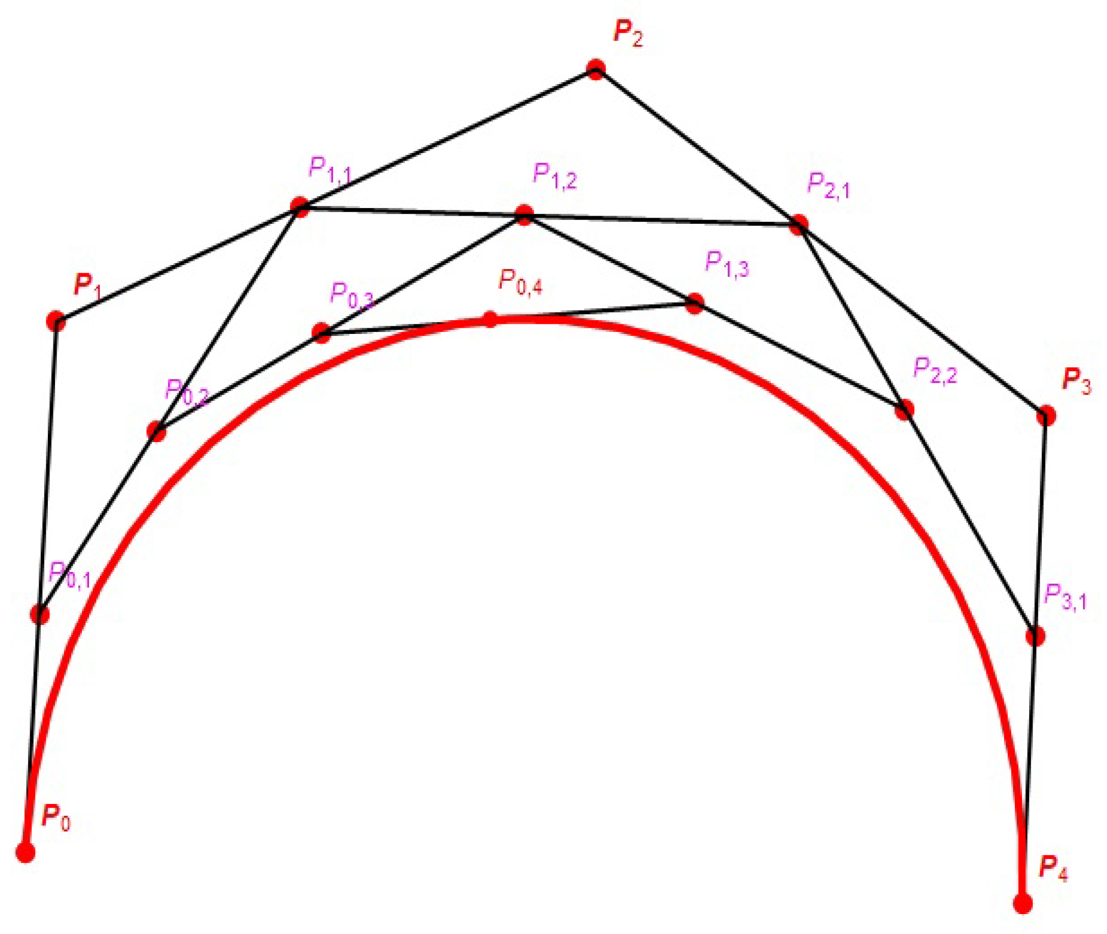
5. Serret-Frenet Elements of Bézier Curve with the Algorithm in E 2 and E 3

For the intermediate points P i , k ( t ) obtained by the control points b 0 , b 1 , . . . , b n (Figure 1) we have the following equation:
P i , k ( t ) = j = 0 k B j , k ( t ) b i + j .
It is obvious that P i , 0 ( t ) = b i and
P 0 , n ( t ) = P ( t ) .
And so, using (20) we obtain n-th degree algorithmic Bézier curve Bézier curve with n + 1 control points by (1). For the intermediate points P i , k ( t ) , we write below recursive formula:
P i , k ( t ) = ( 1 t ) P i , k 1 ( t ) + t P i + 1 , k 1 ( t ) .
Corollary 4.
The subtraction of two intermediate points P i + 1 , k ( t ) and P i , k ( t ) is
P i + 1 , k ( t ) P i , k ( t ) = ( 1 t ) P i + 1 , k 1 ( t ) P i , k 1 ( t ) + t P i + 2 , k 1 ( t ) P i + 1 , k 1 ( t ) .
Proof of Corollary 4.
If we consider (22) for the intermediate point P i + 1 , k ( t ) , we find
P i + 1 , k ( t ) = ( 1 t ) P i + 1 , k 1 ( t ) + t P i + 2 , k 1 ( t ) .
Moreover, by (22), we obtain
P i + 1 , k ( t ) P i , k ( t ) = ( 1 t ) P i + 1 , k 1 ( t ) + t P i + 2 , k 1 ( t ) { ( 1 t ) P i , k 1 ( t ) + t P i + 1 , k 1 ( t ) } = ( 1 t ) P i + 1 , k 1 ( t ) P i , k 1 ( t ) + t P i + 2 , k 1 ( t ) P i + 1 , k 1 ( t ) .
Lemma 1.
The first derivative of n-th degree algorithmic Bézier curve with n + 1 control points given by (21) is
P 0 , n ( t ) = P ( t ) = n P 1 , n 1 ( t ) P 0 , n 1 ( t ) .
Proof of Lemma 1.
We know that the first derivative of algorithmic Bézier curve P ( t ) is given by (4). If we use that equation, we can obtain the following equality:
P ( t ) = n i = 0 n 1 B i , n 1 ( t ) Δ b i = n i = 0 n 1 B i , n 1 ( t ) ( b i + 1 b i ) .
After making the necessary adjustments, we get the following equation:
P ( t ) = n ( i = 0 n 1 B i , n 1 ( t ) b i + 1 i = 0 n 1 B i , n 1 ( t ) b i ) .
Finally, using (20), we obtain the desired equality. □
Corollary 5.
From (23) and (24), we have following two equivalent equalities for the first derivative P 0 , n ( t ) :
P 0 , n ( t ) = n { ( 1 t ) P 1 , n 2 ( t ) P 0 , n 2 ( t ) + t P 2 , n 2 ( t ) P 1 , n 2 ( t ) }
P 0 , n ( t ) = n { ( 1 t ) 2 P 1 , n 3 ( t ) P 0 , n 3 ( t ) + 2 ( 1 t ) t ( P 2 , n 3 ( t ) P 1 , n 3 ( t ) ) + t 2 ( P 3 , n 3 ( t ) P 2 , n 3 ( t ) ) } .
Corollary 6.
An equivalent formulation for the Bézier curve P i , k ( t ) with the control points b i , . . . , b i + k is
P i , k ( t ) = k P i + 1 , k 1 ( t ) P i , k 1 ( t )
where k { 1 , . . . , n } and i { 0 , . . . , n k } .
Lemma 2.
The second derivative of n-th degree algorithmic Bézier curve with n + 1 control points described by (21) is
P 0 , n ( t ) = n ( n 1 ) [ ( P 1 , n 2 ( t ) P 0 , n 2 ( t ) ) ( P 1 , n 2 ( t ) P 0 , n 2 ( t ) ) ] .
Proof of Lemma 2.
The second derivative P 0 , n ( t ) is calculated through (24) and (27) as follows:
( P 0 , n ( t ) ) = ( n P 1 , n 1 ( t ) P 0 , n 1 ( t ) ) = n ( P 1 , n 1 ( t ) P 0 , n 1 ( t ) ) = n ( n 1 ) P 2 , n 2 ( t ) P 1 , n 2 ( t ) ( n 1 ) P 1 , n 2 ( t ) P 0 , n 2 ( t ) = n ( n 1 ) [ ( P 1 , n 2 ( t ) P 0 , n 2 ( t ) ) ( P 1 , n 2 ( t ) P 0 , n 2 ( t ) ) ] .
Corollary 7.
From (23) and (28), we have the following equality:
P 0 , n ( t ) = n ( n 1 ) { ( 1 t ) [ ( P 2 , n 3 ( t ) P 1 , n 3 ( t ) ) ( P 1 , n 3 ( t ) P 0 , n 3 ( t ) ) ] + t [ ( P 3 , n 3 ( t ) P 2 , n 3 ( t ) ) ( P 2 , n 3 ( t ) P 1 , n 3 ( t ) ) ] } .
Lemma 3.
The third derivative of n-th degree algorithmic Bézier curve with n + 1 control points given by (21) is
P 0 , n ( t ) = P ( t ) = n ( n 1 ) ( n 2 ) [ ( P 3 , n 3 ( t ) P 2 , n 3 ( t ) ) 2 ( P 2 , n 3 ( t ) P 1 , n 3 ( t ) ) + ( P 1 , n 3 ( t ) P 0 , n 3 ( t ) ) ] .
Proof of Lemma 3.
We get considering (27) and (28)
P 0 , n ( t ) = P ( t ) = { n ( n 1 ) [ ( P 1 , n 2 ( t ) P 0 , n 2 ( t ) ) ( P 1 , n 2 ( t ) P 0 , n 2 ( t ) ) ] } = n ( n 1 ) [ ( P 1 , n 2 ( t ) P 0 , n 2 ( t ) ) ( P 1 , n 2 ( t ) P 0 , n 2 ( t ) ) ] = n ( n 1 ) ( n 2 ) [ ( P 3 , n 3 ( t ) P 2 , n 3 ( t ) ) 2 ( P 2 , n 3 ( t ) P 1 , n 3 ( t ) ) + ( P 1 , n 3 ( t ) P 0 , n 3 ( t ) ) ] .
Lemma 4.
The cross-product of the vectors P ( t ) and P ( t ) is
P ( t ) × P ( t ) = n 2 ( n 1 ) { ( P 1 , n 2 P 0 , n 2 ) × ( P 2 , n 2 P 1 , n 2 ) } .
Proof of Lemma 4.
By (25) and (28), we have
P ( t ) × P ( t ) = n { ( 1 t ) P 1 , n 2 ( t ) P 0 , n 2 ( t ) + t P 2 , n 2 ( t ) P 1 , n 2 ( t ) } × { n ( n 1 ) [ ( P 1 , n 2 ( t ) P 0 , n 2 ( t ) ) ( P 1 , n 2 ( t ) P 0 , n 2 ( t ) ) ] } = n 2 ( n 1 ) { ( P 1 , n 2 P 0 , n 2 ) × ( P 2 , n 2 P 1 , n 2 ) } .
Corollary 8.
By considering the Corollary 4, the cross-product formula is rewritten as follows:
P ( t ) × P ( t ) = n 2 ( n 1 ) { ( P 1 , n 2 P 0 , n 2 ) × ( P 2 , n 2 P 1 , n 2 ) } = n 2 ( n 1 ) { ( 1 t ) P 1 , n 3 ( t ) P 0 , n 3 ( t ) + t P 2 , n 3 ( t ) P 1 , n 3 ( t ) × ( 1 t ) P 2 , n 3 ( t ) P 1 , n 3 ( t ) + t P 3 , n 3 ( t ) P 2 , n 3 ( t ) } = n 2 ( n 1 ) { ( 1 t ) 2 [ P 1 , n 3 ( t ) P 0 , n 3 ( t ) × P 2 , n 3 ( t ) P 1 , n 3 ( t ) ] + ( 1 t ) t [ P 1 , n 3 ( t ) P 0 , n 3 ( t ) × P 3 , n 3 ( t ) P 2 , n 3 ( t ) ] + t 2 [ P 2 , n 3 ( t ) P 1 , n 3 ( t ) × P 3 , n 3 ( t ) P 2 , n 3 ( t ) ] } .
Corollary 9.
Using Lemma 3 and Corollary 8 the following inner product holds:
P t × P t , P t = N P 1 , n 3 P 0 , n 3 × P 2 , n 3 P 1 , n 3 , P 3 , n 3 P 2 , n 3
where N = n 3 n 1 2 n 2 .
Considering the equations up to now, we recalculate Serret-Frenet elements of the Bézier curve in terms of intermediate points in further section.

5.1. Serret-Frenet Elements of Bézier Curve of Degree n with the Algorithm in E 2

Theorem 4.
The Serret-Frenet frame { T , N } and curvature κ of non-unit speed planar n-th degree algorithmic Bézier curve P 0 , n ( t ) = P ( t ) with the control points b 0 , b 1 , , b n are
T ( t ) = P 1 , n 1 ( t ) P 0 , n 1 ( t ) P 1 , n 1 ( t ) P 0 , n 1 ( t ) t R
N ( t ) = J P 1 , n 1 ( t ) P 0 , n 1 ( t ) P 1 , n 1 ( t ) P 0 , n 1 ( t )
κ ( t ) = n 1 n { P 2 , n 2 ( t ) P 1 , n 2 ( t ) , J ( P 1 , n 1 ( t ) P 0 , n 1 ( t ) ) P 1 , n 1 ( t ) P 0 , n 1 ( t ) 3 P 1 , n 2 ( t ) P 0 , n 2 ( t ) , J ( P 1 , n 1 ( t ) P 0 , n 1 ( t ) ) P 1 , n 1 ( t ) P 0 , n 1 ( t ) 3 }
where P i , k ( t ) are intermediate points given by (20).
Proof of Theorem 4.
The Serret-Frenet elements { T , N , κ } can be obtained using (12), (13), (14), (24) and (28). □
Remark 1.
Notice that the Serret-Frenet elements { T , N , κ } calculated in Theorem 2 and in Theorem 4 are the same.

5.2. Serret-Frenet Elements of Bézier Curve of Degree n with the Algorithm in
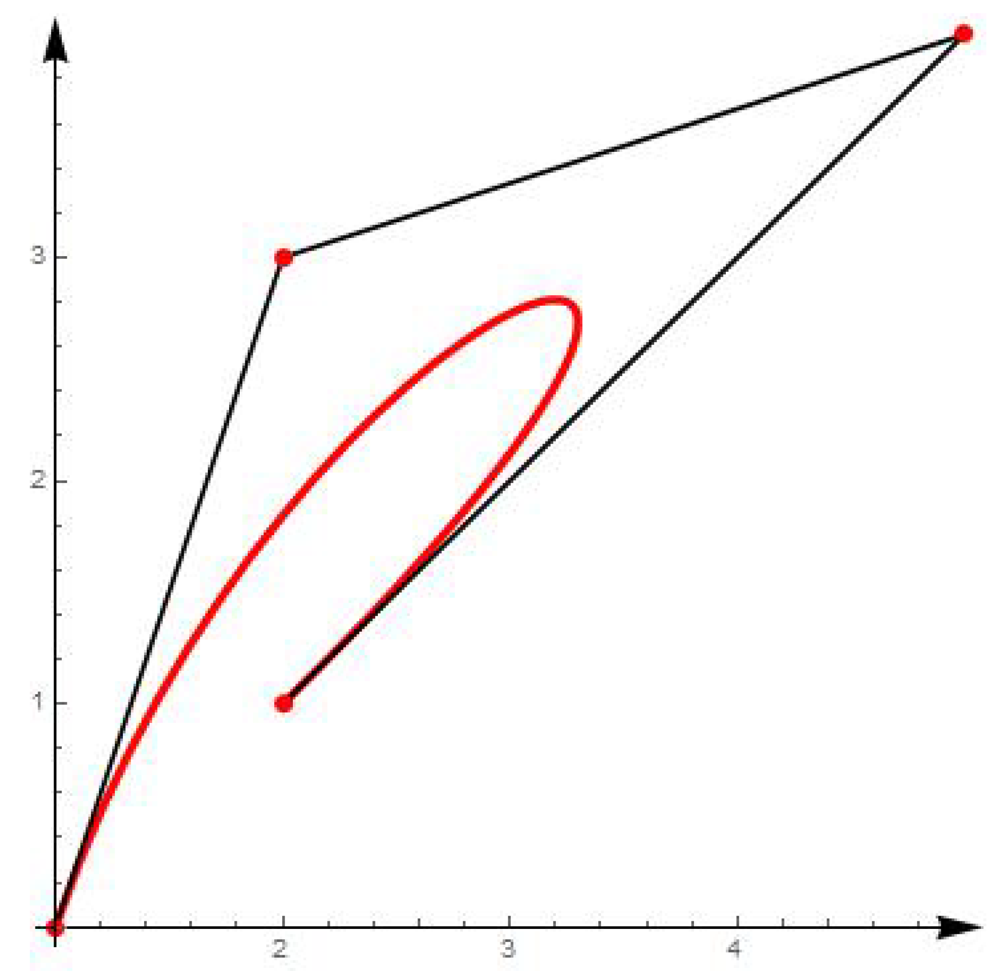
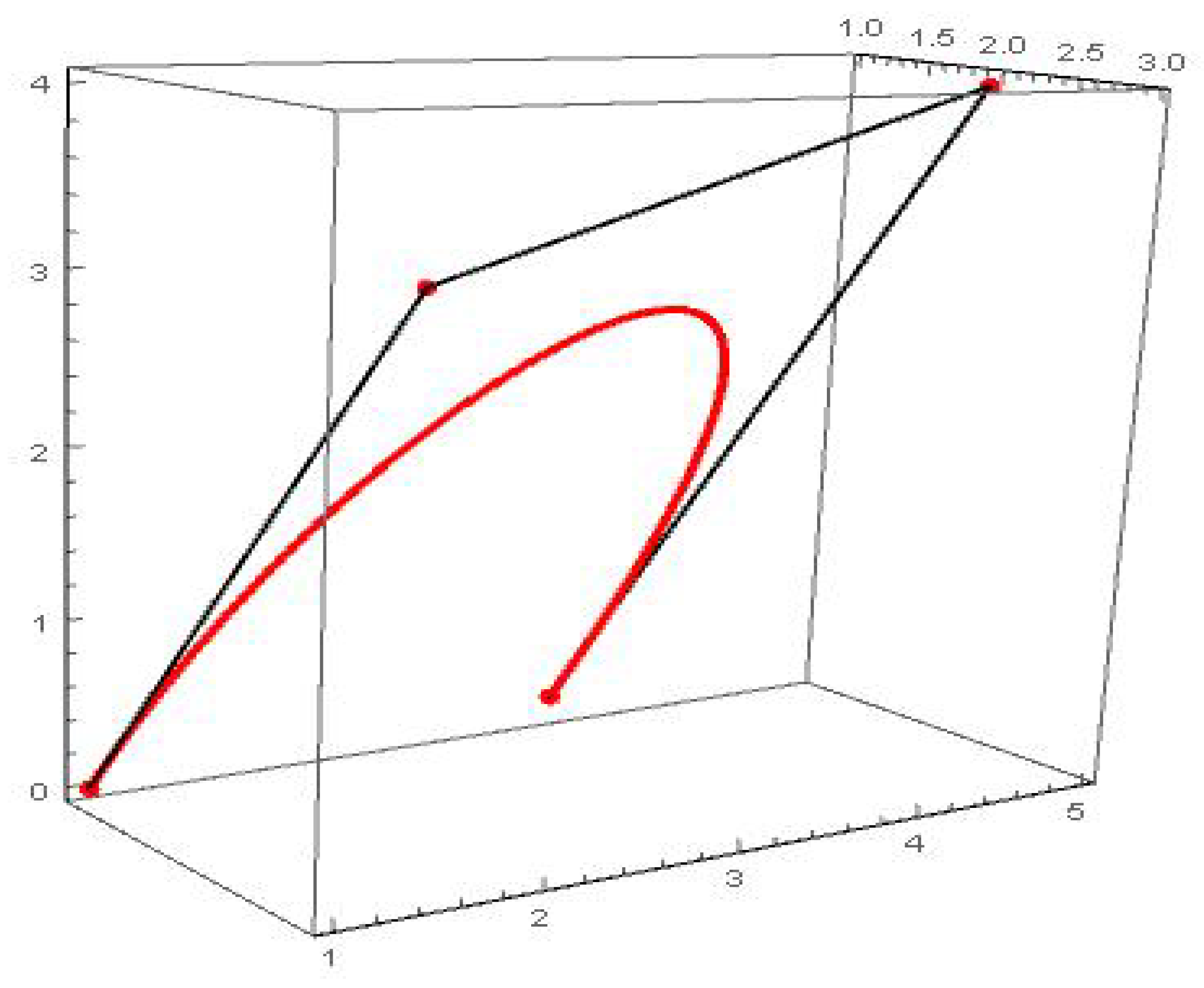
 E 3

Theorem 5.
The Serret-Frenet frame { T , N , B } , curvature κ and torsion τ of non-unit speed spatial n-th degree algorithmic Bézier curve P 0 , n ( t ) = P ( t ) with control points b 0 , b 1 , , b n are
T ( t ) = P 1 , n 1 ( t ) P 0 , n 1 ( t ) P 1 , n 1 ( t ) P 0 , n 1 ( t ) = ( 1 t ) P 1 , n 2 ( t ) P 0 , n 2 ( t ) + t P 2 , n 2 ( t ) P 1 , n 2 ( t ) ( 1 t ) P 1 , n 2 ( t ) P 0 , n 2 ( t ) + t P 2 , n 2 ( t ) P 1 , n 2 ( t ) t R
B ( t ) = ( P 1 , n 2 ( t ) P 0 , n 2 ( t ) ) × ( P 2 , n 2 ( t ) P 1 , n 2 ( t ) ) ( P 1 , n 2 ( t ) P 0 , n 2 ( t ) ) × ( P 2 , n 2 ( t ) P 1 , n 2 ( t ) )
N ( t ) = { ( P 1 , n 2 ( t ) P 0 , n 2 ( t ) ) × ( P 2 , n 2 ( t ) P 1 , n 2 ( t ) ) } × { P 1 , n 1 ( t ) P 0 , n 1 ( t ) } { ( P 1 , n 2 ( t ) P 0 , n 2 ( t ) ) × ( P 2 , n 2 ( t ) P 1 , n 2 ( t ) ) } × { P 1 , n 1 ( t ) P 0 , n 1 ( t ) } = { ( P 1 , n 2 ( t ) P 0 , n 2 ( t ) ) × ( P 2 , n 2 ( t ) P 1 , n 2 ( t ) ) } × { ( 1 t ) P 1 , n 2 ( t ) P 0 , n 2 ( t ) + t P 2 , n 2 ( t ) P 1 , n 2 ( t ) } { ( P 1 , n 2 ( t ) P 0 , n 2 ( t ) ) × ( P 2 , n 2 ( t ) P 1 , n 2 ( t ) ) } × { ( 1 t ) P 1 , n 2 ( t ) P 0 , n 2 ( t ) + t P 2 , n 2 ( t ) P 1 , n 2 ( t ) }
κ ( t ) = n 1 n ( P 1 , n 2 ( t ) P 0 , n 2 ( t ) ) × ( P 2 , n 2 ( t ) P 1 , n 2 ( t ) ) P 1 , n 1 ( t ) P 0 , n 1 ( t ) 3 = n 1 n ( P 1 , n 2 ( t ) P 0 , n 2 ( t ) ) × ( P 2 , n 2 ( t ) P 1 , n 2 ( t ) ) ( 1 t ) ( P 1 , n 2 ( t ) P 0 , n 2 ( t ) ) + t ( P 2 , n 2 ( t ) P 1 , n 2 ( t ) ) 3
τ ( t ) = n 2 n ( P 1 , n 3 ( t ) P 0 , n 3 ( t ) ) × ( P 2 , n 3 ( t ) P 1 , n 3 ( t ) ) , ( P 3 , n 3 ( t ) P 2 , n 3 ( t ) ) ( P 1 , n 2 ( t ) P 0 , n 2 ( t ) ) × ( P 2 , n 2 ( t ) P 1 , n 2 ( t ) ) 2 = n 2 n ( P 1 , n 3 ( t ) P 0 , n 3 ( t ) ) × ( P 2 , n 3 ( t ) P 1 , n 3 ( t ) ) , ( P 3 , n 3 ( t ) P 2 , n 3 ( t ) ) { ( 1 t ) ( P 1 , n 3 ( t ) P 0 , n 3 ( t ) ) + t ( P 2 , n 3 ( t ) P 1 , n 3 ( t ) ) } × { ( 1 t ) ( P 2 , n 3 ( t ) P 1 , n 3 ( t ) ) + t ( P 3 , n 3 ( t ) P 2 , n 3 ( t ) ) } 2
where P i , k ( t ) ’s are intermediate points given by (20).
Proof of Theorem 5.
The desired equalities in Theorem 5 are procured through (15)–(19) and (20)–(33). □
Remark 2.
Notice that the Serret-Frenet elements { T , N , B , κ , τ } in Theorem 3 and in Theorem 5 are the same.

6. Examples in E 2 and E 3

Example 1.
Let consider control points b 0 = ( 1 , 0 ) , b 1 = ( 2 , 3 ) , b 2 = ( 5 , 4 ) and b 3 = ( 2 , 1 ) for cubic Bézier curve in Euclidean plane E 2 (Figure 2). With these control points, the Serret-Frenet frame { T , N } and curvature κ P 3 of cubic Bézier curve are found as in the following steps, respectively, for each t R , t = 0 and t = 1 .
By (3) and definition of Bernstein polynomial, cubic Bézier curve is written as follows:
P 3 ( t ) = B 0 , 3 ( t ) b 0 + B 1 , 3 ( t ) b 1 + B 2 , 3 ( t ) b 2 + B 3 , 3 ( t ) b 3 = ( 1 t ) 3 b 0 + 3 ( 1 t ) 2 t b 1 + 3 ( 1 t ) t 2 b 2 + t 3 b 3 = ( ( 1 t ) 3 + 6 t ( 1 t ) 2 + 15 t 2 ( 1 t ) + 2 t 3 , 9 t ( 1 t ) 2 + 12 t 2 ( 1 t ) + t 3 ) .
  • The Serret-Frenet frame { T , N } and curvature κ P 3 for t R are
    T ( t ) = ( 1 t ) 2 Δ 1 b 0 + 2 ( 1 t ) t Δ 1 b 1 + t 2 Δ 1 b 2 ( 1 t ) 2 Δ 1 b 0 + 2 ( 1 t ) t Δ 1 b 1 + t 2 Δ 1 b 2 = 8 t 2 + 4 t + 1 , 2 t 2 4 t + 3 8 t 2 + 4 t + 1 , 2 t 2 4 t + 3
    N ( t ) = ( 1 t ) 2 J Δ 1 b 0 + 2 ( 1 t ) t J Δ 1 b 1 + t 2 J Δ 1 b 2 ( 1 t ) 2 Δ 1 b 0 + 2 ( 1 t ) t Δ 1 b 1 + t 2 Δ 1 b 2 = 2 t 2 + 4 t 3 , 8 t 2 + 4 t + 1 8 t 2 + 4 t + 1 , 2 t 2 4 t + 3
    κ P 3 ( t ) = 2 3 ( 1 t ) 2 Δ 1 b 1 , J Δ 1 b 0 + ( 1 t ) t Δ 1 b 2 , J Δ 1 b 0 + t 2 Δ 1 b 2 , J Δ 1 b 1 ( 1 t ) 2 Δ 1 b 0 + 2 ( 1 t ) t Δ 1 b 1 + t 2 Δ 1 b 2 3 = 2 3 20 t 2 + 22 t 8 8 t 2 + 4 t + 1 , 2 t 2 4 t + 3 3 .
  • The Serret-Frenet frame { T , N } and curvature κ P 3 for t = 0 are
    T ( t ) t = 0 = Δ 1 b 0 Δ 1 b 0 = 1 10 ( 1 , 3 )
    N ( t ) t = 0 = J Δ 1 b 0 Δ 1 b 0 = 1 10 ( 3 , 1 )
    κ P 3 ( t ) t = 0 = 2 3 Δ 1 b 1 , J Δ 1 b 0 Δ 1 b 0 3 = 2 3 Δ 1 b 1 , J Δ 1 b 0 Δ 1 b 0 , Δ 1 b 0 3 / 2 = 0 .
  • The Serret-Frenet frame { T , N } and curvature κ P 3 for t = 1 are
    T ( t ) t = 1 = Δ 1 b 2 Δ 1 b 2 = 1 3 2 ( 3 , 3 )
    N ( t ) t = 1 = J Δ 1 b 2 Δ 1 b 2 = 1 3 2 ( 3 , 3 )
    κ P 3 ( t ) t = 1 = 2 3 Δ 1 b 2 , J Δ 1 b 1 Δ 1 b 2 3 = 2 27 2 .
Example 2.
Confirm that Theorem 4 holds for cubic Bézier curve given in Example 1.
By (20) and definition of Bernstein polynomial, cubic Bézier curve in Example 1 is given as follows:
P 0 , 3 ( t ) = ( 1 t ) 3 + 6 t ( 1 t ) 2 + 15 t 2 ( 1 t ) + 2 t 3 , 9 t ( 1 t ) 2 + 12 t 2 ( 1 t ) + t 3 .
Writing n = 3 in Theorem 4, we obtain Serret-Frenet elements { T , N , κ } for cubic Bézier curve as folllows:
T ( t ) = P 1 , 2 ( t ) P 0 , 2 ( t ) P 1 , 2 ( t ) P 0 , 2 ( t )
N ( t ) = J P 1 , 2 ( t ) P 0 , 2 ( t ) P 1 , 2 ( t ) P 0 , 2 ( t )
κ ( t ) = 2 3 { P 2 , 1 ( t ) P 1 , 1 ( t ) , J P 1 , 2 ( t ) P 0 , 2 ( t ) P 1 , 2 ( t ) P 0 , 2 ( t ) 3 P 1 , 1 ( t ) P 0 , 1 ( t ) , J P 1 , 2 ( t ) P 0 , 2 ( t ) P 1 , 2 ( t ) P 0 , 2 ( t ) 3 } .
Using (20), we can write the following equations:
P 0 , 2 ( t ) = j = 0 2 B j , 2 ( t ) b j = ( 1 t ) 2 b 0 + 2 t ( 1 t ) b 1 + t 2 b 2 ,
P 1 , 2 ( t ) = j = 0 2 B j , 2 ( t ) b 1 + j = ( 1 t ) 2 b 1 + 2 t ( 1 t ) b 2 + t 2 b 3 ,
P 0 , 1 ( t ) = j = 0 1 B j , 1 ( t ) b j = ( 1 t ) b 0 + t b 1 ,
P 1 , 1 ( t ) = j = 0 1 B j , 1 ( t ) b 1 + j = ( 1 t ) b 1 + t b 2 ,
P 2 , 1 ( t ) = j = 0 1 B j , 1 ( t ) b 2 + j = ( 1 t ) b 2 + t b 3
and
P 1 , 2 ( t ) P 0 , 2 ( t ) = ( 1 t ) 2 Δ b 0 + 2 t ( 1 t ) Δ b 1 + t 2 Δ b 2 , P 1 , 1 ( t ) P 0 , 1 ( t ) = ( 1 t ) Δ b 0 + t Δ b 1 , P 2 , 1 ( t ) P 1 , 1 ( t ) = ( 1 t ) Δ b 1 + t Δ b 2 .
Then, using the above equations, we can obtain the equations in Example 1.
Example 3.
Consider the control points b 0 = ( 1 , 0 , 1 ) , b 1 = ( 2 , 3 , 2 ) , b 2 = ( 5 , 4 , 2 ) and b 3 = ( 2 , 1 , 3 ) for cubic Bézier curve (Figure 3).
We check that the results of Theorem 3 and Theorem 5 are same by using above cubic Bézier curve.
By (20) and definition of Bernstein polynomial, the cubic Bézier curve for this example is
P 0 , 3 ( t ) = ( ( 1 t ) 3 + 6 t ( 1 t ) 2 + 15 t 2 ( 1 t ) + 2 t 3 , 9 t ( 1 t ) 2 + 12 t 2 ( 1 t ) + t 3 , ( 1 t ) 3 + 6 t ( 1 t ) 2 + 6 t 2 ( 1 t ) + 3 t 3 )
  • By taking n = 3 in Theorem 5, we obtain Serret-Frenet elements { T , N , B , κ , τ } for cubic Bézier curve as follows:
    T ( t ) = P 1 , 2 ( t ) P 0 , 2 ( t ) P 1 , 2 ( t ) P 0 , 2 ( t )
    B ( t ) = ( P 1 , 1 ( t ) P 0 , 1 ( t ) ) × ( P 2 , 1 ( t ) P 1 , 1 ( t ) ) ( P 1 , 1 ( t ) P 0 , 1 ( t ) ) × ( P 2 , 1 ( t ) P 1 , 1 ( t ) )
    N ( t ) = { ( P 1 , 1 ( t ) P 0 , 1 ( t ) ) × ( P 2 , 1 ( t ) P 1 , 1 ( t ) ) } × { P 1 , 2 ( t ) P 0 , 2 ( t ) } { ( P 1 , 1 ( t ) P 0 , 1 ( t ) ) × ( P 2 , 1 ( t ) P 1 , 1 ( t ) ) } × { P 1 , 2 ( t ) P 0 , 2 ( t ) }
    κ ( t ) = 2 3 ( P 1 , 1 ( t ) P 0 , 1 ( t ) ) × ( P 2 , 1 ( t ) P 1 , 1 ( t ) ) P 1 , 2 ( t ) P 0 , 2 ( t ) 3
    τ ( t ) = 1 3 ( P 1 , 0 ( t ) P 0 , 0 ( t ) ) × ( P 2 , 0 ( t ) P 1 , 0 ( t ) ) , ( P 3 , 0 ( t ) P 2 , 0 ( t ) ) ( P 1 , 1 ( t ) P 0 , 1 ( t ) ) × ( P 2 , 1 ( t ) P 1 , 1 ( t ) ) 2 .
Using (20), we can write the following equations:
P 1 , 2 ( t ) P 0 , 2 ( t ) = ( 1 t ) 2 Δ 1 b 0 + 2 t ( 1 t ) Δ 1 b 1 + t 2 Δ 1 b 2 P 1 , 1 ( t ) P 0 , 1 ( t ) = ( 1 t ) Δ 1 b 0 + t Δ 1 b 1 P 2 , 1 ( t ) P 1 , 1 ( t ) = ( 1 t ) Δ 1 b 1 + t Δ 1 b 2 P 3 , 0 ( t ) P 2 , 0 ( t ) = b 3 b 2 = Δ 1 b 2 P 2 , 0 ( t ) P 1 , 0 ( t ) = b 2 b 1 = Δ 1 b 1 P 1 , 0 ( t ) P 0 , 0 ( t ) = b 1 b 0 = Δ 1 b 0
.
Therefore, we have
T ( t ) = ( 1 t ) 2 Δ 1 b 0 + 2 t ( 1 t ) Δ 1 b 1 + t 2 Δ 1 b 2 ( 1 t ) 2 Δ 1 b 0 + 2 t ( 1 t ) Δ 1 b 1 + t 2 Δ 1 b 2 = ( 8 t 2 + 4 t + 1 , 2 t 2 4 t + 3 , 1 2 t + 2 t 2 ) ( 8 t 2 + 4 t + 1 , 2 t 2 4 t + 3 , 1 2 t + 2 t 2 )
B ( t ) = ( 1 t ) 2 ( Δ 1 b 0 × Δ 1 b 1 ) + t ( 1 t ) ( Δ 1 b 0 × Δ 1 b 2 ) + t 2 ( Δ 1 b 1 × Δ 1 b 2 ) ( 1 t ) 2 ( Δ 1 b 0 × Δ 1 b 1 ) + t ( 1 t ) ( Δ 1 b 0 × Δ 1 b 2 ) + t 2 ( Δ 1 b 1 × Δ 1 b 2 ) = ( 6 t 2 + 8 t 1 , 4 t 2 10 t + 3 , 20 t 2 + 22 t 8 ) ( 6 t 2 + 8 t 1 , 4 t 2 10 t + 3 , 20 t 2 + 22 t 8 )
N ( t ) = B ( t ) × T ( t ) = ( 32 t 4 + 64 t 3 142 t 2 + 114 t 27 , 172 t 4 284 t 3 + 156 t 2 20 t 7 , 20 t 4 72 t 3 + 36 t 2 28 t + 6 ) ( 8 t 2 + 4 t + 1 , 2 t 2 4 t + 3 , 1 2 t + 2 t 2 ) ( 6 t 2 + 8 t 1 , 4 t 2 10 t + 3 , 20 t 2 + 22 t 8 )
κ ( t ) = 2 3 ( 6 t 2 + 8 t 1 , 4 t 2 10 t + 3 , 20 t 2 + 22 t 8 ) ( 8 t 2 + 4 t + 1 , 2 t 2 4 t + 3 , 1 2 t + 2 t 2 ) 3
and
τ ( t ) = 1 3 Δ 1 b 0 × Δ 1 b 1 , Δ 1 b 2 ( 6 t 2 + 8 t 1 , 4 t 2 10 t + 3 , 20 t 2 + 22 t 8 ) 2 = 1 3 14 ( 6 t 2 + 8 t 1 , 4 t 2 10 t + 3 , 20 t 2 + 22 t 8 ) 2 .
  • By taking n = 3 in Theorem 3, we obtain Serret-Frenet elements { T , N , B , κ , τ } for cubic Bézier curve as follows:
    T ( t ) = i = 0 2 B i , 2 ( t ) Δ 1 b i i = 0 2 B i , 2 ( t ) Δ 1 b i
    B ( t ) = i = 0 2 j = 0 1 B i , 2 ( t ) B j , 1 ( t ) ( Δ 1 b i × Δ 2 b j ) i = 0 2 j = 0 1 B i , 2 ( t ) B j , 1 ( t ) ( Δ 1 b i × Δ 2 b j )
    N ( t ) = i = 0 2 j = 0 1 k = 0 2 B i , 2 ( t ) B j , 1 ( t ) B k , 2 ( t ) ( Δ 1 b i × Δ 2 b j ) × Δ b k i = 0 2 j = 0 1 k = 0 2 B i , 2 ( t ) B j , 1 ( t ) B k , 2 ( t ) ( Δ 1 b i × Δ 2 b j ) × Δ b k
    κ ( t ) = 2 3 i = 0 2 j = 0 1 B i , 2 ( t ) B j , 1 ( t ) ( Δ 1 b i × Δ 2 b j ) i = 0 2 B i , 2 ( t ) Δ 1 b i 3
    τ ( t ) = 1 3 i = 0 2 j = 0 1 k = 0 0 B i , 2 ( t ) B j , 1 ( t ) B k , 0 ( t ) Δ 1 b i × Δ 2 b j , Δ 3 b k i = 0 2 j = 0 1 B i , 2 ( t ) B j , 1 ( t ) ( Δ 1 b i × Δ 2 b j ) 2 .
Using (1), we write the following two equalities:
i = 0 2 B i , 2 ( t ) Δ 1 b i = ( 1 t ) 2 Δ 1 b 0 + 2 t ( 1 t ) Δ 1 b 1 + t 2 Δ 1 b 2 = ( 8 t 2 + 4 t + 1 , 2 t 2 4 t + 3 , 1 2 t + 2 t 2 )
and
i = 0 2 j = 0 1 B i , 2 ( t ) B j , 1 ( t ) ( Δ 1 b i × Δ 2 b j ) = ( 1 2 t + t 2 ) ( Δ 1 b 0 × Δ 1 b 1 ) + ( t t 2 ) ( Δ 1 b 0 × Δ 1 b 2 ) + t 2 ( Δ 1 b 1 × Δ 1 b 2 ) = ( 6 t 2 + 8 t 1 , 4 t 2 10 t + 3 , 20 t 2 + 22 t 8 ) .
After all, we have
T ( t ) = ( 8 t 2 + 4 t + 1 , 2 t 2 4 t + 3 , 1 2 t + 2 t 2 ) ( 8 t 2 + 4 t + 1 , 2 t 2 4 t + 3 , 1 2 t + 2 t 2 )
B ( t ) = ( 6 t 2 + 8 t 1 , 4 t 2 10 t + 3 , 20 t 2 + 22 t 8 ) ( 6 t 2 + 8 t 1 , 4 t 2 10 t + 3 , 20 t 2 + 22 t 8 )
N ( t ) = B ( t ) × T ( t )
= ( 32 t 4 + 64 t 3 142 t 2 + 114 t 27 , 172 t 4 284 t 3 + 156 t 2 20 t 7 , 20 t 4 72 t 3 + 36 t 2 28 t + 6 ) ( 8 t 2 + 4 t + 1 , 2 t 2 4 t + 3 , 1 2 t + 2 t 2 ) ( 6 t 2 + 8 t 1 , 4 t 2 10 t + 3 , 20 t 2 + 22 t 8 )
κ ( t ) = 2 3 ( 6 t 2 + 8 t 1 , 4 t 2 10 t + 3 , 20 t 2 + 22 t 8 ) ( 8 t 2 + 4 t + 1 , 2 t 2 4 t + 3 , 1 2 t + 2 t 2 ) 3
and
τ ( t ) = 1 3 i = 0 2 j = 0 1 k = 0 0 B i , 2 ( t ) B j , 1 ( t ) B k , 0 ( t ) Δ 1 b i × Δ 2 b j , Δ 3 b k i = 0 2 j = 0 1 B i , 2 ( t ) B j , 1 ( t ) ( Δ 1 b i × Δ 2 b j ) 2 = 1 3 14 ( 6 t 2 + 8 t 1 , 4 t 2 10 t + 3 , 20 t 2 + 22 t 8 ) 2 .

7. Conclusions

Bézier curves are mostly used in the field of Computer Aided Design and advantageous in terms of design. In this study, we have discussed these curves with regard to differential geometry. We examined the Serret-Frenet elements, which are the essential elements of the curve, for the Bézier curve in Euclidean plane E 2 and Euclidean space E 3 . These elements have been studied in the literature only at end points for spatial Bézier curves. For these curves, we have calculated these elements at the end points and for each parameter t in Euclidean plane E 2 . Additionally, we have calculated these elements at the end points and for each parameter t in Euclidean space E 3 .
In addition, we have discussed these elements again, giving the definition of the algorithmic Bézier curve in Euclidean plane E 2 and Euclidean space E 3 for each parameter t. In the calculations made without the algorithm, the derivative calculation is less stable and more time-consuming. Stability and time are important in curve and surface designing. As a result, the calculations using algorithm have more advantageous.

Author Contributions

S.Y. suggested an idea of handling the Bézier curves in terms of differential geometry, based on the missing parts in the literature; E.E. constructed the theory of this idea; both co-wrote the paper.

Funding

This research received no external funding.

Acknowledgments

Esra Erkan gratefully acknowledged The Scientific and Technological Research Council of Turkey (TÜBİTAK) for its partially support for this study.

Conflicts of Interest

The authors declare no conflicts of interest.

References

  1. Anand, V.B. Computer Graphics and Geometric Modeling for Engineers, 1st ed.; John Wiley and Sons Inc.: New York, NY, USA, 1992. [Google Scholar]
  2. Iglesias, A.; Gálvez, A.; Loucera, C. Two Simulated Annealing Optimization Schemas for Rational Bézier Curve Fitting in the Presence of Noise. Math. Prob. Eng. 2016, 2016, 8241275. [Google Scholar] [CrossRef]
  3. Forrest, A.R. Curves and Surfaces for Computer-Aided Design. Ph.D. Thesis, University of Cambridge, Cambridge, UK, 1968. [Google Scholar]
  4. Farin, G. Curves and Surfaces for Computer Aided Geometric Design a Practical Guide, 4th ed.; Academic Press: San Diego, CA, USA, 1996. [Google Scholar]
  5. Ghomanjani, F.; Farahi, M.H.; Kılıçman, A.; Kamyad, A.V.; Pariz, N. Bézier Curves Based Numerical Solutions of Delay Systems with Inverse Time. Math. Prob. Eng. 2014. [Google Scholar] [CrossRef]
  6. Hu, G.; Cao, H.; Zhang, S. Approximate Multidegree Reduction of λ-Bézier Curves. Math. Prob. Eng. 2016. [Google Scholar] [CrossRef]
  7. Hu, G.; Ji, X.; Qin, X.; Zhang, S. Shape Modification for λ-Bézier Curves Based on Constrained Optimization of Position and Tangent Vector. Math. Prob. Eng. 2015, 12, 735629. [Google Scholar] [CrossRef]
  8. Misro, M.Y.; Ramli, A.; Ali, J.M. Quintic Trigonometric Bézier Curve with Two Shape Parameters. Sains Malays. 2017, 46, 825–831. [Google Scholar]
  9. Farin, G.; Sapidis, N. Curvature and the fairness of Curves and Surfaces. IEEE Comput. Gr. Appl. 1989, 9, 52–57. [Google Scholar] [CrossRef]
  10. Frey, W.H.; Field, D.A. Designing Bézier Conic Segments with Monotone Curvature. Comput. Aided Geom. Des. 2000, 17, 457–483. [Google Scholar] [CrossRef]
  11. Goldman, R. Curvature Formulas for Implicit Curves and Surfaces. Comput. Aided Geom. Des. 2005, 22, 632–658. [Google Scholar] [CrossRef]
  12. Farin, G.; Hoschek, J.; Kim, M.S. Handbook of Computer Aided Geometric Design; Elsevier Science: Amsterdam, The Netherlands, 2002. [Google Scholar]
  13. Marsh, D. Applied Geometry for Computer Graphics and CAD, 2nd ed.; Springer: London, UK; Berlin/Heidelberg, Germany, 2004. [Google Scholar]
  14. Kusak Samanci, H.; Celik, S.; Incesu, M. The Bishop Frame of Bézier Curves. Life Sci. J. 2015, 12, 175–180. [Google Scholar]
  15. Gray, A.; Abbena, E.; Salamon, S. Modern Differential Geometry of Curves and Surfaces with Mathematica; Chapman and Hall/CRC: Boca Raton, FL, USA, 2016. [Google Scholar]
Figure 1. Intermediate points for i = 0 and n = 4 .
Mathematics 06 00321 g001
Figure 2. Cubic Bézier curve in E 2 .
Mathematics 06 00321 g002
Figure 3. Cubic Bézier curve in E 3 .
Mathematics 06 00321 g003

