1. Introduction
The Riemann hypothesis continues to defeat all attempts to prove or disprove it [
1,
2,
3,
4,
5,
6]. On the other hand assuming the Riemann hypothesis provides a wealth of intriguing tentative suggestions regarding the distribution of the prime numbers [
1,
2,
3,
4,
5,
6]. However, even the Riemann hypothesis is insufficient to prove Andrica’s conjecture [
7,
8,
9]:
(In
Section 6 below, by considering the known maximal prime gaps, I shall numerically [and unconditionally] verify Andrica’s conjecture up to just below the 81
st maximal prime gap; certainly for all primes less than
.) Somewhat weaker results that have been unconditionally proved include Sandor’s 1985 result [
10]
and the more recent 2017 result by Lowry–Duda [
11] that for
,
, and
:
Other recent articles on the distribution of primes include [
12,
13].
In the current article I shall seek to derive results as close to Andrica’s conjecture as possible. The basic tools we use are based on the behaviour of prime gaps under the Riemann hypothesis. I shall primarily make use of the recent fully explicit bound due to Carneiro, Milinovich, and Soundararajan [
14]:
Theorem 1 (Prime gaps; Carneiro–Milinovich–Soundararajan)
. Assuming the Riemann hypothesis,
(In
Section 7 below, by considering the known maximal prime gaps, I shall numerically [and unconditionally] verify this result up to just below the 81
st maximal prime gap; certainly for all primes less than
.) The “close to Andrica” results I will prove below are these:
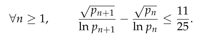
Theorem 2 (Logarithmic modification of Andrica)
. Assuming the Riemann hypothesis, Theorem 3 (Higher root modification of Andrica)
. Assuming the Riemann hypothesis, 2. Known Results on Prime Gaps Assuming Riemann Hypothesis
Two older theorems addressing the issue of prime gaps are “ineffective” (meaning one or more implicit constants are known to be finite but are otherwise undetermined):
Theorem 4 (Cramer 1919 [
15,
16])
. Assuming the Riemann hypothesis, Unfortunately, this particular theorem only gives qualitative, but not quantitative, information.
Theorem 5 (Goldston 1982 [
17])
. Assuming the Riemann hypothesis, This particular theorem gives quantitative information about the size of prime gaps, but only qualitative information as to the domain of validity. The considerably more recent Carneiro, Milinovich, and Soundararajan theorem [
14], presented as Theorem 1 above, is fully explicit. It is that theorem that will be my primary tool.
3. Logarithmic Modification of Andrica: Proof of Theorem 2
The proof of Theorem 2, given our input assumptions, is straightforward.
Consider the function
and note
So
is certainly monotone and convex for
. Thence for
, that is
, we have
(The first step in this chain of inequalities is based on convexity, the second step on the Carneiro–Milinovich–Soundararajan result; the remaining steps are trivial.) A quick verification shows that this inequality also holds for
and so we have
This by no means an optimal bound, but it is, given the Riemann hypothesis and the Carneiro–Milinovich–Soundararajan prime gap result it implies, both easy to establish and easy to work with.
4. Higher-Root Modification Of Andrica: Proof of Theorem 3
The proof of Theorem 3, given our input assumptions, is straightforward.
Consider the function
and restrict attention to
and
. Then
Thus the function
is monotone and convex for
and
. We have
(The first step in this chain of inequalities is based on convexity, the second step on the Carneiro–Milinovich–Soundararajan result.) If
this result is true but not particularly interesting. For
the function
rises from zero (at
) to a maximum, and subsequently dies back to zero asymptotically as
. The maximum occurs at
where the function takes on the value
, thereby implying
This is the result we were seeking to establish. This is again by no means an optimal bound, but it is, given the Riemann hypothesis and the Carneiro–Milinovich–Soundararajan prime gap result it implies, both easy to establish and easy to work with.
Note that for
, the situation relevant to the standard Andrica conjecture, we merely have
For this is not enough to conclude anything useful regarding the standard Andrica conjecture.
In contrast for
and
we certainly have:
Corollary 1 (Cube root modification of Andrica)
. Assuming the Riemann hypothesis, Corollary 2 (Fourth root modification of Andrica)
. Assuming the Riemann hypothesis, 5. Unconditional Results for Andrica–Like Variants
I shall now focus on some much weaker but unconditional results. A number of explicit unconditional theorems on the occurrence of primes in small gaps are of the following general form.
Theorem 6 (Primes in short intervals)
. For , , and some explicit , there is always at least one prime in the interval:Specifically, we have: | | | Reference | arXiv |
| 396738 | 2 | | Dusart 2010 [18] | 1002.0442 |
| 2898329 | 2 | | Trudgian 2014 [19] | 1401.2689 |
| 468991632 | 2 | | Dusart 2018 [20] | — |
| 89693 | 3 | 1 | Dusart 2018 [20] | — |
| 6034256 | 3 | 0.087 | Axler 2017 [21] | 1703.08032 |
| 1 | 4 | 198.2 | Axler 2017 [21] | 1703.08032 |
Taking
in Theorem 6, this becomes a bound on the prime gaps.
Theorem 7 (Prime gaps)
. For , that is , and taking and from Theorem 6, the prime gaps are unconditionally bounded by: Now consider the function
and note
Then, in view of the convexity of
on the specified domain, we have
That is, we have demonstrated:
Theorem 8 (Explicit unconditional bounds)
. For , that is, , and taking and from the table in Theorem 6, we have the explicit unconditional bounds: While weak, these bounds are both unconditional and fully explicit. I shall now explore several corollaries.
Proof. The general result above already implies this for , that is , the remaining cases can be checked by explicit calculation. □
This bound, for the specified value 0.348, is sharp—it fails by 5% for , .
I shall now present a more relaxed bound with a wider range of validity.
Proof. Use the previous corollary for and check by explicit calculation. □
This bound, for the specified value
, is sharp—it fails by over 50% for
,
. I now present a more relaxed bound with a wider range of validity.
This bound, for the specified value
, is sharp—it fails by over 57% for
,
. I now present an even more relaxed bound with a wider range of validity.
Proof. Use the previous corollary for and check by explicit calculation. □
While all relatively weak, all these bounds have the pronounced virtue of being both fully explicit, and completely unconditional. Furthermore is is now clear how to systematically turn prime gap results of the type considered in Theorem 6 into Andrica-like bounds of the type considered in Theorem 8.
6. Unconditional Numerical Results for the Standard Andrica Conjecture
Andrica’s conjecture can be rearranged to be equivalent to
In an unpublished note (see comments in References [
8,
9]) Imran Ghory rephrased this in terms of maximal prime gaps. Let the triplet
denote the
maximal prime gap; of width
, starting at the prime
. (See see the sequences A005250, A002386, A005669, A000101, A107578.) 80 such maximal prime gaps are currently known [
22], up to
and
. Imran Ghory observed the equivalent of
That is, Andrica’s conjecture certainly holds on the interval
if one has
But this is easily checked to hold on the intervals , , , , , , , and . Thus Andrica’s conjecture certainly holds up to the 80th maximal prime gap, . This bound will certainly be improved as additional maximal prime gaps are identified.
As a slight variant on this argument, consider the interval
, from the lower end of the
maximal prime gap to just below the beginning of the
maximal prime gap. Then everywhere in this interval
That is, Andrica’s conjecture certainly holds on the entire interval if it holds at the beginning of this interval.
Consequently, explicitly checking the inequality for , Andrica’s conjecture holds unconditionally up to just before the beginning of the 81st maximal prime gap, , even if we do not yet know the value of .
7. Unconditional Numerical Results for the Carneiro–Milinovich–Soundararajan Inequality
Consider the Carneiro–Milinovich–Soundararajan inequality
and note that the right-hand side is monotone increasing. Again consider the interval
, from the lower end of the
maximal prime gap to just below the beginning of the
maximal prime gap. Then the Carneiro–Milinovich–Soundararajan inequality certainly holds on the entire interval
if it holds at the beginning of this interval. Explicitly checking the inequality for all the known maximal prime gaps up to
, see reference [
22], the Carneiro–Milinovich–Soundararajan inequality holds unconditionally up to just before the beginning of the 81
st maximal prime gap,
, even if we do not yet know the value of
. Certainly the the Carneiro–Milinovich–Soundararajan inequality holds for all primes less than
. (Of course, assuming the Riemann hypothesis, Carneiro–Milinovich–Soundararajan have theorem; so this numerical exercise is only a partial numerical check on the input to our arguments.) This also implies that theorems 2 and 3 are unconditionally numerically verified for all primes less than
.
8. Discussion
While the Riemann hypothesis provides (among very many other things) a nice explicit bound on prime gaps, it is still not quite sufficient to prove Andrica’s conjecture—though as seen above, one can get tolerably close. There are a number of places where the argument might be tightened—the presentation above was designed to be simple and direct, not necessarily optimal. Of course the really big improvement in theorems 1–2–3 would be if any of these results could be made unconditional. While the numerical evidence certainly suggests this, a proof seems impossible with current techniques.
In contrast what we can currently prove unconditionally is rather weak; so improving the constants in theorems 6–7–8 would also be of some considerable interest.


