Error Bound for Non-Zero Initial Condition Using the Singular Perturbation Approximation Method

Abstract

In this article, we present up to date results on the balanced model reduction techniques for linear control systems, in particular the singular perturbation approximation. One of the most important features of this method is it allows for an a priori $L^2$ and $H^{\infty }$ bounds for the approximation error. This method has been successfully applied for systems with homogeneous initial conditions, however, the main focus in this work is to derive an $L^2$ error bound for singular perturbation approximation for system with inhomogeneous initial conditions, extending the work by Antoulas et al. The theoretical results are validated numerically.

1. Introduction

Linear systems have been under investigation for quite long time due to their wide range of applications in physics, mathematics and engineering. However, the subject is such a fundamental and deep one that there is no doubt that linear systems will continue to be a main focus of study for long time to come.

The modeling of many physical, chemical or biological phenomena resulting from discretized partial differential equations lead to the well-known representation of a linear time-invariant (LTI) system

$$\begin{array}{c}\hfill \begin{array}{cc}\hfill \dot{x}& =Ax+Bu\hfill \\ \hfill y& =Cx+Du\hfill \\ \hfill x(t_0)& =x_0\hfill \end{array}\end{array}$$

(1)

where $A\in {\Re }^{n\times n}$, $B\in {\Re }^{n\times m}$, $C\in {\Re }^{p\times n}$ and $D^{p\times m}$ are constant matrices.

The order n of the system ranges from a few tens to several hundreds as in control problems for large flexible space structures. A common feature of the model used is that it is high-dimensional and displays a variety of time scales. If the time scales in the system are well separated, it is possible to eliminate the fast degrees of freedom and to derive low-ordered reduced models, using averaging and homogenization techniques. Homogenization of linear control systems has been widely studied by various authors [1,2,3,4].

Related Work

Several methods have been presented in the literature to reduce order of infinite dimensional linear time-invariant systems such as balanced truncation [5], Hankel norm approximation [6] and singular perturbation approximation [7].

All these methods give the stable reduced systems and guarantee the upper bound of the error reduction.

Although balanced truncation and singular perturbation approximation methods give the same of the upper bound of error reduction in the case when the dynamical system is homogeneous, but the characteristics of both methods are contrary to each other.

It has been shown that the reduced systems by balanced truncation have a smaller error at high frequencies, and tend to be larger at low frequencies. Furthermore, the reduced systems through the singular perturbation approximation method behave otherwise, i.e., the error goes to zero at low frequencies and tend to be large at high frequencies.

In [8], it has been shown that the reduced systems through balanced truncation method in infinite dimensional systems preserve the behavior of the original system in infinite frequency. More often, this condition is not desirable in applications. Therefore, it is necessary to improve the singular perturbation approximation method so that it can be applied to infinite dimensional systems.

Many of the properties of the singular perturbation approximation method can be connected through balanced reciprocal system, as shown in [7].

For finite time-horizon optimal problems, among the most actively investigated singularly perturbed optimal control problems is the linear quadratic regulator problems. Most of these approaches are based on the singularly perturbed differential Riccati equation. An alternative approach via boundary value problems is presented in [9]. Its relationship with the Riccati aproach is analyzed in [10].

In spirit, our approach here is similar to the recent PhD thesis [11] by one of the authors of this article, but we consider a balanced version of the singular perturbation approximation (SPA). For homogeneous systems, it is known that, although balanced truncation (BT) and SPA have the same $H_1$ error bound, the frequency characteristics of both methods are contrary to each other, in that balanced truncation yields a smaller error at high frequencies, whereas SPA gives a better approximation at low frequencies [12]. The error bound which we have does not depend on the regularization parameters. Thus, we can interpolate the non-zero initial condition as an extra input and we choose the Driac delta function ${\delta }_0\notin L^2$ to estimate the error bound by applying the triangle inequality and the two separated terms.

The paper is organized as follows: In Section 2, the linear time-invariant continuous system is introduced. Section 3 introduces the reciprocal system of the original system together with some of its important properties. An error bound of the inhomogeneous linear control system using the singular perturbation approximation method is presented Section 4. Numerical results that show the validity of theoretical results are given in Section 5 and conclusions are drawn in Section 6.

2. Preliminaries

The linear time-invariant continuous system described in Equation (1), assuming $D=0$, can be represented in the following state-space equation:

$$\begin{array}{c}\hfill \begin{array}{cc}\hfill \dot{x}& =Ax+Bu\hfill \\ \hfill y& =Cx\hfill \\ \hfill x(0)& =x_0\hfill \end{array}\end{array}$$

(2)

where $x(t)\in {\Re }^n$ is the state vector, $u(t)\in {\Re }^m$ is the input control and $y(t)\in {\Re }^p$ is the output of the system.

Let

$$G(s)=C{(sI-A)}^{-1}B$$

be the transfer function of this system.

Assumption A1.

We assume that a system is asymptotically stable, the pair $(A,B)$ is controllable and $(A,C)$ is observable [13].

Since this system is controllable and observable, then the controllability and observability Gramians $W_c$ and $W_o$ are positive semi-definite and satisfy the Lyapunov equations

$$\begin{array}{c}\hfill \begin{array}{cc}\hfill A{W}_c+W_c{A}^T+B{B}^T& =0\hfill \\ \hfill W_{o}A+A^T{W}_o+C^{T}C& =0\hfill \end{array}\end{array}$$

If we refer to [12,14,15], then the reduced order model $r\times r$ obtained by the Balance Truncation method (BT) is represented by the following equation:

$$\begin{array}{c}\hfill \begin{array}{cc}\hfill {\dot{x}}_r& =A_{11}{x}_r+B_{1}u\hfill \\ \hfill y_r& =C_1{x}_r\hfill \end{array}\end{array}$$

(3)

and the transfer function of this reduced system is defined as:

$$G_r(s)=C_1{(sI-A_{11})}^{-1}{B}_1$$

(4)

For zero initial condition, we have the following error bound [12,13,15,16]:

Lemma 1.

We have that

$$\parallel G-G_r{\parallel }_{\infty }\le 2({\sigma }_{r+1}+{\sigma }_{r+2}+\cdots \cdots +{\sigma }_n)$$

(5)

where ${\sigma }_{r+1}$ is the first deleted (HSV) of $G(s)$.

If we reduced the original system using the singular perturbation approximation, then there is an error bound available for the reduced system of transfer function ${\overline{G}}_r$ of the stable and balanced system $(A,B,C,D)$.

In the form of the $H_{\infty }$ norm, the error bound is given as [12]:

$$\parallel G-{\overline{G}}_r{\parallel }_{\infty }\le 2\sum _{i=r+1}^n{\sigma }_i$$

(6)

For non-zero initial condition, we obtain the following error bound using the balanced truncation method, and then the error bound between the outputs of the original and its reduced system is [11]:

$$\parallel y-\overline{y}{\parallel }_{L_2(t_0,\infty )}\le \parallel \sqrt{\mathsf{\Sigma }}{\parallel }_2^2\parallel X_0{\parallel }_2^2+2\sum _{i=r+1}^n{\sigma }_i{\parallel u\parallel }_{L_2(t_0,\infty )}$$

(7)

for all $u\in L_2(t_0,\infty )$.

3. The Reciprocal System of a Linear Continuous Dynamical System

In this section, we introduce the reciprocal system of the original (full) system and discuss some properties of this system. We want to find an error bound for the reduced reciprocal system by referring to the theorem and corollary that we deduced (for more details, see [11]).

We start by defining the reciprocal system denoted by $\left(\begin{array}{cc}\widehat{A}& \widehat{B}\\ \widehat{C}& \widehat{D}\end{array}\right)$ of the linear continuous dynamical system $\left(\begin{array}{cc}A& B\\ C\end{array}\right)$ described in Equation (2).

The state space and output equations for the reciprocal system can be written as:

$$\begin{array}{c}\hfill \begin{array}{cc}\hfill \dot{\widehat{x}}& =\widehat{A}\widehat{x}+\widehat{B}u\hfill \\ \hfill \widehat{y}& =\widehat{C}\widehat{x}+\widehat{D}u\hfill \end{array}\end{array}$$

(8)

where

$$\widehat{A}=A^{-1},\widehat{B}=A^{-1}B,\widehat{C}=C{A}^{-1},\widehat{D}=D-C{A}^{-1}B$$

(9)

and the initial condition of this system is given as

$$\widehat{x}(t_0)=A^{-1}x(t_0)$$

Now, if the full system $\left(\begin{array}{cc}A& B\\ C\end{array}\right)$ is balanced with Gramian

$$\mathsf{\Sigma }=\left(\begin{array}{cc}{\mathsf{\Sigma }}_1& \mathbf{0}\\ \mathbf{0}& {\mathsf{\Sigma }}_2\end{array}\right)$$

where

$${\mathsf{\Sigma }}_1=diag({\sigma }_1,\cdots ,{\sigma }_r)$$

$${\mathsf{\Sigma }}_2=diag({\sigma }_{r+1},\cdots ,{\sigma }_n)$$

and ${\sigma }_1\ge {\sigma }_2\ge \cdots \ge {\sigma }_n\ge 0$,$r<n$ are the Hankel singular values, then the reciprocal system is balanced with the same Gramian $\mathsf{\Sigma }$ [11] and can be partitioned in the same way as in [11] such that the reduced reciprocal system $\left(\begin{array}{cc}{\widehat{A}}_{11}& {\widehat{B}}_1\\ {\widehat{C}}_1& \widehat{D}\end{array}\right)$ of order $r\times r$ is balanced with Gramian ${\mathsf{\Sigma }}_1$ and asymptotically stable (see [11]).

The following Lemma shows us the balanced realization of the reciprocal system [12,17].

Lemma 2.

Let the system $(A,B,C,D)$ be the minimal and balanced realization with Gramian Σ of a linear, time-invariant and stable system; then, the reciprocal system $(\widehat{A},\widehat{B},\widehat{C},\widehat{D})$ is also balanced with the same gramain Σ.

Proof. 

We know that $\mathsf{\Sigma }$ satisfies the Lypunov equations

$$\begin{array}{c}\hfill \begin{array}{cc}\hfill A\mathsf{\Sigma }+\mathsf{\Sigma }{A}^T+B{B}^T& =0\hfill \\ \hfill A^T\mathsf{\Sigma }+\mathsf{\Sigma }A+C^{T}C& =0\hfill \end{array}\end{array}$$

Thus, multiplying the first equation from the right by $A^{-1}$ and from the left by $A^{-T}$, we get

$$\begin{array}{c}\hfill \begin{array}{cc}\hfill A^{-1}(A\mathsf{\Sigma })A^{-T}+A^{-1}(\mathsf{\Sigma }{A}^T)A^{-T}+A^{-1}(B{B}^T)A^{-T}& =0\hfill \\ \hfill \mathsf{\Sigma }{A}^{-T}+A^{-1}\mathsf{\Sigma }+(A^{-1}B){(A^{-1}B)}^T& =0\hfill \end{array}\end{array}$$

Substituting the values in Equation (9), we have that

$$\widehat{A}\mathsf{\Sigma }+\mathsf{\Sigma }{\widehat{A}}^T+\widehat{B}{\widehat{B}}^T=0$$

The second Lyapunov equation multiplied by $A^{-T}$ from the right and by $A^{-1}$ from the left, gives us

$$\begin{array}{c}\hfill \begin{array}{cc}\hfill A^{-T}(A^T\mathsf{\Sigma })A^{-1}+A^{-T}(\mathsf{\Sigma }A)A^{-1}+A^{-T}(C^{T}C)A^{-1}& =0\hfill \\ \hfill \mathsf{\Sigma }{A}^{-1}+A^{-T}\mathsf{\Sigma }+{(C{A}^{-1})}^T(C{A}^{-1})& =0\hfill \end{array}\end{array}$$

In the same way from Equation (9), we have

$${\widehat{A}}^T\mathsf{\Sigma }+\mathsf{\Sigma }\widehat{A}+{\widehat{C}}^T\widehat{C}=0$$

This means that the reciprocal system $(\widehat{A},\widehat{B},\widehat{C},\widehat{D})$ is balanced with the same Gramian $\mathsf{\Sigma }$. ☐

Let $\widehat{G}$ be the transfer function of the reciprocal system $(\widehat{A},\widehat{B},\widehat{C},\widehat{D})$; then,

$$\widehat{G}(s)=\widehat{C}{(sI-\widehat{A})}^{-1}\widehat{B}+\widehat{D}$$

(10)

For zero-initial condition, we have the following relation between the two transfer functions G and $\widehat{G}$ and given as:

$$\begin{array}{cc}\hfill G(s)& =C{(sI-A)}^{-1}B+D\hfill \\ & =C{(sI-A)}^{-1}A{A}^{-1}B+D\hfill \\ & =C\frac{I}{s}{(A^{-1}-\frac{I}{s})}^{-1}{A}^{-1}B+D\hfill \\ & =-C(\frac{I}{s}-A^{-1}+A^{-1}){(\frac{I}{s}-A^{-1})}^{-1}{A}^{-1}B+D\hfill \\ & =-C{A}^{-1}B-C{A}^{-1}{(\frac{I}{s}-A^{-1})}^{-1}{A}^{-1}B+D\hfill \\ & =-C{A}^{-1}{(\frac{I}{s}-A^{-1})}^{-1}{A}^{-1}B+D-C{A}^{-1}B\hfill \\ & =\widehat{C}{(\frac{I}{s}-\widehat{A})}^{-1}\widehat{B}+\widehat{D}\hfill \\ & =\widehat{G}(\frac{1}{s})\hfill \end{array}$$

(11)

In addition, we can write the state and output equations for the reduced reciprocal system $\left(\begin{array}{cc}{\widehat{A}}_{11}& {\widehat{B}}_1\\ {\widehat{C}}_1& \widehat{D}\end{array}\right)$ in the form:

$$\begin{array}{c}\hfill \begin{array}{cc}\hfill {\dot{\widehat{x}}}_1& ={\widehat{A}}_{11}{\widehat{x}}_1+{\widehat{B}}_{1}u\hfill \\ \hfill {\widehat{y}}_1& ={\widehat{C}}_1{\widehat{x}}_1+\widehat{D}u\hfill \end{array}\end{array}$$

(12)

where

$$\begin{array}{c}\hfill \begin{array}{cc}\hfill {\widehat{A}}_{11}& ={\left(A_{11}-A_{12}{A}_{22}^{-1}{A}_{21}\right)}^{-1}\hfill \\ \hfill {\widehat{B}}_1& ={\left(A_{11}-A_{12}{A}_{22}^{-1}{A}_{21}\right)}^{-1}\left(B_1-A_{12}{A}_{22}^{-1}{B}_2\right)\hfill \\ \hfill {\widehat{C}}_1& =\left(C_1-C_2{A}_{22}^{-1}{A}_{21}\right){\left(A_{11}-A_{12}{A}_{22}^{-1}{A}_{21}\right)}^{-1}\hfill \end{array}\end{array}$$

The transfer function for the reduced reciprocal system is denoted by ${\widehat{G}}_r$ and defined as:

$${\widehat{G}}_r(s)={\widehat{C}}_1{(sI-{\widehat{A}}_{11})}^{-1}{\widehat{B}}_1+\widehat{D}$$

(13)

For zero initial condition, we have the following $H_{\infty }$ norm for the reduced reciprocal system.

Lemma 3.

We have

$$\parallel \widehat{G}-{\widehat{G}}_r{\parallel }_{\infty }\le 2\sum _{i=r+1}^n{\sigma }_i$$

(14)

The proof of this Lemma can be found in [12].

If the initial condition of the full system is non-zero and given as:

$$\begin{array}{c}\hfill x(t_0)=\left(\begin{array}{c}{x}_1(t_0)\\ x_2(t_0)\end{array}\right)\end{array}$$

(15)

then the initial condition of the reduced reciprocal system is defined as

$${\widehat{x}}_1(t_0)={\left(A_{11}-A_{12}{A}_{22}^{-1}{A}_{21}\right)}^{-1}\left(x_1(t_0)-A_{12}{A}_{22}^{-1}{x}_2(t_0)\right)$$

(16)

The observability Gramian $W_o$ can be factorized as

$$W_o=L^{T}L,L\in {\Re }^{n\times n}$$

We now introduce the following theorem which contains the error bound between the outputs of the reciprocal and its reduced systems.

Theorem 1.

Given the full system $\left(\begin{array}{cc}A& B\\ C\end{array}\right)$, with non-zero initial condition $x(t_0)$. Let the observability Gramian $W_o$ be factorized as

$$W_o=L^{T}L,L\in {\Re }^{n\times n}$$

In addition, let

$$\mathsf{\Sigma }=\left(\begin{array}{cc}{\mathsf{\Sigma }}_1& \mathbf{0}\\ \mathbf{0}& {\mathsf{\Sigma }}_2\end{array}\right)$$

and

$$\begin{array}{c}\hfill \begin{array}{cc}\hfill {\mathsf{\Sigma }}_1& =diag({\sigma }_1,\cdots ,{\sigma }_r)\hfill \\ \hfill {\mathsf{\Sigma }}_2& =diag({\sigma }_{r+1},\cdots ,{\sigma }_n)\hfill \end{array}\end{array}$$

where $r<n$ and ${\sigma }_1\ge {\sigma }_2\ge \cdots \ge {\sigma }_n\ge 0$ are the Hankel singular values.

If the non-zero initial conditions of the reciprocal and its reduced system is defined in Equations (15) and (16), respectively, then for all $u\in L_2(t_0,\infty )$, the error bound between the output $\widehat{y}$ of the reciprocal system and the output ${\widehat{y}}_1$ of its reduced system is given as:

$$\begin{array}{cc}\hfill \parallel \widehat{y}-{\widehat{y}}_1{\parallel }_{L_2(t_0,\infty )}& \le \parallel L\widehat{A}x(t_0){\parallel }_2^2+{\parallel \sqrt{{\mathsf{\Sigma }}_1}{\widehat{A}}_{11}\left(x_1(t_0)-A_{12}{A}_{22}^{-1}{x}_2(t_0)\right)\parallel }_2^2\hfill \\ & +2\sum _{i=r+1}^n{\sigma }_i{\parallel u\parallel }_{L_2(t_0,\infty )}\hfill \end{array}$$

(17)

Proof. 

We apply the result in the theorem [11] to the reciprocal and reduced reciprocal systems with non-zero initial condition and use the factorization of $W_o$ to get the error bound and the proof is concluded. ☐

Corollary 1.

If the reciprocal system $\left(\begin{array}{cc}\widehat{A}& \widehat{B}\\ \widehat{C}& \widehat{D}\end{array}\right)$ is balanced, then the reduced reciprocal system

$$\left(\begin{array}{cc}{\widehat{A}}_{11}& {\widehat{B}}_1\\ {\widehat{C}}_1& \widehat{D}\end{array}\right)$$

is balanced with ${\mathsf{\Sigma }}_1$, and the error bound between the outputs $\widehat{y}$ and ${\widehat{y}}_1$ is:

$$\parallel \widehat{y}-{\widehat{y}}_1{\parallel }_{L_2(t_0,\infty )}\le \parallel \sqrt{\mathsf{\Sigma }}{\parallel }_2^2\parallel \widehat{A}x(t_0){\parallel }_2^2+2\sum _{i=r+1}^n{\sigma }_i{\parallel u\parallel }_{L_2(t_0,\infty )}$$

(18)

for all $u\in L_2(t_0,\infty )$

Proof. 

By referring to the corollary [11] and using the initial condition $\widehat{x}(t_0)=\widehat{A}x(t_0)$ for the reciprocal system and the initial condition in Equation (16) for the reduced reciprocal system and the fact that the observability Gramian can be factorized as $W_o=L^{T}L,L\in {\Re }^{n\times n}$ and $L=\sqrt{\mathsf{\Sigma }}$, we obtain the error bound. ☐

4. Error Bound of an Inhomogeneous Linear Control System Using the Singular Perturbation Approximation Method (SPA)

In this section, we introduce an approach to find the error bound between the outputs of the original and the reduced systems with non-zero initial condition using the method of singular perturbation approximation (SPA).

To obtain such an error bound, we use the approach for the reciprocal system and extend it using the singular perturbation approximation.

Consider the linear dynamical system written in the form:

$$\left(\begin{array}{c}\dot{x}\\ ϵ\dot{z}\end{array}\right)=\left(\begin{array}{cc}{A}_{11}& A_{12}\\ A_{21}& A_{22}\end{array}\right)\left(\begin{array}{c}x\\ z\end{array}\right)+\left(\begin{array}{c}{B}_1\\ B_2\end{array}\right)u$$

(19)

Here, once again $A\in {\Re }^{n\times n}$,$B\in {\Re }^{n\times m}$,$C\in {\Re }^{p\times n}$ and $x(t_0)=\left(\begin{array}{c}{x}_0\\ z_0\end{array}\right)$ is the initial condition.

The scalar $ϵ$ represents all the small parameters to be neglected. The output equation of this system is:

$$y=\left(\begin{array}{cc}{C}_1& C_2\end{array}\right)\left(\begin{array}{c}x\\ z\end{array}\right)$$

(20)

If we use the singular perturbation technique to reduce the system in Equation (19), we choose $r<n$ such that the reduced system is given as:

$$\begin{array}{c}\hfill \begin{array}{cc}\hfill \dot{\overline{x}}& =\overline{A}\overline{x}+\overline{B}u\hfill \\ \hfill \overline{y}& =\overline{C}\overline{x}+\overline{D}u\hfill \end{array}\end{array}$$

(21)

and

$$\overline{A}=A_{11}-A_{12}{A}_{22}^{-1}{A}_{21},\overline{B}=B_1-A_{22}^{-1}{B}_2,\overline{C}=C_1-C_2{A}_{22}^{-1}{A}_{21},\overline{D}=-C_2{A}_{22}^{-1}{B}_2$$

We assume that the block matrix $A_{22}$ is bounded, invertible and stable matrix.

The relationship between the coefficient matrices of the reduced reciprocal system in Equation (12) and the reduced system in Equation (21) obtained by the singular perturbation approximation are given in [11].

The reduced system in Equation (21) is balanced with ${\mathsf{\Sigma }}_1$ and asymptotically stable [11].

We are now ready to introduce our main result to find the error bound between the output y of the original system and the output $\overline{y}$ of the reduced system using the singular perturbation approximation.

Let G be the transfer function of the original system $\left(\begin{array}{cc}A& B\\ C\end{array}\right)$ and $\widehat{G}$ be the transfer function of the reciprocal system $\left(\begin{array}{cc}\widehat{A}& \widehat{B}\\ \widehat{C}& \widehat{C}\end{array}\right)$, then for zero-initial condition we have proved for the reduced system in [11] that

$$G(s)=\widehat{G}(\frac{1}{s})$$

If we let $\overline{G}$ be the transfer function of the reduced system $\left(\begin{array}{cc}\overline{A}& \overline{B}\\ \overline{C}\end{array}\right)$ and ${\widehat{G}}^r$ be the transfer function of the reduced reciprocal system $\left(\begin{array}{cc}{\widehat{A}}_{11}& {\widehat{B}}_1\\ {\widehat{C}}_1\end{array}\right)$, then we have:

$$\overline{G}(s)={\widehat{G}}^r(\frac{1}{s})$$

For more details, see [11].

Now, for the non-zero initial condition $x(t_0)$, we have the following corollary for the transfer function $G_{x(t_0)}$ of the original system and the transfer function ${\widehat{G}}_{x(t_0)}$ of the reciprocal systems.

Corollary 2.

If the initial condition $x(t_0)$ is non-zero, then the relationship between the transfer function $G_{x(t_0)}$ of the original system and the transfer function ${\widehat{G}}_{x(t_0)}$ of the reciprocal systems is given as:

$$G_{x(t_0)}(s)={\widehat{G}}_{x(t_0)}(\frac{1}{s})$$

(22)

Proof. 

The transfer function of the original system with non-zero initial condition has the form

$$G_{x(t_0)}(s)=G_{x(t_0)}(s)+q_{x(t_0)}(s)$$

(23)

when $x(t_0)=0$, we have:

$$\begin{array}{cc}\hfill G(s)& =C{\left(sI-A\right)}^{-1}B\hfill \\ & =C{A}^{-1}{\left(sI-A^{-1}\right)}^{-1}{A}^{-1}B\hfill \\ & =\widehat{G}(\frac{1}{s})\hfill \end{array}$$

and for the value of $q_{x(t_0)}(s)$, we have:

$$\begin{array}{cc}\hfill q_{x(t_0)}(s)& =C{\left(sI-A\right)}^{-1}x(t_0)\hfill \\ & =C{A}^{-1}{\left(sI-A^{-1}\right)}^{-1}{A}^{-1}x(t_0)\hfill \\ & ={\widehat{q}}_{\widehat{x}(t_0)}(\frac{1}{s})\hfill \end{array}$$

If we substitute these values into Equation (23), we get:

$$\begin{array}{cc}\hfill G_{x(t_0)}(s)& =\widehat{G}(\frac{1}{s})U(s)+{\widehat{q}}_{\widehat{x}(t_0)}(\frac{1}{s})\hfill \\ & ={\widehat{G}}_{\widehat{x}(t_0)}(\frac{1}{s})\hfill \end{array}$$

☐

For the reduced system with non-zero initial condition, let ${\overline{G}}_{x(t_0)}(s)$ be the transfer function of the reduced system $\left(\begin{array}{cc}\overline{A}& \overline{B}\\ \overline{C}\end{array}\right)$ and ${\widehat{G}}_{x(t_0)}^r(\frac{1}{s})$ be the transfer function of the reduced reciprocal system $\left(\begin{array}{cc}{\widehat{A}}_{11}& {\widehat{B}}_1\\ {\widehat{C}}_1\end{array}\right)$, then we have the following corollary that includes the relationship between these transfer functions.

Corollary 3.

The two transfer functions ${\overline{G}}_{x(t_0)}(s)$ and ${\widehat{G}}_{x(t_0)}^r(\frac{1}{s})$ for the reduced systems described in Equations (21) and (12) with non-zero initial condition satisfy the following result:

$${\overline{G}}_{x(t_0)}(s)={\widehat{G}}_{\widehat{x}(t_0)}^r(\frac{1}{s})$$

(24)

Proof. 

The transfer function of the reduced system with non-zero initial condition is:

$${\overline{G}}_{x(t_0)}(s)=\overline{G}(s)+{\overline{q}}_{\overline{x}(t_0)}(s)$$

(25)

In the case when the initial condition is zero, we have:

$$\begin{array}{cc}\hfill \overline{G}(s)& =\overline{C}{\left(sI-\overline{A}\right)}^{-1}\overline{B}\hfill \\ & ={\widehat{C}}_1{\widehat{A}}_1^{-1}{\left(sI-{\widehat{A}}_1^{-1}\right)}^{-1}{\widehat{A}}_1^{-1}{\widehat{B}}_1\hfill \\ & ={\widehat{G}}^r(\frac{1}{s})\hfill \end{array}$$

We can then write the value of ${\overline{q}}_{\overline{x}(t_0)}(s)$ as follows:

$$\begin{array}{cc}\hfill {\overline{q}}_{\overline{x}(t_0)}(s)& =\overline{C}{\left(sI-\overline{A}\right)}^{-1}\overline{x}(t_0)\hfill \\ & ={\widehat{C}}_1{\widehat{A}}_1^{-1}{\left(sI-{\widehat{A}}_1^{-1}\right)}^{-1}{\widehat{A}}_1^{-1}{x}_0\hfill \\ & ={\widehat{q}}_{\widehat{x}(t_0)}^r(\frac{1}{s})\hfill \end{array}$$

Substituting these values into Equation (25), we get the result:

$$\begin{array}{cc}\hfill {\overline{G}}_{x(t_0)}(s)& ={\widehat{G}}^r(\frac{1}{s})+{\widehat{q}}_{\widehat{x}(t_0)}^r(\frac{1}{s})\hfill \\ & ={\widehat{G}}_{\widehat{x}(t_0)}^r(\frac{1}{s})\hfill \end{array}$$

☐

To find the error bound between the output of the original and the reduced order model by applying the singular perturbation approximation technique, we introduce the following theorem.

Theorem 2.

Let G be the transfer function of the original system and $\overline{G}$ be the transfer function of the reduced system using the singular perturbation approximation, then we have the following error bound between the output y of the full system and $\overline{y}$ of the reduced system:

$$\begin{array}{cc}\hfill |y-\overline{y}{\parallel }_{L_2(t_0,\infty )}& \le \parallel L{A}^{-1}x(t_0){\parallel }_2^2+{\parallel \sqrt{{\mathsf{\Sigma }}_1}{(\overline{A})}^{-1}\left(x_1(t_0)-A_{12}{A}_{22}^{-1}{x}_2(t_0)\right)\parallel }_2^2\hfill \\ & +2\sum _{i=r+1}^n{\sigma }_i{\parallel u\parallel }_{L_2(t_0,\infty )}\hfill \end{array}$$

(26)

where $u\in L_2(t_0,\infty )$

Proof. 

Observe that

$$\begin{array}{cc}\hfill \parallel G-\overline{G}{\parallel }_{L_2(t_0,\infty )}& \le \parallel G-\widehat{G}{\parallel }_{L_2(t_0,\infty )}+\parallel \widehat{G}-{\widehat{G}}^r{\parallel }_{L_2(t_0,\infty )}+{\parallel {\widehat{G}}^r-\overline{G}\parallel }_{L_2(t_0,\infty )}\hfill \\ & \le \parallel \widehat{G}-{\widehat{G}}^r{\parallel }_{L_2(t_0,\infty )}\hfill \end{array}$$

but from Section 3, we know that the error bound is given as:

$$\begin{array}{cc}\hfill \parallel \widehat{G}-{\widehat{G}}^r{\parallel }_{L_2(t_0,\infty )}& =\frac{\parallel \widehat{y}-{\widehat{y}}^r{\parallel }_{L_2(t_0,\infty )}}{{\parallel u\parallel }_{L_2(t_0,\infty )}}\hfill \\ & \le \parallel L\widehat{A}x(t_0){\parallel }_2^2+{\parallel \sqrt{{\mathsf{\Sigma }}_1}{\widehat{A}}_{11}\left(x_1(t_0)-A_{12}{A}_{22}^{-1}{x}_2(t_0)\right)\parallel }_2^2+2\sum _{i=r+1}^n{\sigma }_i\hfill \end{array}$$

Then, we have:

$$\begin{array}{cc}\hfill \parallel G-\overline{G}{\parallel }_{L_2(t_0,\infty )}& \le \parallel L{A}^{-1}x(t_0){\parallel }_2^2+{\parallel \sqrt{{\mathsf{\Sigma }}_1}{(\overline{A})}^{-1}\left(x_1(t_0)-A_{12}{A}_{22}^{-1}{x}_2(t_0)\right)\parallel }_2^2\hfill \\ & +2\sum _{i=r+1}^n{\sigma }_i\hfill \\ \hfill \parallel y-\overline{y}{\parallel }_{L_2(t_0,\infty )}& \le \parallel L{A}^{-1}x(t_0){\parallel }_2^2+{\parallel \sqrt{{\mathsf{\Sigma }}_1}{(\overline{A})}^{-1}\left(x_1(t_0)-A_{12}{A}_{22}^{-1}{x}_2(t_0)\right)\parallel }_2^2\hfill \\ & +2\sum _{i=r+1}^n{\sigma }_i{\parallel u\parallel }_{L_2(t_0,\infty )}\hfill \end{array}$$

☐

In the case when the full system is balanced, we have the following Corollary to obtain the error bound between the outputs of the original and its reduced order system.

Corollary 4.

If the system $\left(\begin{array}{cc}A& B\\ C\end{array}\right)$ is balanced with

$$\mathsf{\Sigma }=\left(\begin{array}{cc}{\mathsf{\Sigma }}_1& \mathbf{0}\\ \mathbf{0}& {\mathsf{\Sigma }}_2\end{array}\right)$$

where

$${\mathsf{\Sigma }}_1=diag({\sigma }_1,\cdots ,{\sigma }_r)$$

$${\mathsf{\Sigma }}_2=diag({\sigma }_{r+1},\cdots ,{\sigma }_n)$$

${\sigma }_1\ge {\sigma }_1\ge \cdots \ge {\sigma }_n)>0$ are the Hankel singular values, and reduced system $\left(\begin{array}{cc}\overline{A}& \overline{B}\\ \overline{C}\end{array}\right)$ is balanced with ${\mathsf{\Sigma }}_1$, then the error bound between the outputs y of the original system and $\overline{y}$ of the reduced order system is:

$$\parallel y-\overline{y}{\parallel }_{L_2(t_0,\infty )}\le \parallel \sqrt{\mathsf{\Sigma }}{\parallel }_2^2\parallel A^{-1}{\parallel }_2^2\parallel x(t_0){\parallel }_2^2+2\sum _{i=r+1}^n{\sigma }_i{\parallel u\parallel }_{L_2(t_0,\infty )}$$

(27)

for all $u\in L_2(t_0,\infty )$

Proof. 

By referring to Section 3 and using the idea in the proof of Corollary 1, we can prove the corollary. ☐

5. Numerical Examples

In this section, we include all results obtained by the singular perturbation approximation (SPA) techniques to determine the order of the reduced models.

Open-Loop System

We start by computing the Hankel singular values of the two dynamical systems illustrated in [11]. Figure 1a,b represents the Hankel singular values (HSVs) for the mass–spring damping and the CD-player system of size $N_s=10$ and $N_c=120$, respectively.

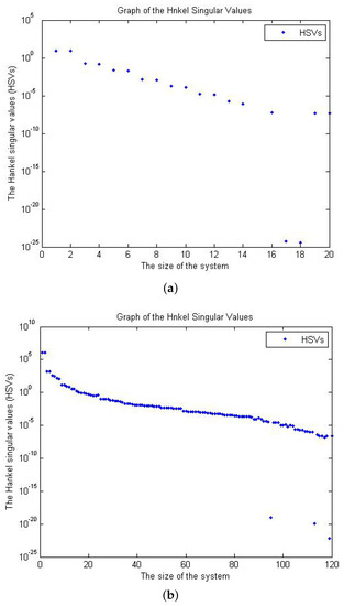
Figure 1. HSVs of the mass–spring damping and CD-player system: (a) HSVs of the mass–spring damping; and (b) HSVs of the CD-player.

For testing purposes, we apply the singular perturbation approximation (SPA) method for the two examples with zero-initial condition and compute the $H^{\infty }$ bound of the approximation error. The size of the mass–spring damping system is taken to be $N_s=10$ and the size of the reduced model is $r_s=2$. Figure 2 shows the maximum singular value decomposition (MSVD) ${\sigma }_{max}$ of $(G-G_r)$, where G is the transfer function of the original system, $G_r$ is the transfer function of the reduced order model, and the error bound is $2{\displaystyle \sum _{i=3}^{10}}{\sigma }_i$.

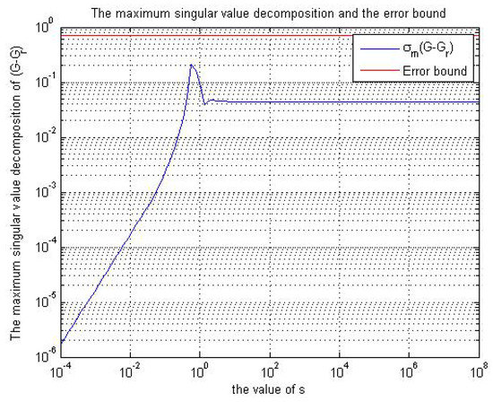
Figure 2. The MSVD and the error bound for the mass–spring damping for the singular perturbation approximation method.

Table 1 contains the values of $\parallel G-G_r{\parallel }_{\infty }$ and $2{\displaystyle \sum _{i=r+1}^{10}}{\sigma }_i$ computed for $N_s=10$ and various values of $r_s$ by applying the balanced truncation and singular perturbation approximation to the mass–spring damping system.

Table 1. The $H^{\infty }$ norm of $(G-G_r)$ and the error bound.

${\mathit{r}}_{\mathit{s}}$	$\parallel \mathit{G}-{\mathit{G}}_{\mathit{r}}{\parallel }_{\mathit{\infty }}$ by SPA	$2{\displaystyle \sum _{\mathit{i}=\mathit{r}+1}^{10}}{\mathit{\sigma }}_{\mathit{i}}$
2	0.2147	0.7025
4	0.0374	0.0873
6	0.0023	0.0061
8	2.6374 $\times {10}^{-4}$	6.7187 $\times {10}^{-4}$
10	2.5247 $\times {10}^{-5}$	6.4759 $\times {10}^{-5}$

To find an error bound for the CD-player, we take the size of the system to be $N_c=120$ and for the reduced model is $r_c=14$. By applying the singular perturbation approximation method, the maximum singular value decomposition of $(G-G_r)$ and the error bound $2{\displaystyle \sum _{i=9}^{120}}{\sigma }_i$ are shown in Figure 3.

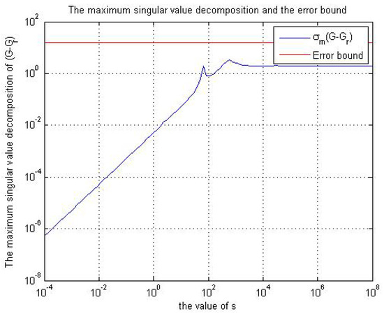
Figure 3. The MSVD and the error bound for the CD-player for the singular perturbation approximation.

Table 2 contains the values of $\parallel G-G_r{\parallel }_{\infty }$ and the error bound $2{\displaystyle \sum _{i=r+1}^{120}}{\sigma }_i$ computed for $N_c=120$ and various $r_c$ by using singular perturbation approximation techniques to the CD-player system.

Table 2. The $H^{\infty }$ norm of $(G-G_r)$ and the error bound.

${\mathit{r}}_{\mathit{c}}$	by SPA	$2{\displaystyle \sum _{\mathit{i}=\mathit{r}+1}^{120}}{\mathit{\sigma }}_{\mathit{i}}$
2	1.1726 $\times {10}^3$	8.8112 $\times {10}^3$
4	564.2177	2.1307 $\times {10}^3$
6	266.4908	658.1466
8	21.9202	117.6033
10	10.9294	63.0871
12	3.3050	30.4559
14	3.3658	15.9412
16	1.7800	10.3588

We see clearly that the singular perturbation approximation produces a reduced order model with an error tends to zero at low frequencies but the error becomes larger at high frequencies.

Next, we want to compute the $L^2$ bound of the approximation error between the output y of the original system and the output $y_r$ of the reduced system with non-zero initial condition. By applying singular perturbation approximation of the reduced order model, we have the formulas for the error bound in Equation (26) denoted by $Erro{r}_{spa}$.

Figure 4 and Figure 5 contain the output y of the original system, the output $y_r$ of the reduced model and the difference $y-y_r$. For the mass spring damping, let $N_s=10$ and $r_s=2$, and for the CD-player $N_c=120$ and $r_c=14$.

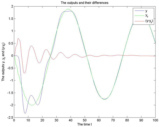
Figure 4. The outputs of the mass–spring damping for SPA.

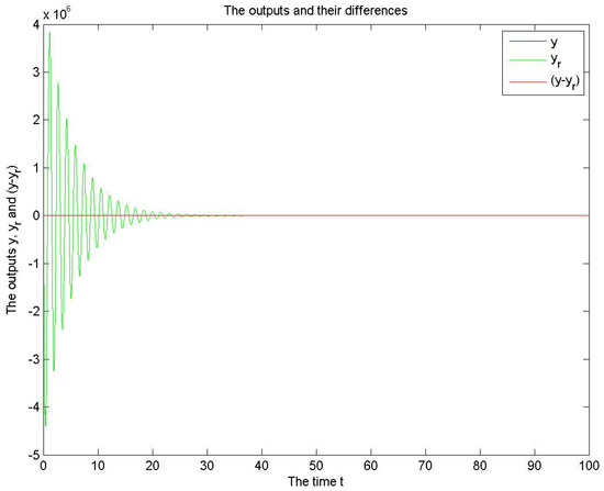
Figure 5. The outputs of the CD-player for SPA.

The $L^2$ norm of $(y-y_r)$ can be computed for different $r_s$. Table 3 and Table 4 contain the values of $\parallel y-y_r{\parallel }_{L_2}$ and the error bounds for the mass–spring damping and the CD-player systems.

Table 3. The $L^2$ norm of $y-y_r$ and the error bounds of the mass–spring damping.

${\mathit{r}}_{\mathit{s}}$	$\parallel \mathit{y}-{\mathit{y}}_{\mathit{r}}{\parallel }_{{\mathit{L}}_2}$ SPA	${\mathit{Error}}_{\mathit{spa}}$
2	1.4448 $\times {10}^{-7}$	0.7845
4	1.3092 $\times {10}^{-10}$	0.0975
6	7.8119 $\times {10}^{-11}$	0.0068
8	2.3580 $\times {10}^{-13}$	7.5161$\times {10}^{-4}$
10	6.2379 $\times {10}^{-15}$	7.3692$\times {10}^{-5}$

Table 4. The $L^2$ norm of $y-y_r$ and the error bounds of the CD-player.

${\mathit{r}}_{\mathit{c}}$	$\parallel \mathit{y}-{\mathit{y}}_{\mathit{r}}{\parallel }_{{\mathit{L}}_2}$ SPA	${\mathit{Error}}_{\mathit{spa}}$
2	530.9562	1.3932$\times {10}^4$
4	13.6649	3.3690$\times {10}^4$
6	13.6595	1.0406$\times {10}^3$
8	1.0136$\times {10}^{-4}$	185.9503
10	2.6581$\times {10}^{-4}$	99.7527
22	1.4723$\times {10}^{-6}$	5.1515
30	4.9888$\times {10}^{-8}$	1.2801

Table 4 contains the $\parallel y-y_r{\parallel }_{L_2}$ norm and the error bounds for the CD-player system.

6. Conclusions

In this thesis, we have studied balanced model reduction techniques for linear control systems, specifically balanced truncation and singular perturbation approximation. These methods have been successfully applied for systems with homogeneous initial conditions but little attention has been paid to systems with inhomogeneous initial conditions or feedback systems.

For open-loop control problems, we have derived an $L^2$ error bound for singular perturbation approximation for system with non-homogeneous initial condition. The theoretical results have been validated numerically.

References

- Alvarez, O.; Bardi, M. Viscosity solutions methods for singular perturbations in deterministic and stochastic control. SIAM J. Control Optim. 2002, 40, 1159–1188. [Google Scholar] [CrossRef]
- Bensoussan, A.; Blankenship, G. Singular perturbations in stochastic control. In Singular Perturbations and Asymptotic Analysis in Control Systems; Springer: Berlin, Germany, 1987; pp. 171–260. [Google Scholar]
- Evans, L.C. The perturbed test function method for viscosity solutions of nonlinear PDE. Proc. R. Soc. Edinb. Sect. A Math. 1989, 111, 359–375. [Google Scholar] [CrossRef]
- Lions, P.L.; Souganidis, P.E. Correctors for the homogenization of Hamilton-Jacobi equations in the stationary ergodic setting. Commun. Pure Appl. Math. 2003, 56, 1501–1524. [Google Scholar] [CrossRef]
- Enns, D.F. Model reduction with balanced realizations: An error bound and a frequency weighted generalization. In Proceedings of the 23rd IEEE Conference on the Decision and Control, Las Vegas, NV, USA, 12–14 December 1984; pp. 127–132. [Google Scholar]
- Skogestad, S.; Postlethwaite, I. Multivariable Feedback Control: Analysis and Design; Wiley: New York, NY, USA, 2007; Volume 2. [Google Scholar]
- Muscato, G.; Nunnari, G.; Fortuna, L. Singular perturbation approximation of bounded real balanced and stochastically balanced transfer matrices. Int. J. Control 1997, 66, 253–270. [Google Scholar] [CrossRef]
- Curtain, R.F.; Glover, K. An Introduction to Infinite-Dimensional Systems; Springer: New York, NY, USA, 1995. [Google Scholar]
- O’Malley, R., Jr. The singularly perturbed linear state regulator problem. SIAM J. Control 1972, 10, 399–413. [Google Scholar] [CrossRef]
- O’Malley, R.E., Jr. On two methods of solution for a singularly perturbed linear state regulator problem. SIAM Rev. 1975, 17, 16–37. [Google Scholar] [CrossRef]
- Daraghmeh, A. Model Order Reduction of Linear Control Systems: Comparison of Balanced Truncation and Singular Perturbation Approximation with Application to Optimal Control. Ph.D. Thesis, Berlin Freie Universität, Berlin, Germany, 2016. [Google Scholar]
- Liu, Y.; Anderson, B.D.O. Singular perturbation approximation of balanced systems. Int. J. Control 1989, 50, 1379–1405. [Google Scholar] [CrossRef]
- Škatarić, D.; Kovačević-Ratković, N. The system order reduction via balancing in view of the method of singular perturbation. FME Trans. 2010, 38, 181–187. [Google Scholar]
- Zhou, K.; Doyle, J.C.; Glover, K. Robust and Optimal Control; Prentice Hall: Upper Saddle River, NJ, USA, 1998. [Google Scholar]
- Antoulas, A.C. Approximation of Large-Scale Dynamical Systems. In Advances in Design and Control; Society for Industrial and Applied Mathematics: Philadelphia, PA, USA, 2005. [Google Scholar]
- Hartmann, C.; Schäfer-Bung, B.; Thöns-Zueva, A. Balanced Averaging of Bilinear Systems with Applications to Stochastic Control. SIAM J. Control Optim. 2013, 51, 2356–2378. [Google Scholar] [CrossRef]
- Saragih, R.; Fatmawati. Singular perturbation approximation of balanced infinite-dimentional system. Int. J. Control Autom. 2013, 6, 409–420. [Google Scholar] [CrossRef]
© 2018 by the authors. Licensee MDPI, Basel, Switzerland. This article is an open access article distributed under the terms and conditions of the Creative Commons Attribution (CC BY) license (http://creativecommons.org/licenses/by/4.0/).