Solution for the System of Lane–Emden Type Equations Using Chebyshev Polynomials

Abstract

In this paper, we use the collocation method together with Chebyshev polynomials to solve system of Lane–Emden type (SLE) equations. We first transform the given SLE equation to a matrix equation by means of a truncated Chebyshev series with unknown coefficients. Then, the numerical method reduces each SLE equation to a nonlinear system of algebraic equations. The solution of this matrix equation yields the unknown coefficients of the solution function. Hence, an approximate solution is obtained by means of a truncated Chebyshev series. Also, to show the applicability, usefulness, and accuracy of the method, some examples are solved numerically and the errors of the solutions are compared with existing solutions.

1. Introduction

In this paper, we consider the system of the Lane–Emden type equation,

$$\begin{array}{l}P(t)\frac{d^2{y}_1}{d{t}^2}+\frac{\alpha }{t}\frac{d{y}_1}{dt}+y_2^p=g_1(t)\\ H(t)\frac{d^2{y}_2}{d{t}^2}+\frac{\beta }{t}\frac{d{y}_2}{dt}+y_1^q=g_2(t)\end{array}$$

(1)

which are subject to the initial conditions,

$$y_1(0)={\lambda }_0, y_1^{\prime }(0)={\lambda }_1 y_2(0)={\gamma }_0, y_2^{\prime }(0)={\gamma }_1$$

(2)

where $p,q$ are positive integers and ${\lambda }_0$, ${\lambda }_1$, ${\gamma }_0$ and ${\gamma }_1$ are real constants. Notice that the Lane–Emden equation is linear for $q=0,1$ and nonlinear otherwise.

There are two basic forms of the the Lane–Emden equation in applied sciences [1,2,3,4,5]. The following equation, which is called the first type Lane–Emden equation, was used to model the problem of stellar structure and the thermal behaviour of a spherical cloud of gas acting under mutual attraction of its molecules [1,2,3,4,5].

$$y^{″}(t)+\frac{2}{t}{y}^{\prime }(t)+g(y)=0,x>0$$

where $g(y)$ is some given function of $y$. Among the most popular form of $g(y)$ is $g(y)=y^m$ with the conditions $y(0)=1$, $y^{\prime }(0)=0$. The exponent $m$ is called polytropic index and positive radially symmetric solutions of the above equation are used to describe the structure of the polytropic stars [1,2,3,4].

The second kind Lane–Emden equation is defined as follows:

$$y^{″}(t)+\frac{2}{t}{y}^{\prime }(t)-e^{-y}=0, y(0)=1,y^{\prime }(0)=0$$

which is used to model the star as a gaseous sphere in thermodynamic and hydrostatic equilibrium with a certain equation of state [2,4].

Several methods for the solution of Lane–Emden equations and the system of Lane–Emden equations have been presented, such as the sinc-collocation method [6], variational iteration method [7], Hermite collocation method [8], modified Homotopy analysis method [9], modified Adomian decomposition method [10], Legendre operational matrix method [11], and Berstein operational matrix method [12], among other methods [13,14,15,16,17].

Recently, the collocation method has been a very useful method to obtain the approximate solutions. Chebyshev collocation method has been used to obtain the numerical solutions to many other equations, such as differential-difference equations, delay-difference equations, pantograph equations, integro-differential-difference equations, and Abel equation, among others [18,19,20,21,22,23,24,25,26,27].

The aim of this study is to get approximate solutions as truncated Chebyshev series defined by

$$y_1^N(t)={\displaystyle \sum _{n=0}^N{}^{\prime }{a}_n{T}_n^{\ast }(t)}, y_2^N(t)={\displaystyle \sum _{n=0}^N{}^{\prime }{b}_n{T}_n^{\ast }(t)}$$

(3)

where $T_n^{\ast }(t)=\cos (n\theta )$, $2t-1=\cos \theta$, $0\le t\le 1$, denotes the shifted Chebyshev polynomials of the first kind; ${\displaystyle \sum {}^{\prime }}$ denotes a sum whose first term is halved; $a_n, b_n (0\le n\le N)$ are unknown Chebyshev coefficients, and $N$ is chosen any positive integer. To obtain a solution of the form Equation (3) of the problem Equation (1) with boundary conditions given by Equation (2), we can use collocation points [28,29].

$$t_{i-1}=\frac{1}{2}\left(1+\cos (\frac{(N-i+3/2)\pi }{N})\right), i=1,2,\dots ,N+1$$

(4)

which is the zeroes of the shifted Chebyshev polynomial $T_{N+1}^{\ast }(t)$. They are called Chebyshev–Gauss points. If we take these points in an interpolation problem, the obtained result is convergence into the given functions [28,29].

2. Fundamental Relations

In this section, we give the matrix form of Equations (1) and (2). Firstly, we convert the solution $y_{1,2}^N(t)$ defined by Equation (3) and its derivative ${\left(y_{1,2}^N(t)\right)}^{(k)}$ to matrix forms

$$y_1^N(t)={\mathbf{T}}^{\ast }(t)\mathbf{A}, y_1^{N(k)}(t)={\mathbf{T}}^{\ast (k)}(t)\mathbf{A}, k=0,1,2$$

(5)

$$y_2^N(t)={\mathbf{T}}^{\ast }(t)\mathbf{B}, y_2^{N(k)}(t)={\mathbf{T}}^{\ast (k)}(t)\mathbf{B}, k=0,1,2$$

(6)

where

$${\mathbf{T}}^{\ast }(t)=[T_0^{\ast }(t) T_1^{\ast }(t) \dots T_N^{\ast }(t)],$$

$${\mathbf{T}}^{\ast (k)}(t)=[T_0^{\ast (k)}(t) T_1^{\ast (k)}(t) \dots T_N^{\ast (k)}(t)],$$

$$\mathbf{A}=[\frac{1}{2}{a}_0 a_1\dots a_N{]}^T,$$

$$\mathbf{B}=[\frac{1}{2}{b}_0 b_1\dots b_N{]}^T.$$

On the other hand, it has been known that the relation between the powers tⁿ and the shifted Chebyshev polynomials $T_n^{\ast }\left(t\right)$ is [24,25].

$$t^n=2^{-2n+1}{\displaystyle \sum _{k=0}^n{}^{\prime }}\left(\begin{array}{l}2n\\ k\end{array}\right)T_{n-k}^{\ast }(t), 0\le t\le 1$$

(7)

Using the expression (7) and taking n = 0, 1, …, N, we find the corresponding matrix relation as follows:

$${(\mathbf{X}(t))}^T=\mathbf{D}{({\mathbf{T}}^{\ast }(t))}^T\hspace{1em}implying\hspace{1em}that\hspace{1em}\mathbf{X}(t)={\mathbf{T}}^{\ast }(t){\mathbf{D}}^T$$

(8)

where

$$\mathbf{X}(t)=[1 t \dots t^N]$$

which is a lower triangular matrix. As all the main diagonals of $\mathbf{D}$ are not zero, $\mathbf{D}$ is invertible matrix. Then, taking into account Equation (8), we obtain

$${\mathbf{T}}^{\ast }(t)=\mathbf{X}(t){({\mathbf{D}}^{-1})}^T$$

(9)

and

$${({\mathbf{T}}^{\ast }(t))}^{(k)}={\mathbf{X}}^{(k)}(t){({\mathbf{D}}^{-1})}^T, k=0,1,2$$

We use the following relation to obtain the matrix ${\mathbf{X}}^{(k)}(t)$ in terms of the matrix $\mathbf{X}(t),$

$${\mathbf{X}}^{(1)}(t)=\mathbf{X}(t){\mathbf{C}}^T,$$

$${\mathbf{X}}^{(2)}(t)={\mathbf{X}}^{(1)}(t){\mathbf{C}}^T=\mathbf{X}(t){({\mathbf{C}}^T)}^2$$

(10)

where

$$\mathbf{C}=\left[\begin{array}{ccccc}0& 0& 0& \dots & 0\\ 1& 0& 0& \dots & 0\\ 0& 2& 0& \dots & 0\\ \dots & \dots & \dots & \dots & \dots \\ 0& 0& 0& N& 0\end{array}\right].$$

Consequently, by substituting the matrix forms Equations (9) and (10) into Equations (5) and (6), we have the matrix relation

$$y_1^{N(k)}(t)=\mathbf{X}(t){\mathbf{C}}^k{({\mathbf{D}}^T)}^{-1}\mathbf{A}, k=0,1,2$$

(11)

$$y_2^{N(k)}(t)=\mathbf{X}(t){\mathbf{C}}^k{({\mathbf{D}}^T)}^{-1}\mathbf{B}, k=0,1,2$$

(12)

Now, we construct the matrix form of the nonlinear term ${\left(y_1^N(t)\right)}^q$ and ${\left(y_2^N(t)\right)}^p$, substituting the collocation points into ${\left(y_1^N(t)\right)}^q$, we obtain the following matrix representation

$$\left[\begin{array}{c}{\left(y_1^N(t_0)\right)}^q\\ {\left(y_1^N(t_1)\right)}^q\\ ⋮\\ {\left(y_1^N(t_N)\right)}^q\end{array}\right]={\left[\begin{array}{cccc}{y}_1^N(t_0)& 0& 0& 0\\ 0& y_1^N(t_1)& 0& 0\\ ⋮& ⋮& \ddots & ⋮\\ 0& 0& 0& y_1^N(t_N)\end{array}\right]}^{q-1}\left[\begin{array}{c}{y}_1^N(t_0)\\ y_1^N(t_1)\\ ⋮\\ y_1^N(t_N)\end{array}\right]={\left(\overline{{\mathbf{Y}}_1}\right)}^{\mathbf{q}-\mathbf{1}}{\mathbf{Y}}_{\mathbf{1}}$$

(13)

and

$$\overline{{\mathbf{Y}}_1}=\overline{\mathbf{T}}\overline{\mathbf{A}}$$

(14)

where

$$\overline{\mathbf{T}}=\left[\begin{array}{cccc}\mathbf{T}(t_0)& 0& \cdots & 0\\ 0& \mathbf{T}(t_1)& \cdots & 0\\ ⋮& ⋮& \ddots & ⋮\\ 0& 0& \cdots & \mathbf{T}(t_N)\end{array}\right], \overline{\mathbf{A}}=\left[\begin{array}{cccc}\mathbf{A}& 0& \cdots & 0\\ 0& \mathbf{A}& \cdots & 0\\ ⋮& ⋮& \ddots & ⋮\\ 0& 0& \cdots & \mathbf{A}\end{array}\right]$$

Then, we construct the following matrix relation

$${\left(y_1^N(t)\right)}^q={\left(y_1^N(t)\right)}^{q-1}\left(y_1^N(t)\right)1={(\overline{\mathbf{T}}\overline{\mathbf{A}})}^{q-1}\mathbf{X}(t){{(\mathbf{D}}^{\mathbf{T}})}^{-1}\mathbf{A}$$

(15)

Similarly, ${\left(y_2^N(t)\right)}^p$ can be written as

$${\left(y_2^N(t)\right)}^p={\left(y_2^N(t)\right)}^{p-1}\left(y_2^N(t)\right)={(\overline{\mathbf{T}}\overline{\mathbf{B}})}^{p-1}\mathbf{X}(t){{(\mathbf{D}}^{\mathbf{T}})}^{-1}\mathbf{B}$$

(16)

where

$$\overline{\mathbf{B}}=\left[\begin{array}{cccc}\mathbf{B}& 0& \cdots & 0\\ 0& \mathbf{B}& \cdots & 0\\ ⋮& ⋮& \ddots & ⋮\\ 0& 0& \cdots & \mathbf{B}\end{array}\right]$$

3. Method of Solution

In this section, the fundamental matrix equation corresponding to Equation (1) with conditions Equation (2) is constructed, and the solution method is presented. For this purpose, we substitute the matrix relations Equations (11),(12) and Equations (15),(16) into Equation (1) and obtain the following matrix relation:

$$\begin{array}{l}{P}_1(t)\mathbf{X}(t){\mathbf{C}}^2{({\mathbf{D}}^T)}^{-1}\mathbf{A}+\frac{\alpha }{t}\mathbf{X}(t)\mathbf{C}{({\mathbf{D}}^T)}^{-1}\mathbf{A}+{(\overline{\mathbf{T}}\overline{\mathbf{B}})}^{p-1}\mathbf{X}(t){\left({\mathbf{D}}^{\mathbf{T}}\right)}^{-1}\mathbf{B}=g_1(t)\\ P_2(t)\mathbf{X}(t){\mathbf{C}}^2{({\mathbf{D}}^T)}^{-1}\mathbf{B}+\frac{\beta }{t}\mathbf{X}(t)\mathbf{C}{({\mathbf{D}}^T)}^{-1}\mathbf{B}+{(\overline{\mathbf{T}}\overline{\mathbf{A}})}^{q-1}\mathbf{X}(t){\left({\mathbf{D}}^{\mathbf{T}}\right)}^{-1}\mathbf{A}=g_2(t)\end{array},$$

(17)

We can rewrite the Equation (17) as follows:

$$\mathbf{P}(t)\overline{\mathbf{X}}(t)\overline{\overline{\mathbf{C}}}\overline{\mathbf{D}}\mathbf{Y}+\mathbf{H}(t)\overline{\mathbf{X}}(t)\overline{\mathbf{C}}\overline{\mathbf{D}}\mathbf{Y}+\overline{\mathbf{T}}(t)\overline{\overline{\mathbf{X}(t)}}\overline{\overline{\mathbf{D}}}\mathbf{Y}=\mathbf{G}(t)$$

(18)

where

$$\mathbf{P}(t)=\left[\begin{array}{cc}{P}_1(t)& 0\\ 0& P_2(t)\end{array}\right], \overline{\mathbf{X}}(t)=\left[\begin{array}{cc}\mathbf{X}(t)& 0\\ 0& \mathbf{X}(t)\end{array}\right], \overline{\overline{\mathbf{C}}}=\left[\begin{array}{cc}{\mathbf{C}}^2& 0\\ 0& {\mathbf{C}}^2\end{array}\right]$$

$$\overline{\mathbf{D}}=\left[\begin{array}{cc}{({\mathbf{D}}^T)}^{-1}& 0\\ 0& {({\mathbf{D}}^T)}^{-1}\end{array}\right], \mathbf{H}(t)=\left[\begin{array}{cc}\alpha /t& 0\\ 0& \beta /t\end{array}\right], \overline{\mathbf{C}}=\left[\begin{array}{cc}\mathbf{C}& 0\\ 0& \mathbf{C}\end{array}\right]$$

$$\overline{\mathbf{T}}(t)=\left[\begin{array}{cc}0& {(\mathbf{T}(t)\mathbf{B})}^{p-1}\\ {(\mathbf{T}(t)\mathbf{A})}^{q-1}& 0\end{array}\right]$$

$$\overline{\overline{\mathbf{X}}}(t)=\left[\begin{array}{cc}0& \mathbf{X}(t)\\ \mathbf{X}(t)& 0\end{array}\right], \overline{\overline{\mathbf{D}}}(t)=\left[\begin{array}{cc}0& {({\mathbf{D}}^T)}^{-1}\\ {({\mathbf{D}}^T)}^{-1}& 0\end{array}\right], \mathbf{Y}=\left[\begin{array}{c}\mathbf{A}\\ \mathbf{B}\end{array}\right], \mathbf{G}(t)=\left[\begin{array}{c}{g}_1(t)\\ g_2(t)\end{array}\right].$$

Using collocation points, we get the matrix equations

$$\left(\mathbf{P}\overline{\mathbf{X}}\overline{\overline{\mathbf{C}}}\overline{\mathbf{D}}+\mathbf{H}\overline{\mathbf{X}}\overline{\mathbf{C}}\overline{\mathbf{D}}+\overline{\mathbf{T}}\overline{\overline{\mathbf{X}}}\overline{\overline{\mathbf{D}}}\right)\mathbf{Y}=\mathbf{G}$$

(19)

where

$$\mathbf{P}=\left[\begin{array}{ccccc}\mathbf{P}(t_0)& 0& 0& \cdots & 0\\ 0& \mathbf{P}(t_1)& 0& \cdots & 0\\ 0& 0& \mathbf{P}(t_2)& \cdots & 0\\ ⋮& ⋮& ⋮& \ddots & ⋮\\ 0& 0& 0& \cdots & \mathbf{P}(t_N)\end{array}\right], \mathbf{H}=\left[\begin{array}{ccccc}\mathbf{H}(t_0)& 0& 0& \cdots & 0\\ 0& \mathbf{H}(t_1)& 0& \cdots & 0\\ 0& 0& \mathbf{H}(t_2)& \cdots & 0\\ ⋮& ⋮& ⋮& \ddots & ⋮\\ 0& 0& 0& \cdots & \mathbf{H}(t_N)\end{array}\right], \mathbf{C}=\left[\begin{array}{ccccc}0& 0& 0& \dots & 0\\ 1& 0& 0& \dots & 0\\ 0& 2& 0& \dots & 0\\ \dots & \dots & \dots & \dots & \dots \\ 0& 0& 0& N& 0\end{array}\right]$$

$$\overline{\mathbf{D}}=\left[\begin{array}{cc}{({\mathbf{D}}^T)}^{-1}& 0\\ 0& {({\mathbf{D}}^T)}^{-1}\end{array}\right], \mathbf{Y}=\left[\begin{array}{c}\mathbf{A}\\ \mathbf{B}\end{array}\right], \overline{\overline{\mathbf{D}}}=\left[\begin{array}{cc}\overline{\mathbf{D}}& 0\\ 0& \overline{\mathbf{D}}\end{array}\right]$$

$$\overline{\mathbf{X}}=\left[\begin{array}{ccccc}\overline{\mathbf{X}}(t_0)& 0& 0& \cdots & 0\\ 0& \overline{\mathbf{X}}(t_1)& 0& \cdots & 0\\ 0& 0& \overline{\mathbf{X}}(t_2)& \cdots & 0\\ ⋮& ⋮& ⋮& \ddots & ⋮\\ 0& 0& 0& \cdots & \overline{\mathbf{X}}(t_N)\end{array}\right], \overline{\mathbf{T}}=\left[\begin{array}{ccccc}\overline{\mathbf{T}}(t_0)& 0& 0& \cdots & 0\\ 0& \overline{\mathbf{T}}(t_1)& 0& \cdots & 0\\ 0& 0& \overline{\mathbf{T}}(t_2)& \cdots & 0\\ ⋮& ⋮& ⋮& \ddots & ⋮\\ 0& 0& 0& \cdots & \overline{\mathbf{T}}(t_N)\end{array}\right]$$

$$\overline{\overline{\mathbf{X}}}=\left[\begin{array}{ccccc}\overline{\overline{X}}(t_0)& 0& 0& \cdots & 0\\ 0& \overline{\overline{X}}(t_1)& 0& \cdots & 0\\ 0& 0& \overline{\overline{X}}(t_2)& \cdots & 0\\ ⋮& ⋮& ⋮& \ddots & ⋮\\ 0& 0& 0& \cdots & \overline{\overline{X}}(t_N)\end{array}\right], \mathbf{G}=\left[\begin{array}{c}G(t_0)\\ G(t_1)\\ G(t_2)\\ ⋮\\ G(t_N)\end{array}\right]$$

and where

$$\overline{\mathbf{X}}(t_i)=\left[\begin{array}{cc}\mathbf{X}(t_i)& 0\\ 0& \mathbf{X}(t_i)\end{array}\right], \mathbf{P}(t_i)=\left[\begin{array}{cc}{P}_1(t_i)& 0\\ 0& P_2(t_i)\end{array}\right], \mathbf{H}(t_i)=\left[\begin{array}{cc}\alpha /t_i& 0\\ 0& \beta /t_i\end{array}\right]$$

$$\overline{\mathbf{T}}(t_i)=\left[\begin{array}{cc}0& {(\mathbf{T}(t_i)\mathbf{B})}^{p-1}\\ {(\mathbf{T}(t_i)\mathbf{A})}^{q-1}& 0\end{array}\right], \overline{\overline{\mathbf{X}}}(t_i)=\left[\begin{array}{cc}0& \mathbf{X}(t_i)\\ \mathbf{X}(t_i)& 0\end{array}\right], \mathbf{G}(t_i)=\left[\begin{array}{c}{g}_1(t_i)\\ g_2(t_i)\end{array}\right].$$

where the dimension of matrices $\overline{\mathbf{X}}$, $\overline{\overline{\mathbf{X}}}$, $\overline{\overline{\mathbf{C}}}$, $\overline{\mathbf{C}}$, $\overline{\overline{\mathbf{D}}}$, $\overline{\mathbf{D}}$, $\overline{\mathbf{T}}$ are diagonal matrices and the dimension of these matrices are $2(N+1)\times 2(N+1)$ and $\mathbf{G}$ is $2(N+1)\times 1$.

Hence, the matrix Equation (19) corresponding to Equation (1) can be written in the form

$$\mathbf{WY}=\mathbf{G},$$

(20)

where

$$\mathbf{W}=\mathbf{P}\overline{\mathbf{X}}\overline{\overline{\mathbf{C}}}\overline{\mathbf{D}}+\mathbf{H}\overline{\mathbf{X}}\overline{\mathbf{C}}\overline{\mathbf{D}}+\overline{\mathbf{T}}\overline{\overline{\mathbf{X}}}\overline{\overline{\mathbf{D}}}$$

Moreover, the matrix form for conditions can be written as

$${\mathbf{U}}_0=\mathbf{X}(0){({\mathbf{D}}^T)}^{-1}\mathbf{A}=\left[{\lambda }_0\right],$$

$${\mathbf{U}}_1=\mathbf{X}(0)\mathbf{C}{({\mathbf{D}}^T)}^{-1}\mathbf{A}=\left[{\lambda }_1\right],$$

$${\mathbf{U}}_2=\mathbf{X}(0){({\mathbf{D}}^T)}^{-1}\mathbf{B}=\left[{\alpha }_0\right],$$

$${\mathbf{U}}_3=\mathbf{X}(0)\mathbf{C}{({\mathbf{D}}^T)}^{-1}\mathbf{B}=\left[{\alpha }_1\right],$$

where

$$\mathbf{X}\left(0\right)=[1\hspace{1em}0\hspace{1em}0\hspace{1em}0\hspace{1em}0\hspace{1em}0]$$

Then, we can write the conditions as the following matrix form:

$$\mathbf{UY}=\mathbf{F},$$

(21)

where

$$\mathbf{U}=[u_{kl}]=\left[\begin{array}{cc}{\mathbf{U}}_0& 0\\ {\mathbf{U}}_1& 0\\ 0& {\mathbf{U}}_2\\ 0& {\mathbf{U}}_3\end{array}\right], \mathbf{F}=\left[\begin{array}{c}{\lambda }_0\\ {\lambda }_1\\ {\alpha }_0\\ {\alpha }_1\end{array}\right]$$

By replacing the conditions matrices (20) by the last four rows of the matrix (21), we obtain to a system of $2(N+1)\times 2(N+1)$ linear or nonlinear algebraic equations with $2(N+1)$ unknown Chebyshev coefficients. Thereby, the unknown coefficients matrix $\mathbf{A}$ and $\mathbf{B}$ are obtained by solving the system by aid of Maple 13. Consequently, by replacing the obtained coefficients $a_n, b_n$ into Equation (3), we have the wanted approximate solution of Equation (1).

4. Algorithm

In this section, we give the algorithm of the proposed method (see also [26]).

Step 1. Our input data: $P(t),H(t)$, $g_1(t),g_2(t)$ and conditions.

Step 2. Select $N$.

Step 3. Construct the matrices ${\mathbf{T}}^{\ast }(t)$,$\mathbf{X}(t), {({\mathbf{D}}^{-1})}^T$, $\mathbf{C}$, $\mathbf{A}$, $\mathbf{B}$, $\mathbf{P},\overline{\mathbf{X}},\overline{\overline{\mathbf{C}}},\overline{\mathbf{D}},\mathbf{H},\overline{\mathbf{X}},\overline{\mathbf{C}},$ $\overline{\mathbf{D}},\overline{\mathbf{T}},\overline{\overline{\mathbf{X}}},\overline{\overline{\mathbf{D}}}$.

Step 4. Determine the collocation points: $t_{i-1}=\frac{1}{2}\left(1+\cos (\frac{(N-i+3/2)\pi }{N})\right)$.

Step 5. Compute $\mathbf{U}$, $\mathbf{F}$.

Step 6. Construct the system.

Step 7. On the proposed of finding $\mathbf{A},\mathbf{B}$, solve the obtained system by aid of Maple 13.

Step 8. Put the coefficients of truncated Chebyshev series in the truncated Chebyshev series.

Step 9. Out put data: the approximate solutions $y_1(t)$, $y_2(t)$.

5. Examples

In this section, several numerical examples are given to illustrate the accuracy and effectiveness properties of the method and all of them were performed on the computer using a program written in Maple 13. To study the behavior of the present method, we applied the following laws:

(1) Absolute error ($N_e$) is defined by the following:

$$N_e(t_i)=\left|y_j(t_i)-y_j^N(t_i)\right|, t_i\in [0,1], j=1,2$$

(22)

where $y_j(x)$ are the exact solutions and $y_j^N(x)$ denote the approximate solution obtained by the present method.

(2) Relative error, which is defined by the following:

$$relN=\frac{\left|y_j(t_i)-y_j^N(t_i)\right|}{\left|y_j(t_i)\right|}, t_i\in [0,1], j=1,2$$

(3)

$$E_N^L={\left({\displaystyle \underset{0}{\overset{1}{\int }}{\left(y_j(t)-y_j^N(t)\right)}^{2}dt}\right)}^{1/2}, j=1,2$$

where $y_j(x)$ are the exact solutions and denote the approximate solution obtained by the present method.

Example 1.

Let us consider the following linear systems of Lane–Emden equations

$$\begin{array}{l}{y}_1^{″}+\frac{3}{t}{y}_1^{\prime }-4(y_1+y_2)=0\\ y_2^{″}+\frac{2}{t}{y}_2^{\prime }+3(y_1+y_2)=0\end{array}$$

(23)

subject to initial conditions

$$y_1(0)=1, y_2(0)=1, y_1^{\prime }(0)=0, y_2^{\prime }(0)=0$$

which approximates a fully convective star, that is, a very cool late-type star.

Then,

$$\mathbf{P}(t)=\left[\begin{array}{cc}1& 0\\ 0& 1\end{array}\right], \mathbf{H}(t)=\left[\begin{array}{cc}3/t& 0\\ 0& 2/t\end{array}\right], \mathbf{R}(t)=\left[\begin{array}{cc}-4& -4\\ 3& 3\end{array}\right], \mathbf{G}(t)=\left[\begin{array}{c}0\\ 0\end{array}\right]$$

Now, we can apply our technique described in Section 3 for $N=5$; that is, we seek the approximate solution of Equation (23) for $N=5$ by the terms of truncated Chebyshev polynomial series as

$$y_1^5(t)={\displaystyle \sum _{n=0}^5{}^{\prime }{a}_n{T}_n^{\ast }(t)}{y}_2^5(t)={\displaystyle \sum _{n=0}^5{}^{\prime }{b}_n{T}_n^{\ast }(t)}$$

For $N=5$, the Chebyshev–Gaus grid points are

$$t_0=\frac{1}{2}-\frac{1}{2}\cos (\frac{\pi }{12}), t_1=\frac{1}{2}-\frac{\sqrt{2}}{4}, t_2=\frac{1}{2}-\frac{1}{2}\cos (\frac{5\pi }{12}), t_3=\frac{1}{2}+\frac{1}{2}\cos (\frac{\pi }{12})$$

$$t_4=\frac{1}{2}+\frac{\sqrt{2}}{4}, t_5=\frac{1}{2}+\frac{1}{2}\cos (\frac{\pi }{12})$$

Then, the matrix form of the problem

$$\left(\mathbf{P}\overline{\mathbf{X}}\overline{\overline{\mathbf{C}}}\overline{\mathbf{D}}+\mathbf{H}\overline{\mathbf{X}}\overline{\mathbf{C}}\overline{\mathbf{D}}+\mathbf{R}\overline{\mathbf{X}}\overline{\mathbf{D}}\right)\mathbf{Y}=\mathbf{G}$$

(24)

where

$$\overline{\mathbf{P}}=\left[\begin{array}{cccccc}{\mathbf{P}}_0& 0& 0& 0& 0& 0\\ 0& {\mathbf{P}}_1& 0& 0& 0& 0\\ 0& 0& {\mathbf{P}}_2& 0& 0& 0\\ 0& 0& 0& {\mathbf{P}}_3& 0& 0\\ 0& 0& 0& 0& {\mathbf{P}}_4& 0\\ 0& 0& 0& 0& 0& {\mathbf{P}}_5\end{array}\right], \mathbf{H}=\left[\begin{array}{cccccc}{\mathbf{H}}_0& 0& 0& 0& 0& 0\\ 0& {\mathbf{H}}_1& 0& 0& 0& 0\\ 0& 0& {\mathbf{H}}_2& 0& 0& 0\\ 0& 0& 0& {\mathbf{H}}_3& 0& 0\\ 0& 0& 0& 0& {\mathbf{H}}_4& 0\\ 0& 0& 0& 0& 0& {\mathbf{H}}_5\end{array}\right], \overline{\mathbf{F}}=\left[\begin{array}{c}{\mathbf{G}}_0\\ {\mathbf{G}}_1\\ {\mathbf{G}}_2\\ {\mathbf{G}}_3\\ {\mathbf{G}}_4\\ {\mathbf{G}}_5\end{array}\right]$$

and where

$${\mathbf{P}}_i=\left[\begin{array}{cc}1& 0\\ 0& 1\end{array}\right], {\mathbf{H}}_i=\left[\begin{array}{cc}3/t_i& 0\\ 0& 2/t_i\end{array}\right], {\mathbf{R}}_i=\left[\begin{array}{cc}-4& -4\\ 3& 3\end{array}\right], {\mathbf{G}}_i=\left[\begin{array}{c}0\\ 0\end{array}\right]$$

$${({\mathbf{D}}^T)}^{-1}=\left[\begin{array}{cccccc}1& -1& 1& -1& 1& -1\\ 0& 2& -8& 18& -32& 50\\ 0& 0& 8& -48& 160& -400\\ 0& 0& 0& 32& -256& 1120\\ 0& 0& 0& 0& 128& -1280\\ 0& 0& 0& 0& 0& 512\end{array}\right], \mathbf{C}=\left[\begin{array}{cccccc}0& 1& 0& 0& 0& 0\\ 0& 0& 2& 0& 0& 0\\ 0& 0& 0& 3& 0& 0\\ 0& 0& 0& 0& 4& 0\\ 0& 0& 0& 0& 0& 5\\ 0& 0& 0& 0& 0& 0\end{array}\right]$$

Moreover, the matrix form for conditions can be written as follows:

$$\left[\begin{array}{c}{y}_1(0)\\ y_2(0)\end{array}\right]\equiv \left[\begin{array}{cc}{\mathbf{U}}_0& \mathbf{0}\\ \mathbf{0}& {\mathbf{U}}_1\end{array}\right]\left[\begin{array}{c}\mathbf{A}\\ \mathbf{B}\end{array}\right]=\left[\begin{array}{c}1\\ 1\end{array}\right]$$

$$\left[\begin{array}{c}{y}_1^{\prime }(0)\\ y_1^{\prime }(0)\end{array}\right]\equiv \left[\begin{array}{cc}{\mathbf{U}}_2& \mathbf{0}\\ \mathbf{0}& {\mathbf{U}}_3\end{array}\right]\left[\begin{array}{c}\mathbf{A}\\ \mathbf{B}\end{array}\right]=\left[\begin{array}{c}0\\ 0\end{array}\right]$$

0_6×1 is zero matrix.

where

$${\mathbf{U}}_0={\mathbf{U}}_1=\mathbf{X}(0){({\mathbf{D}}^T)}^{-1}=\left[\begin{array}{cccccc}1& -1& 1& -1& 1& -1\end{array}\right]$$

$${\mathbf{U}}_2={\mathbf{U}}_3=\mathbf{X}(0){({\mathbf{D}}^T)}^{-1}=\left[\begin{array}{cccccc}0& 2& -8& 18& -32& 50\end{array}\right]$$

Solving the augmented matrix based on conditions, Chebyshev coefficients matrix is obtained as follows:

$$\mathbf{A}=\left[\begin{array}{c}11/8\\ 1/2\\ 1/8\\ 0\\ 0\\ 0\end{array}\right], \mathbf{B}=\left[\begin{array}{c}5/8\\ -1/2\\ -1/8\\ 0\\ 0\\ 0\end{array}\right]$$

Thereby, the solutions of the problem for $N=5$ become

$$y_1^5(t)=1+t^2 \mathrm{and} y_2^5(t)=1-t^2$$

which are the exact solution for Equation (23).

Example 2.

Let us consider the linear, non-homogeneous systems of Lane–Emden equations, which describes polytropes in hydrostatic equilibrium as simple models of a star.

$$\begin{array}{l}{y}_1^{″}(t)+\frac{2}{t}{y}_1^{\prime }(t)-(4t^2+6)y_1(t)+y_2(t)=t^4-t^3\\ y_2^{″}(t)+\frac{8}{t}{y}_2^{\prime }(t)+t{y}_2(t)+y_1(t)=e^{t^2}+t^5-t^4+44t^2-30t\end{array}$$

subject to conditions,

$$y_1(0)=1, y_1^{\prime }(0)=0, y_2(0)=0, y_2^{\prime }(0)=0$$

The exact solutions of above equation are $y_1(t)=t^4-t^3$ and $y_2(t)=e^{t^2}$. The absolute errors which are defined by $\left|y_i(x)-y_i^N(x)\right|,i=1,2$ are shown in Table 1 and Table 2. In Table 3, the computational results of the $L^2$-norm error and truncated errors are summarized. The error in truncating a Chebyshev series by neglecting all terms of degree $N+1$ and higher is bounded by sum of the absolute values of neglected terms [28,29].

$${\max }_{t\in [0,1]}\left|y_j(t)-y_j^N(t)\right|\le {\displaystyle \sum _{n=N+1}^{\infty }\left|a_n\right|=}{E}_N^T (\mathrm{or} b_n)$$

Table 1. Numerical result for approximate solution of $y_1(t)$ in Example 2.

t	Exact Solution	N = 5	Ne = 5	N = 6	Ne = 6	N = 8	Ne = 8
0.0	1.000000	0.999999	0.800 × 10−8	0.999999	0.500 × 10−9	1	0
0.2	1.040810	1.040834	0.238 × 10−4	1.040810	0.135 × 10−6	1.040810	0.102 × 10−6
0.4	1.173510	1.173384	0.126 × 10−3	1.173517	0.690 × 10−5	1.173510	0.261 × 10−6
0.6	1.433329	1.433539	0.209 × 10−3	1.433298	0.305 × 10−4	1.433329	0.471 × 10-6
0.8	1.896480	1.895792	0.688 × 10−2	1.896583	0.102 × 10−3	1.896481	0.909 × 10−6
1.0	2.718281	2.686791	0.314 × 10−1	2.712165	0.611 × 10−3	2.718083	0.197 × 10−3

Table 2. Numerical result for approximate solution of $y_2(t)$ in Example 2.

t	Exact Solution	N = 5	Ne = 5	N = 6	Ne = 6	N = 8	Ne = 8
0	0	0	0	0	0	0	0
0.2	−0.0064	−0.006400	0.436 × 10−7	−0.006400	0.189 × 10−9	−0.00640	0.122 × 10−9
0.4	−0.0384	−0.038399	0.343 × 10−6	−0.038400	0.358 × 10−7	−0.03840	0.399 × 10−9
0.6	−0.0864	−0.086399	0.770 × 10−5	−0.086399	0.102 × 10−6	−0.08640	0.138 × 10−8
0.8	−0.1024	−0.102400	0.620 × 10−5	−0.102400	0.259 × 10−6	−0.10240	0.455 × 10−8
1.0	0.0000	−0.419×10−4	0.419 × 10−4	−0.722×10−5	0.722 × 10−5	0.168 × 10−6	0.168 × 10−6

Table 3. Numerical result for Example 2.

Present Method	${\mathit{E}}_{\mathit{N}}^{\mathit{L}}$		${\mathit{E}}_{\mathit{N}}^{\mathit{T}}$
-	$y_1(t)$	$y_2(t)$	$y_1(t)$	$y_2(t)$
N = 5	0.615773 × 10−2	101474 × 10−4	10−2	10−6
N = 6	0.103500 × 10−2	0.148370 × 10−5	10−3	10−8
N = 8	0.263404 × 10−4	0.256832 × 10−7	10−5	10−10

In Figure 1 and Figure 2, we plot the obtained absolute errors. Figure 3 and Figure 4 give us a comparison of the relative errors. All numerical results and figures are show us the presented method is very successful to obtain approximate solutions with small $N$ values. Note that $E-n={10}^{-n}$.

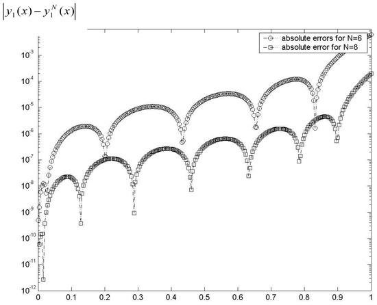
Figure 1. Comparison of absolute errors function for y₁(t).

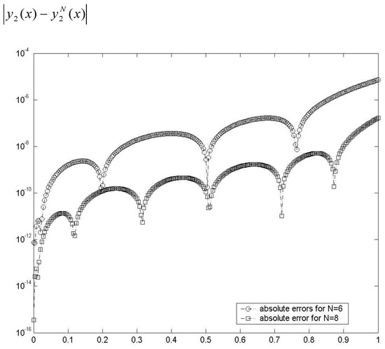
Figure 2. Comparison of absolute errors function for y₂(t).

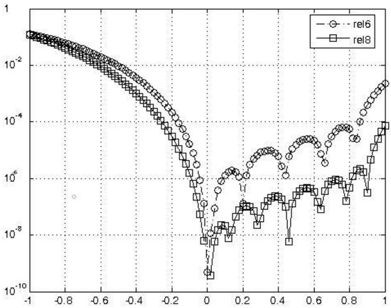
Figure 3. Relative errors of y₁(t).

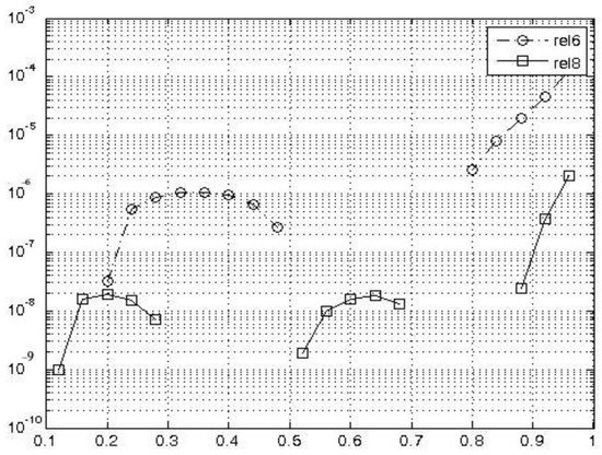
Figure 4. Relative errors of y₂(t).

Example 3.

Lastly, consider the following nonlinear problem [26]:

$$\begin{array}{l}{y}_1^{″}(t)+\frac{1}{t}{y}_1^{\prime }(t)-y_2^3(t)(y_1^2(t)+1)=0\\ y_2^{″}(t)+\frac{3}{t}{y}_2^{\prime }(t)+y_2^5(t)(y_1^2(t)+3)=0\end{array}$$

subject to conditions

$$y_1(0)=1, y_1^{\prime }(0)=1, y_2(0)=0, y_2^{\prime }(0)=0$$

with exact solutions

$$y_1=\sqrt{1+t^2}, y_2=\frac{1}{\sqrt{1+t^2}}$$

Wazwaz et al. [26] has introduced the systematic Adomian decomposition method, which has yielded the exact solution of this problem. Applying our method for $N=4,5,6$, the obtained numerical results are displayed in Table 4 and Table 5. The tables and the figures show that the proposed method is in good agreement with the analytical solution.

Table 4. Numerical result for approximate solution of y₁(t) in Example 3.

t	Exact Solution	N = 4	Ne = 4	N = 5	Ne = 5	N = 6	Ne = 6
0.0	1.00000	1.000000	0	1.00000	0	1.00000	0
0.2	1.019803	1.020423	0.509 × 10−3	1.019815	0.565 × 10−4	1.019803	0.756 × 10−5
0.4	1.077032	1.077135	0.628 × 10−3	1.077064	0.216 × 10−4	1.077032	0.865 × 10−5
0.6	1.166190	1.166724	0.277 × 10−3	1.166185	0.557 × 10−5	1.166190	0.456 × 10−5
0.8	1.280624	1.280663	0.272 × 10−3	1.280699	0.738 × 10−4	1.280624	0.771 × 10−5
1.0	1.414213	1.414742	0.644 × 10−3	1.414217	0.746 × 10−4	1.414213	0.656 × 10−5

Table 5. Numerical result for approximate solution of y₂(t) in Example 3.

t	Exact Solution	N = 4	Ne = 4	N = 5	Ne = 5	N = 6	Ne = 6
0.0	1.000000	1.000000	0	1.000000	0	1.000000	0
0.2	0.980580	0.980103	0.103 × 10−3	0.980570	0.165 × 10−4	0.980580	0.659 × 10−5
0.4	0.928476	0.928687	0.227 × 10−3	0.928466	0.151 × 10−4	0.928476	0.765 × 10−5
0.6	0.857492	0.858961	0.100 × 10−3	0.857482	0.166 × 10−4	0.857492	0.963 × 10−5
0.8	0.780868	0.781652	0.692 × 10−3	0.780898	0.167 × 10−4	0.780868	0.865 × 10−5
1.0	0.707106	0.706123	0.262 × 10−3	0.707146	0.608 × 10−4	0.707106	0.653 × 10−6

6. Conclusions

As the system of the Lane–Emden type equations, which are nonlinear equations and singular, solutions of these types of equation are hardly obtained with the known classical methods. Herein, useful and effective approximate methods are needed. In this article, we deal with obtaining numerical solutions. The numerical method reduces the problem into the system of nonlinear algebraic equations with unknown coefficients. The effectiveness of the method is examined by comparing the obtained results with the exact solutions.

References

- Fowler, R.H. Further studies of Emden’s and similar differential equations. Q. J. Math. 1931, 2, 259–288. [Google Scholar] [CrossRef]
- Meerson, E.; Megged, E.; Tajima, T. On the quasi-hydrostatic flows of radiatively cooling self-gravitating gas clouds. Astrophys. J. 1996, 457, 321. [Google Scholar] [CrossRef]
- Chandrasekhar, S. Introduction to Study of Stellar Structure. Available online: https://www.amazon.com/Introduction-Study-Stellar-Structure-Astronomy/dp/0486604136 (accessed on 22 August 2018).
- Davis, H.T. Introduction to Nonlinear Differential and Integral Equations. J. Lond. Math. Soc. 1962, 16, 556. [Google Scholar] [CrossRef]
- Flockerzi, D.; Sundmacher, K. On coupled Lane-Emden equations arising in dusty fluid models. J. Phys. Conf. Ser. 2011, 268, 012006. [Google Scholar] [CrossRef]
- Parand, K.; Pirkhedri, K. Sinc-collocation method for solving astrophysics equations. New Astron. 2010, 15, 533–537. [Google Scholar] [CrossRef]
- Dehghan, M.; Shakeri, F. Approximate solution of a differential equation arising in astrophysics using the variational iteration method. New Astron. 2008, 13, 53–59. [Google Scholar] [CrossRef]
- Parand, K.; Dehghan, M.; Rezaei, A.R.; Ghaderi, S. An approximation algorithm for the solution of the nonlinear Lane–Emden type equations arising in astrophysics using Hermite functions collocation method. Comput. Phys. Commun. 2010, 181, 1096–1108. [Google Scholar] [CrossRef]
- Singh, O.P.; Pandey, R.K.; Singh, V.K. An analytic algorithm of Lane–Emden type equations arising in astrophysics using modified Homotopy analysis method. Comput. Phys. Commun. 2009, 180, 1116–1124. [Google Scholar] [CrossRef]
- Hasan, Y.Q.; Zhu, L.M. Solving singular boundary value problems of higher-order ordinary differential equations by modified Adomian decomposition method. Commun. Nonlinear Sci. Numer. Simul. 2009, 14, 2592–2596. [Google Scholar] [CrossRef]
- Pandey, R.K.; Kumar, N.; Bhardwaj, A.; Dutta, G. Solution of Lane-Emden type equations using Legendre operational matrix of differentiation. Appl. Math. Comput. 2012, 218, 7629–7637. [Google Scholar] [CrossRef]
- Pandey, R.K.; Kumar, N. Solution of Lane-Emden type equations using Berstein operational matrix of differentiation. New Astron. 2012, 17, 303–308. [Google Scholar] [CrossRef]
- Agarwal, R.P.; O’Regan, D. Second order initial value problems of Lane-Emden type. Appl. Math. Lett. 2007, 20, 1198–1205. [Google Scholar] [CrossRef]
- Varani, S.K.; Aminataei, A. On the numerical solution of differential equations of Lane-Emden type. Comput. Math. Appl. 2010, 59, 2815–2820. [Google Scholar]
- Aslanov, A. A generalization of the Lane–Emden equation. Int. J. Comput. Math. 2008, 85, 1709–1725. [Google Scholar] [CrossRef]
- Wazwaz, A.M. A new algorithm for solving differential equations of Lane-Emden type. Appl. Math. Comput. 2001, 118, 287–310. [Google Scholar] [CrossRef]
- Wazwaz, A.M.; Rach, R.; Duan, J.S. A study on the systems of the Volterra integral forms of the Lane-Emden equations by the Adomian decomposition method. Math. Method Appl. Sci. 2013, 37, 10–19. [Google Scholar] [CrossRef]
- Marin, M. An approach of a heat-flux dependent theory for micropolar porous media. Meccanica 2016, 51, 1127–1133. [Google Scholar] [CrossRef]
- Marin, M. Some estimates on vibrations in Thermoelasticity of dipolar bodies. J. Vib. Control 2010, 16, 33–47. [Google Scholar] [CrossRef]
- Marin, M. A temporally evolutionary equation in elasticity of micropolar bodies with voids. U.P.B. Sci. Bull. Ser. A-Appl. Math. Phys. 1998, 60, 3–12. [Google Scholar]
- Gülsu, M.; Öztürk, Y.; Sezer, M. A new collocation method for solution of mixed linear integro-differential-difference equations. Appl. Math. Comput. 2010, 216, 2183–2198. [Google Scholar] [CrossRef]
- Gülsu, M.; Öztürk, Y.; Sezer, M. On the solution of the Abel equation of the second kind by the shifted Chebyshev polynomials. Appl. Math. Comput. 2011, 217, 4827–4833. [Google Scholar] [CrossRef]
- Daşçıoğlu, A.; Yaslan, H. The solution of high-order nonlinear ordinary differential equations by Chebyshev polynomials. Appl. Math. Comput. 2011, 217, 5658–5666. [Google Scholar]
- Öztürk, Y.; Anapalı, A.; Gülsu, M. A numerical scheme for continuous population models for single and interacting species. J. Balıkesir Univ. Inst. Sci. Technol. 2017, 19, 12–28. [Google Scholar] [CrossRef]
- Herrero, H.; Mancho, A.M. Numerical modeling in Chebyshev collocation methods applied to stability analysis of convection problems. Appl. Numer. Math. 2000, 33, 161–165. [Google Scholar] [CrossRef]
- Gürbüz, B.; Sezer, M. Modified Laguerre collocation method for solving 1-dimensional parabolic convection-diffusion problems. Math. Method. Appl. Sci. Spec. Issue Pap. 2017. [Google Scholar] [CrossRef]
- Jang, W.; Chen, Z.; Zhang, C. Chebshev collocation method for solving singular integral equation with cosecant kernel. Int. J. Comput. Math. 2012, 89, 975–982. [Google Scholar] [CrossRef]
- Boyd, J.P. Chebyshev and Fourier Spectral Methods. Available online: https://books.google.com.hk/books?hl=en&lr=&id=i9UoAwAAQBAJ&oi=fnd&pg=PP1&dq=Chebyshev+and+fourier+spectral+methods&ots=mCuqRE7G7u&sig=PdpyHdX0wV0ZzUCt1znEvdtFXAs&redir_esc=y&hl=zh-CN&sourceid=cndr#v=onepage&q=Chebyshev%20and%20fourier%20spectral%20methods&f=false (accessed on 22 August 2018).
- Mason, J.C.; Handscomb, D.C. Chebyshev Polynomials. Available online: https://www.crcpress.com/Chebyshev-Polynomials/Mason-Handscomb/p/book/9780849303555 (accessed on 22 August 2018).
© 2018 by the author. Licensee MDPI, Basel, Switzerland. This article is an open access article distributed under the terms and conditions of the Creative Commons Attribution (CC BY) license (http://creativecommons.org/licenses/by/4.0/).