1. Introduction
Cancer pertains to a class of diseases characterized by out-of-control cell growth. Unsatisfactory performance of immune system against cancerous abnormal cells and consequently their chaotic growth leads to serious health damages and even death. So this chaotic nature of cancer needs to be controlled. The chaotic dynamics of cancer growth have been extensively studied in the literature to understand the mechanism of the disease and to predict its future behavior. Interactions of cancer cells with healthy host cells and immune system cells are the main components of these models and these interactions may yield different outcomes. Some important phenomena of cancer progression such as cancer dormancy, creeping through, and escape from immune surveillance have been investigated [
1]. De Pillis and Radunskaya [
2] included a normal tissue cell population in this model, performed phase space analysis, and investigated the effect of chemotherapy treatment by using optimal control theory whereas Kirschner and Panetta [
3] examined the cancer cell growth in the presence of the effector immune cells and the cytokine IL-2 which has an essential role in the activation and stimulation of the immune system. They implied that antigenicity of the cancer cells plays an essential role in the recognition of cancer cells by the immune system. They observed oscillations in the cancer cell populations which is also demonstrated in the Kuznetsov’s model and in addition, they obtained a stable limit cycle for some parameter range of the antigenicity. One can find many other models of the cancer-immune interactions with their dynamical analysis as well as investigations of optimal therapy effects. Although all these models include different cell populations, they share basic common characteristics such as existence of cancer free equilibria which is the main attention of investigating the therapy effects, coexisting equilibria where cancer and other cells are present in the body and in competition, and finally cancer escape and uncontrolled growth [
4]. It has been observed that most of the interesting dynamics occur around coexisting equilibria which may yield oscillations in the cell populations, and converge to a stable limit cycle, as we mentioned before.
During the last decade, a lot of work based on different approaches has been done to control the chaos through the mathematical model representing cancer dynamics. Gohary and Alwasel [
5] have studied the chaos and optimal control of cancer model with completely unknown parameters together with the asymptotic stability analysis of biologically feasible steady-states whereas Gohary [
6] studied the problem of optimal control of cancer self-remission and cancer unstable steady-states together with the stability analysis of biologically feasible equilibrium states using a local stability approach. Baghernia
et al. [
7] considered the nonlinear prey-predator model to show the natural interaction between cancer and immune cells. Furthermore, a controlling strategy is proposed based on sliding mode control to convert the unstable states to the desired chaotic status.
Motivated by the aforementioned studies, the author aims to control the chaotic dynamics of TDCM using SSEL technique based on Lie algebra. The main advantages of this approach are that it is not only robust but also in this approach the control is injected only on healthy host cells (i.e., ) and effect of control can be seen on the rest of state variables (i.e., ).
Rest of the study has been organized as follows: In
Section 2, a brief about the methodology has been described whereas
Section 3 is on problem formulation.
Section 4, contains the implementations of the technique on the considered system (TDCM).
Section 5, is based on numerical simulations and lastly the whole study has been concluded in
Section 6.
2. State Space Exact Linearization
It is a technique of controlling a chaotic system that involves transformation of a given non-linear system into a linear system by injecting a suitable control input [
8]. Let us consider a non-linear dynamical system as:
After injecting control term it can be written as:
where
, is the state vector; and
, is the control parameter,
and
are both smooth vector fields on
and Equation (2) is called feedback linearizable in the domain
if there exists a smooth reversible change of coordinates
,
and a smooth transformation feedback
,
, where
is the new control if the closed loop system is linear [
9].
For two vector fields, and , the different order Lie brackets are denoted by the symbols as follows:
for
with
, and each of
for
. If we write
; then
is computed by the formula:
In some neighborhood
of a point
, if the matrix,
has a rank
n and
is involutive, then there exists a real valued function
, such that:
, and
where
denotes the Lie derivative of the real valued function
with respect to the vector field
F. If that happens there exists transformation in
, given by:
and
that transforms the non-liner system into the linear controllable system [
10,
11,
12,
13,
14]:
3. Problem Formulation
The simplicity and elusiveness of the TDCM in its various forms have attracted the attention of mathematicians for decades. The equations of motion of TDCM [
1] are given by:
where
denotes the number of cancer cells;
denotes the healthy host cells and
denotes effecter immune cells at the time
t;
is the growth rate of cancer cells in the absence of any effect from other cell populations with maximum carrying capacity
,
, and
refers to the cancer cells killing rate by the healthy host cells and effecter cells respectively;
is the growth rate of healthy host cells with maximum carrying capacity
;
is the rate of inactivation of the healthy cells by cancer cells. The rate of recognition of the cancer cells by the immune system depends on the antigenicity of the cancer cells. Since this recognition process is very complex, in order to keep the model simple, assume the stimulation of the immune system depends directly on the number of cancer cells with positive constants
and
. The effecter cells are inactivated by the cancer cells at the rate
as well as they die naturally at the rate
. We assume that the cancer cells proliferate faster than the healthy cells (
i.e.,
) and all system parameters are being kept positive.
In order to make Equation (5) dimensionless, let us introduce:
,
,
,
,
,
,
,
,
,
,
,
, the non-dimensional form of the TDCM Equation (5), can be written as:
4. Control of the Chaotic System
In order to apply the control technique, the above system of Equation (6) can be written as
where,
, and,
Parametric entrainment control
is applied to the parameter
in the second equation of the Equation (6) and one gets,
where
and
.
Using Equations (6) and (7), and using Lie bracket,
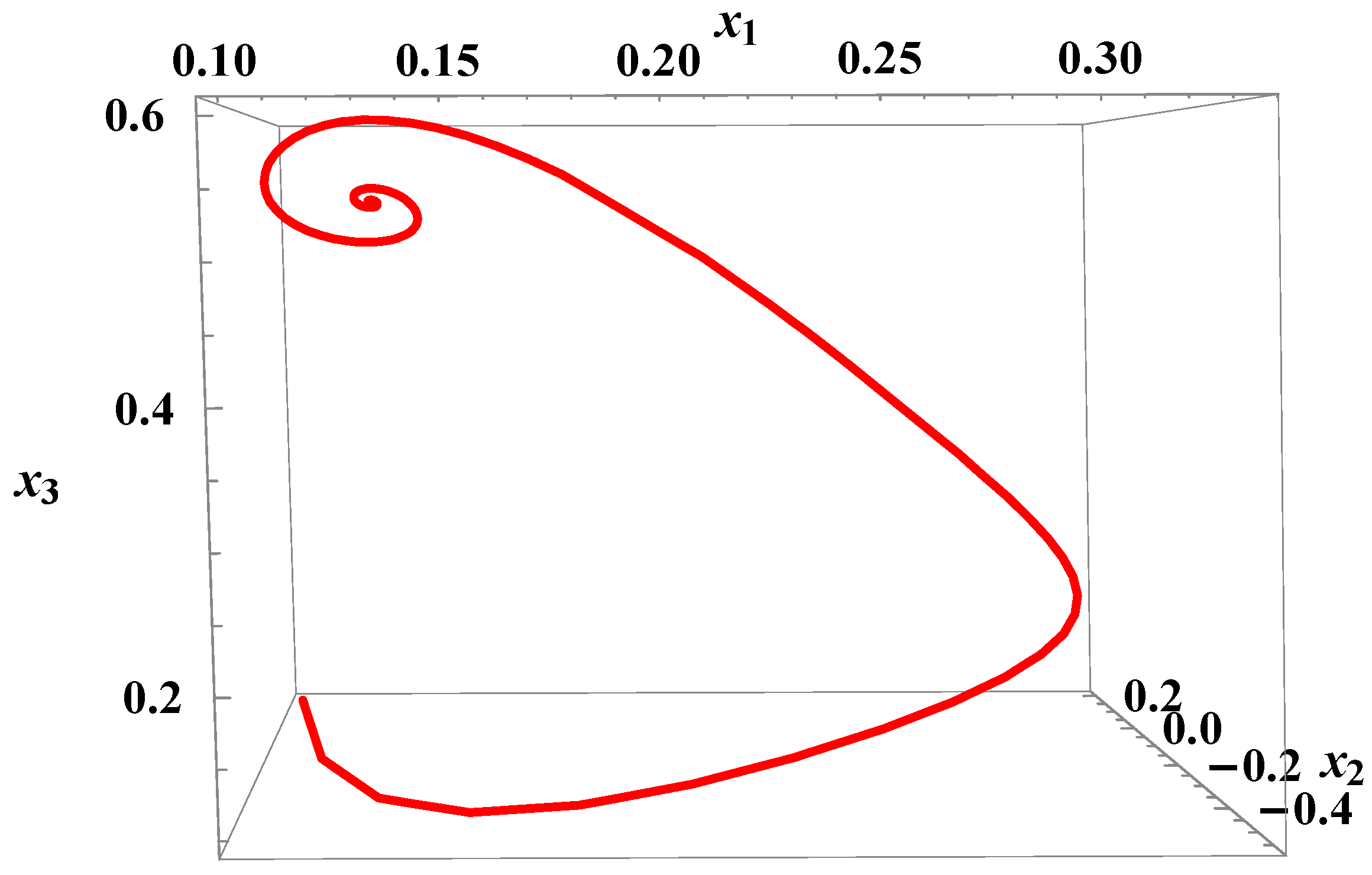
Lemma 1. For any , there exists an open set containing where the matrix has rank 3 and is involutive.
, for non-zero values of state variables involved in
. It is also confirmed by
Figure 1.
Therefore
or equal to the order of the system. With the help of Equations (7) and (8) one can show that:
which shows that
belongs to
. Hence,
S is involutive.
Lemma 2. For any thrice differentiable function , there exists, a smooth transformation with a smooth inverse, defined on an open set where that reduces Equation (6) to a linear controllable form.
Proof. Since Lemma 1 holds, there exists a real valued function
such that
and
but,
. Now,
implies
and
implies
. Hence
is independent of
and
but depends on
. Thus,
where simple calculations yield,
as
.
With the help Equation (11) one can easily calculate the following Lie derivatives given as
where,
,
,
.
With the help of Equation (12), the transformation Equation (3) takes the form
Inverse transformation can be calculated from Equation (13) as
Controller
u is obtained from the Equation (3) as
These will change the TDCM given by Equation (6) into a linear controllable system:
where
is considered linear in
, and
. Without loss of generality, one may choose the linear form of
as
where,
.
Theorem 1 [8]. (Stabilization at a point): The controller stabilizes the equilibrium point iff and .
Theorem 2 [8]. (Stabilization onto a limit cycle—Hopf bifurcation): The controller stabilizes the system on to a stable limit cycle if and .
Now, using Equations (12) and (15), the controller
u can be written as:
Equation (6) with an output function becomes a controlled one when the control loop is closed with control input given by Equation (17).
Now the problem is studied for the particular forms of . However, there are many choices for (i.e., linear, quadratic, etc. in ). Here we choose only linear because the other forms will give more complicated forms of u after tedious calculations.
Let, a linear output
will give control law:
stabilizes Equation (6) to the control goal
or
where
is the parameter that determines the control goal.
Let
, where
is arbitrary constant to be determined later. Controlling Equation (17) to the origin and changing the values of
, one can control
x to the control goal
. In this case control law takes the form:
for the transformations, from linear to nonlinear and
vice versa, we have the following relations respectively,
Similarly, using reverse transformation, someone can find
x in terms of
z. Below the same has been written using
Mathematica:
where
and
.
Since the feedback control law stabilizes the equilibrium point of Equation (16), then using Equation (21) and changing the value of
K, one can control
to the goal
and the variation of
K is given by the formula:
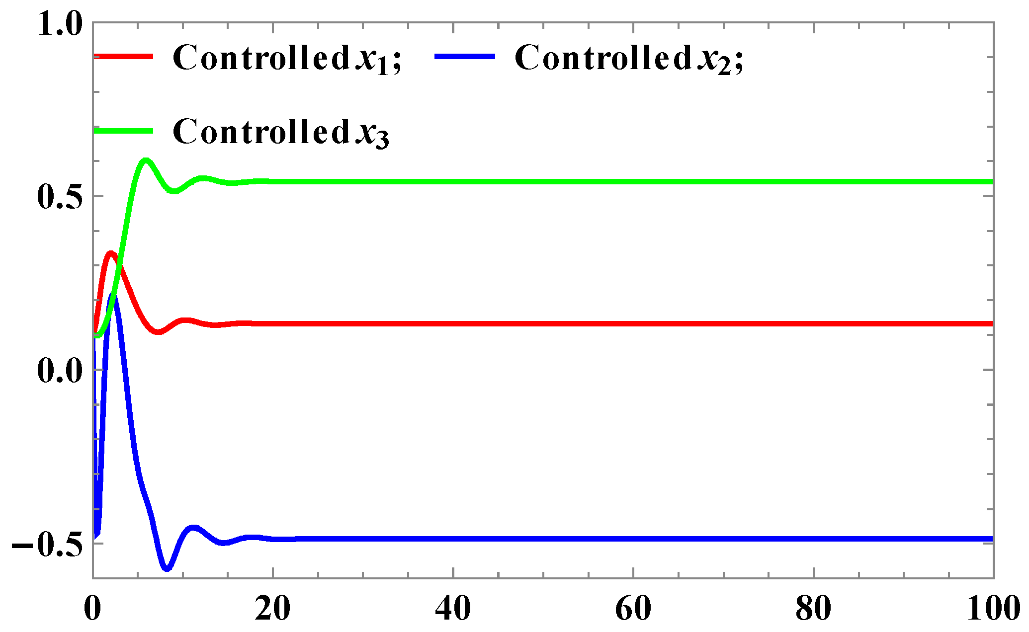
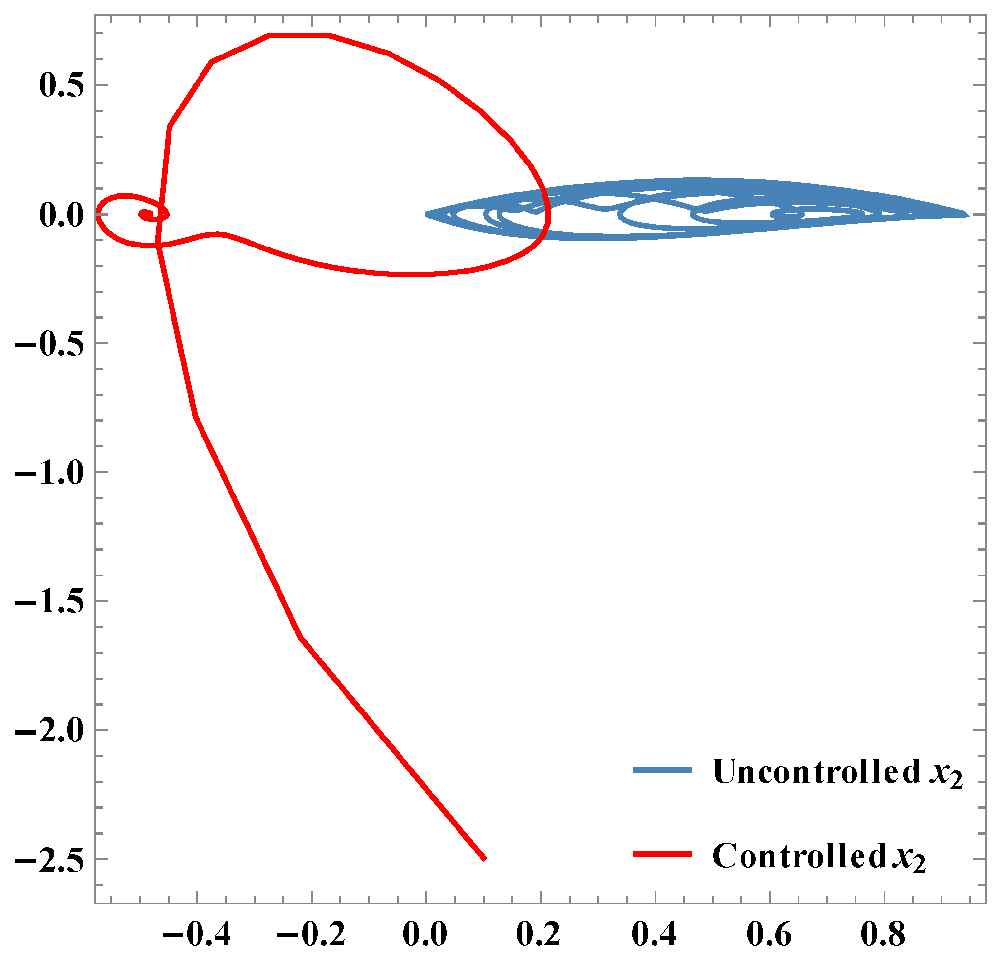
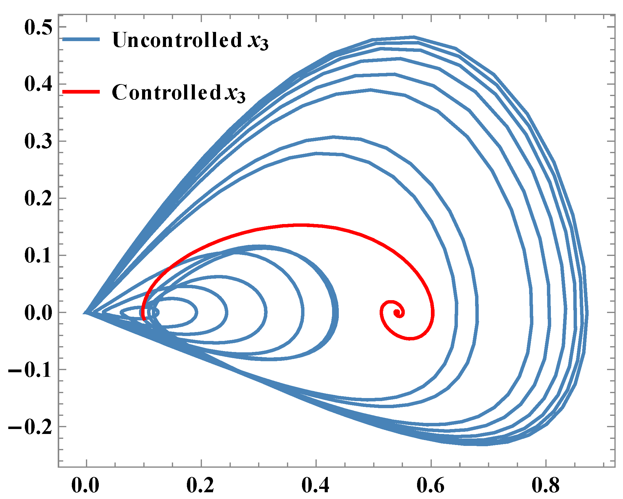
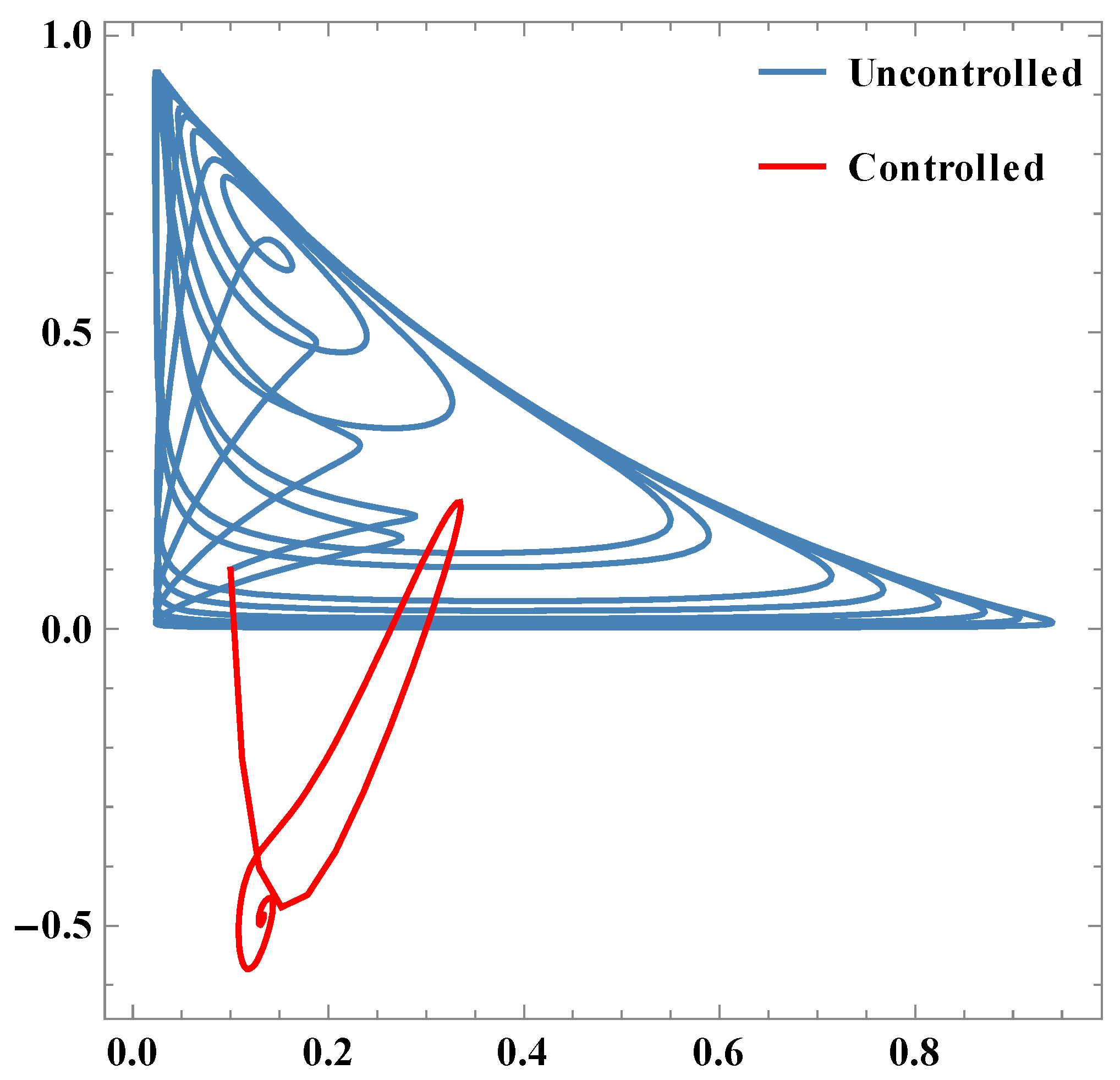
As x3 goes to the goal xg, the state vector x goes to or .


