Article

Sinc-Approximations of Fractional Operators: A Computing Approach

1
Mathematics Department, German University in Cairo, New Cairo City, 11835, Egypt
2
Mathematical Physics, University of Ulm, Ulm, D-89069, Germany
3
Mathematics, University of Utah, Salt Lake City, UT, 84112, USA
*
Author to whom correspondence should be addressed.
Mathematics 2015, 3(2), 444-480; https://doi.org/10.3390/math3020444
Submission received: 1 April 2015 / Accepted: 20 May 2015 / Published: 5 June 2015
(This article belongs to the Special Issue Recent Advances in Fractional Calculus and Its Applications)

Abstract

:
We discuss a new approach to represent fractional operators by Sinc approximation using convolution integrals. A spin off of the convolution representation is an effective inverse Laplace transform. Several examples demonstrate the application of the method to different practical problems.

1. Introduction

During the past 300 years a large number of fractional operators were used by researchers to overcome the Leibniz’s problem of fractional differentiation [1]. One of the contributors in this field was Abel with his famous integral equation [2]. The large numbers of novel applications of fractional differential equations in physics, chemistry, engineering, finance, and other sciences that have been developed in the last few decades created the demand to have numerical procedures to support the solution of these problems. In fact, the problem is that in all cases of fractional operators we must be able to deal with singular operators, and more specifically, with weak singular operators. In this paper we deal with only a few of these operators connected with their inventors Riemann, Liouville, Weyl, and Caputo [3]. Based on these integral operators we define fractional integral and differential equations which turn out again to be singular integral equations using a singular convolution kernel of Abel-type [3]. This type of singular kernels is the main obstacle of numerical methods in the field.
There are different approaches to overcome the problems with singularities. However, it turns out that most of the methods used to circumvent the problems are not effective. Standard methods for the numerical calculation of fractional integrals and derivatives are typically slow and memory consuming due to the non locality of the operators [48]. For example Lubich proposes a discrete convolution procedure based on a linear multistep method [9]. Yuan and Agrawal have proposed a more efficient approach based on Laguerre integral formulas for operators whose order is between 0 and 10. Their approach differs substantially from the traditional concepts [10,11]. However, the accuracy of the results can be poor. Diethelm modified the algorithm, adapting it to the properties of the problem, and demonstrated that this leads to a significantly improved quality [12]. However, both approaches use the same idea to convert the original problem to a system of first order initial value problems which seems to be an approach with a low convergent rate. In fact all the methods discussed in literature have polynomial convergence compare [8,13,14] and references therein.
In this paper we follow a new direction of approximation theory introduced by [15] in connection with convolution integrals [16]. The Sinc methods, e.g., [15,16] have among other features a very fast convergence of exponential order exp (−CN1/2) with C a positive constant and in addition converges even when the explicit nature of singularities is unknown. Popular numeric solvers, i.e., finite difference and finite elements, have severe limitations with regard to speed and accuracy, as well as intrinsic restrictions making them ill fit for realistic, less simplified problems. Spectral methods also have substantial difficulties regarding complexity of implementation and accuracy of solution in the presence of singularities. However, in the case when the nature of the singularity is known, then suitable boundary element bases can be selected to produce an approximation that converges rapidly. On the other hand, it is often difficult to deduce a priori the nature of the singularity, and in such cases methods based on polynomial or finite element approximations converge very slowly.
We will restrict our discussions to the practical application of the Sinc method to different fractional differential equations (FDE). We note however that, apart from the approach that we will use, several other numerical methods for treating integrals, derivatives, and solutions of differential equations of fractional order have been developed. The most prominent one—the decomposition method attributed to Adomian [17]—has rather poor convergence properties in general [18,19].
The variational iteration method is based on the use of restricted variations combined with correction functional and the Lagrange multiplier technique. The method rely on the knowledge of the Lagrange multiplier which for non-linear problems is not directly accessible [20,21]. The homotopy analysis method [22] and the homotopy perturbation method [20] are slow in convergence in connection with FDEs. The generalized differential transform method [23] and a few others deliver poor solutions and moreover, the convergence proofs given apply in very restrictive conditions [24]. There are many other methods known, which also do not converge satisfactorily [25]. This situation creates a demand for an effective method which is able to deal with singularities, which is highly accurate, and which converge rapidly.
The integrals we shall discuss in this paper are Riemann integrals which we assume to be locally and absolutely integrable on ℝ+. Let B = [a, b] with (−∞ < a < b < ∞) be a finite interval on the real axis ℝ. The Riemann-Liouville fractional integrals D a , x v and W x , b v of order v ∈ ℂ (e(v) > 0) are two typical examples of integrals we shall deal with
D a , x v u ( x ) = 1 Γ ( v ) a x ( x t ) v 1 u ( t ) d t , ( v ) > 0 ,
and with
W x , b v u ( x ) = 1 Γ ( v ) x b ( t x ) v 1 u ( t ) d t , ( v ) > 0 ,
where Γ(v) is the gamma function. In literature [3], these two integrals are commonly called left- and right-sided fractional integrals. The common feature of both types of integrals is that they represent convolution integrals using a singular kernel of the Able-type; i.e., t−μ with 0 < μ ≤ 1, as a typical example. Our aim in this paper will be the approximation of integral equations (IE) with such singular convolution operators.
The two integral operators D a , x v and W x , b v can be generalized to a non-linear version known as non-linear Volterra–Hammerstein integral equations of convolution type [7]
L ( u ( x ) ) = 0 x G ( x s ) K ( s , u ( s ) ) d s + g ( x ) and x ( a , b )
where L, K, g, and G are explicitly known continuous generic functions and where u is unknown. Note L might be linear or non-linear while K is a generic non-linear function. We shall in addition to Equations (1) and (2) also consider such equations of this paper.

2. Approximation Method

This section introduced the basic ideas of Sinc methods. We shall introduce some ideas of Sinc approximation relevant to our paper [26]. We omit most of the proofs of the different important theorems and lemmas because these proofs are available in literature [16,2931]. The following subsections collect information on the basic mathematical functions used in Sinc approximation. We introduce Sinc methods to represent indefinite integrations and convolution integrals. These types of integrals are essential for representing the fractional operators of differentiation and integration [29].

2.1. Sinc Bases

To start with we first introduce some definitions and theorems allowing us to specify the space of functions, domains, and arcs for a Sinc approximation.
Definition 1. Domain and Conditions.
Let D be a simply connected domain in the complex plane and z ∈ ℂ having a boundary D. Let a and b denote two distinct points of D and let φ denote a conformal map of D onto D d, where D d = { z : | I m ( z ) | < d }, such that φ(a) = −∞ and φ(b) = ∞. Let ѱ = φ1 denote the inverse conformal map, and let Γ be an arc defined by Γ = {z ∈ ℂ: z = ѱ (x), x ∈ ℝ}. Given φ, ѱ, and a positive number h, let us set zk = ѱ (kh), k ∈ ℤ to be the Sinc points, and let us also define ρ(z) = eφ(z).
In the calculations which follow we use the conformal maps φ(z) = log((z − a)/(b z)) and its inverse ѱ(z) = (b+a exp(z))/(1+exp(z)) for finite intervals (a, b). Other conformal maps for different arcs Γ can be found in [31]. Note Burchard and Höllig [32] prove that there is no method that converges faster than Sinc, for approximating functions that are analytic on the interior of an arc, but may have singularities of unknown type at the end points. This argument is supported by the recent findings on Lebesgue measures for Sinc approximations [33].
Definition 2. Function Space.
Let d ∈ (0, π), and let the domains D and D d be given as in Definition 1. If d′ is a number such that d′ > d, and if the function φ provides a conformal map of D onto D d , then D D . Let L α , β ( D ) be the set of all analytic functions, for which there exists a constant c1, such that
| u ( z ) | c 1 | ρ ( z ) | α ( 1 + | ρ ( z ) | ) α + β .
Now let the positive numbers α and β belong to (0, 1], and let M α , β ( D ) denote the family of all functions g Hol ( D ), such that g(a) and g(b) are finite numbers, where g(a) = limza g(z) and g(b) = limzb g(z), and such that u L α , β ( D ) where
u ( z ) = g ( z ) g ( a ) + ρ ( z ) g ( b ) 1 + ρ ( z ) .
The two definitions allow us to formulate the following theorem for Sinc approximations.
Theorem 1. Sinc Approximation [16].
Let u L α , β ( D ) for α > 0 and β > 0, take M = [βN/α], where [x] denotes the greatest integer in x, and then set m = M + N + 1. If u M α , β ( D ), and if h = (πd/(βN))1/2 then there exists a positive constant c2 independent of N, such that
| u ( z ) j = M N u ( z j ) w j | c 2 N 1 / 2 e ( π d β N ) 1 / 2 .
where wj denote the basis functions defined by
w j = { 1 1 + ρ ( z ) k = M + 1 N 1 1 + e k h S ( k , h ) φ ( z ) j = M S ( j , h ) φ ( z ) j = M + 1 , , N 1 ρ ( z ) 1 + ρ ( z ) k = M N 1 e k h 1 + e k h S ( k , h ) φ ( z ) j = N
with S(j, h) the shifted Sinc
S ( j , h ) φ ( z ) = S i n c ( [ φ ( z ) j h ] / h ) , j = M , , N .
based on the Sinc function
S i n c ( z ) = sin ( π z ) π z .
The proof of this theorem is given in [16]. Note the choice h = (πd/(βN))1/2 is close to optimal for an approximation in the space M α , β ( D ) in the sense that the error bound in Theorem 1 cannot be appreciably improved regardless of the basis [16]. It is also optimal in the sense of the Lebesgue measure achieving an optimal value less than Chebyshev approximations [33].
The discrete shifting in Equation (8) allows us to cover the approximation interval (a, b) in a dense way while the conformal map is used to map the interval of approximation from an infinite range of values to a finite or a semi-infinite one, or even to an analytic arc.
A Sinc approximation is then defined as follows. Select positive integers N and M = [βN/α] so that m = M + N + 1. The step length is determined by h = (πd/(βN))1/2 where α, β, and d are real parameters. In addition assume there is a conformal map φ and its inverse ѱ such that we can define Sinc points zj = ѱ (jh), j ∈ ℤ [16]. This allows us to define a row vector w m T of basis functions
w m T = ( w M , , w N ) = ( w M w N ) T
with wj defined as in Equation (7). For a given vector V m(u) = (u−M,…, uN)T which maps a function u = u(x) to its discrete values uk = u(zk). The superscript “T” here and in the following denotes the transpose. We now introduce the dot product as an approximation of the function u by
u w m T V m ( u ) = k = M N u k w k .
If it is obvious from the context, we also will use the notation where the subscripts m are dropped, i.e., dot products, when there is no misunderstanding. Based on this notation, we will introduce the different integrals we shall require in the next few subsections [29].

2.2. Indefinite Integral

As a basis for the representation of fractional derivatives, we need indefinite integrals. This subsection describes how indefinite integrals can be defined [16] and how these definitions are related to the definition of definite integrals. Let us now discuss the collocation of the integrals J + and J defined by
( J + u ) ( x ) = a x u ( t ) d t with x ( a , b ) ,
( J u ) ( x ) = x b u ( t ) d t with x ( a , b ) .
Let ℤ denote the set of all integers, and let ℂ denote the complex plane. Let Sinc(z) be given by Equation (9) and let ek be defined as
e k = 1 2 + σ k , k ,
with
σ k = 0 k Sinc ( x ) d x = 1 π Si ( π k )
and Si ( x ) = 0 x t 1 sin ( t ) d t the sine integral.
If now φ denotes a one-to-one transformation of the interval (a, b) onto the real line ℝ as defined above, then let h denote a fixed positive step length, and let the Sinc points be defined on (a, b) by zk = φ1(kh), k ∈ ℤ, where φ1 denotes the inverse function of the conformal map φ. Let M and N be positive integers, set m = M + N + 1, and for a given function u defined on (a, b), define a diagonal matrix D(u) by D(u) = diag [u (z−M),…, u (zN)]. Let I(−1) be a square Töplitz matrix of order m having ei−j, as its (i, j)th entry, and, i j = −M,…,N, then
( I ( 1 ) ) i , j = e i j with , i , j = M , , N .
Define square matrices A m + and A m by
A m + = h I ( 1 ) D ( 1 / φ ) = A +
A m = h ( I ( 1 ) ) T D ( 1 / φ ) = A .
The collocated representation of the indefinite integrals are thus given by
J m ± u = w T A ± V ( u ) .
These are collocated representations of the indefinite integrals defined in Equations (12) and (13), respectively [29]. Quite recently it was proved that the eigenvalues of the matrix I(1) lie in the open right half-plane [37]. Note the matrices A m ± arises in several applications of Sinc methods and have positive eigenvalues on the open right half-plane [29]. The matrices ( ± A m ± ) 1 yield accurate approximation of derivatives, i.e., their inverses exist, since the real parts of their eigenvalues are on the open right half plane, and so
u ( ± A ± ) 1 V ( u ) .
Comparing our results with the target equations for example Equations (1) and (2), we observe that we need one additional step to extend the indefinite integrals to convolution integrals.

2.3. Convolution Integrals

Indefinite convolution integrals can also be effectively collocated via Sinc methods [16]. This section discusses the core procedure of this paper, for collocating the convolution integrals and for obtaining explicit approximations of the functions p and q defined by
p ( x ) = a x f ( x t ) g ( t ) d t with x ( a , b ) ,
and
q ( x ) = x b f ( t x ) g ( t ) d t with x ( a , b ) ,
where x ∈ Γ. In presenting these convolution results, we shall assume that Γ = (a, b) ⊆ ℝ, unless otherwise indicated. Note also, that being able to collocate p and q enables us to collocate definite convolutions like a b f ( x t ) g ( t ) d t. Recently such convolution integrals were determined by accurate tensor approximation [27,28].
Before we start to present the collocation of the Equations (21) and (22), we mention that there is a special approach to evaluate the convolution integrals by using a Laplace transform. Lubich [6,7] introduced this way of calculation by the following idea
p ( x ) = 0 x f ( x t ) g ( t ) d t = 1 2 π i c F ( s ) 0 x e s t g ( x t ) d t d s
for which the inner integral solves the initial value problem y′ = sy + g with g(0) = 0. The Laplace transform
F ( s ) = E f ( t ) e t / s d t
with E any subset of ℝ such that E ⊇ (0, b − a), exists for all s ∈ Ω+ = {s ∈ ℂ | ℜ(s) > 0}. Furthermore, if the Laplace transform Equation (24) exists for all ℜ(s) > 0, then F ( A m ± ) are well defined.
In view of Equation (19), we can expect that the approximations
p = F ( J + ) g F ( J m + ) g ,
and
q = F ( J ) g F ( J m ) g ,
are also accurate, which is, in fact, the case [29]. The procedure to calculate the convolution integrals is now as follows. The collocated integrals take the form J ± = w m T A m ± V m, where
A m ± = X m ± diag [ s m , M , , s m , N ] ( X m ± ) 1 ,
and with Σ = diag [s−M,…, sN] the diagonal matrix for each of the matrices A m ±. Then the Laplace transform Equation (24) delivers the square matrices F ( A m ± ) defined via the equations
F ( A m ± ) = X m ± diag [ F ( s m , M ) , , F ( s m , N ) ] ( X m ± ) 1 = X m ± F ( ) ( X m ± ) 1 .
We can then get the approximation of Equations (25) and (26) from the expression
F ( J ± ) g F ( J m ± ) g = w T F ( A ± ) V ( g ) .
These two formulas enable us to obtain vectors whose entries approximate p and q at the Sinc points. The convergence of the method is exponential as was proved in [16].
For the non-linear case of convolution with the target to represent Equation (3), we state the following result, taken from [31]:
Theorem 2. Non-linear Convolution.
Let D = D ( a , b ) be defined as in Definition 1, and let L α , β ( D ) be defined as in Definition 2. Assume that K(·, c) is analytic and uniformly bounded in D ( a , b ) for each c ∈ [c1, c2] and also, that K(x, ·) is analytic and uniformly bounded in D ( c 1 , c 2 ) for each fixed x ∈ (a, b). If u L α , β ( D ), and if P is defined by
P ( x ) = 0 x G ( x t ) K ( t , u ( t ) ) d t , w i t h x ( a , b ) ,
then PLα,β. In the above notation, with F denoting the Laplace transform of G, we write
P = F ( J ) K ,
i.e.,
V m ( P ) = F ( A m + ) V m ( K )
with Vm(K) = (K (z−M, u (z−M)), K (z−M+1, u (z−M+1))…, K (zN, u (zN)))T. Let M = N and h = (πd/(αN))1/2, then there exists a constant c3 which is independent of N such that
E ( G , K ) = | P w T { F ( A + ) V ( K ) } | c 3 N 1 / 2 e ( π d α N ) 1 / 2
and wT as defined in Equation (10). A similar formulation can be given for Q ( x ) = x G ( t x ) K ( t , u ( t ) ) d t.
The proof of this theorem can be found in [31]. The use of Theorem 2 allows us to write for the non-linear convolution integral an approximation at Sinc points xk as follows
0 x k G ( x k s ) K ( s , u ( s ) ) d s = j = N N F k j K ( x j , u ( x j ) ) + E k ( G , K ) , k = N , , N ,
where Fkj is the (k, j) entry of matrix F ( A m + ) and the error at a certain Sinc point xk satisfies Ek(G, K) ≤ E(G, K). Equation (34) will be useful later on to estimate the error in a non-linear problem (see Theorem 8).

3. Sinc Representation of Fractional Operators

This section presents the main operators which are frequently used in practical problems. We present the basic notations first and then use them in collocated approximations. The collocation formulas have a common structure for linear operators. The non-linear version only deviates in the generic function K but also allows a separation of spectral and discrete properties of the operators.

3.1. Fractional Integrals

The Riemann-Liouville fractional integrals Equations (1) and (2) defined on the finite interval (a, b) of the real line ℝ, are naturally extended to the half-line ℝ+. The two integrals for the positive real line have corresponding to the representation of Miller and Ross [38] the forms:
D 0 , x v u ( x ) = 1 Γ ( v ) 0 x ( x t ) v 1 u ( t ) d t , ( v ) > 0 ,
and
W x , v u ( x ) = 1 Γ ( v ) x ( t x ) v 1 u ( t ) d t , ( v ) > 0.
Both integrals are of convolution type. We shall describe below the approximation of these integrals by use of our convolution Sinc methods.

3.2. Fractional Derivatives

Let n ∈ ℕ be the smallest natural number greater than ℜ(μ), and let v = n – μ, then 0 < ℜ(v) ≤ 1. Here ℕ denotes the set of natural numbers. The Riemann-Liouville fractional derivatives on the real line D a , x μ and W x , b μ of order μ with μ ∈ ℂ and ℜ(μ) ≥ 0 are defined by
D a , x μ f ( x ) = d n d x n [ D a , x v u ( x ) ] = D a , x n [ D a , x v u ( x ) ] ,
and
W x , b μ u ( x ) = d n d x n [ W x , b v u ( x ) ] = W x , b n [ W x , b v u ( x ) ] ,
These two definitions use Riemann-Liouville integrals to represent the derivatives. We again omit the straight forward extensions of the integrals Equations (37) and (38) to ℝ+—see [3].
In some of the applications it is important to incorporate the initial conditions into the fractional derivative. For such cases another type of fractional derivatives was introduced by Caputo [34]. Kilbas et al. define these types of derivatives as follows
D c μ a , x u ( x ) = 1 Γ ( n μ ) a x ( x t ) n μ 1 u ( n ) ( t ) d t , x > a , ( μ ) > 0 , n = [ ( μ ) ] + 1 ,
and
W c μ x , b u ( x ) = 1 Γ ( n μ ) x b ( t x ) n μ 1 u ( n ) ( t ) d t , x < b , ( μ ) > 0 , n = [ ( μ ) ] + 1.
The difference between the Riemann-Liouville and the Caputo derivative is that the integer order derivative is applied to the integrand of the integral. The Caputo derivative has proven to be an important tool in mathematical modeling of many phenomena in physics and engineering, see, e.g., [13,14,35] and the references therein.

3.3. Fractional Integral Equations

In this section we consider converting an fractional integral equation (FDI) to an integral equation (IE). Consider, for example, the simple Riemann-Liouville equation,
u ( x ) D 0 , x v u ( x ) = g ( x ) .
Using Equation (35), this equation can also be written in the form
u ( x ) 1 Γ ( v ) a x ( x t ) v 1 u ( t ) d t = g ( x ) ,
which is just a linear Volterra equation of the form
u ( x ) a x G ( x , t ) u ( t ) d t = g ( x ) ,
with G(x, t) = (x − t)v−1/Γ(v). A generalization to non-linear FIE is straight forward if we replace in Equation (41) the term D 0 , x v u ( x ) with a generic non-linear function K in D 0 , x v K ( x , u ( x ) )
u ( x ) D 0 , x v K ( x , u ( x ) ) = g ( x ) ,
which is just
u ( x ) a x G ( x , t ) K ( t , u ( t ) ) d t = g ( x ) .
The integral Equation (45) is a Volterra integral equation which is also known as Hammerstein’s equation.

3.4. Fractional Differential Equations

Next let us discuss the formulation of linear fractional differential equation using the Riemann-Liouville fractional derivative D a , x μ u ( x ) of order μ > 0 in a Banach space of continuous functions [3]. The Cauchy type problem for the fractional differential equation of order μ > 0 is given by
D a , x μ u ( x ) λ u ( x ) = g ( x ) , with a < x b , μ > 0 and λ ,
and with the initial conditions
D a , x μ k u ( x ) | x = a = b k with b k , k = 1 , , n = μ ,
where ⌈μ⌉ denotes the smallest integer greater than ℜ(μ), and where we assume that gCγ[a, b], with Cγ[a, b] denoting the weighted space of continuous functions and 0 ≤ γ < 1 is equivalent to the solution to the initial value problem Equations (46)(47) is thus given by The proof that Equation (48) is solution of Equations (46) and (47) is given by
u ( x ) λ Γ ( μ ) a x ( x t ) μ 1 u ( t ) d t = 1 Γ ( μ ) a x ( x t ) μ 1 g ( t ) d t + j = 1 n b j Γ ( μ j + 1 ) ( x a ) μ j
The proof that Equation (48) is solution of Equations (46) and (47) is given by Kilbas et al. [3].
The formulation of the Cauchy type initial value problem using the Caputo fractional derivative D c v a , x u ( x ) for μ > 0 and μ ∉ ℕ can be formulated in a similar way for such a simple equation as
D c μ a , x u ( x ) λ u ( x ) = g ( x ) with a x b , n 1 < μ < n , n , and λ ,
with initial conditions
u ( k ) ( x ) | x = a = b k with b k , k = 0 , , n 1.
This problem again is equivalent to the solution of a Volterra integral equation of the second kind as shown in [3]
u ( x ) λ Γ ( μ ) a x ( x t ) μ 1 u ( t ) d t = 1 Γ ( μ ) a x ( x t ) μ 1 g ( t ) d t + j = 0 n 1 b j Γ ( j + 1 ) ( x a ) j .
The two types of fractional differential equations have the nice property that their solution is represented by convolution integrals. Such integrals can be easily dealt with our indefinite convolution and Sinc approximation procedures. Although we know the solutions Equations (48) and (51) of the FDEs Equations (46) and (49), we still have to solve a Volterra integral equation of the second kind. In the next section we shall describe our method of obtaining this solution.
Problems exist in applications which contain both fractional and ordinary derivatives [37]. Such problems can also be readily dealt with using our methods.
So far we discussed only linear fractional differential equations. However, in some of the applications non-linear models are used [8]. Another example of non-linear fractional differential equation was examined in [42,43]. Diethelm discusses the numerical algorithm for the following fractional equation
D c μ 0 , x u ( x ) = g ( x , u ( x ) ) with μ > 0 and n 1 < μ < n , n ,
combined with initial conditions
u ( k ) ( 0 ) = u 0 ( k ) and k = 0 , 1 , , n 1.
This initial value problem is equivalent to the Volterra integral Equation, [43]
u ( x ) 1 Γ ( μ ) 0 x ( x t ) μ 1 g ( t , u ( t ) ) d t = j = 0 n 1 u 0 ( j ) Γ ( j + 1 ) x j .
A generalization of this equation to a system of equations is given by Daftardar [39]. Again we end up with a Volterra integral equation which uses an integral of convolution type. As we already discussed above, the convolution property is very useful in dealing with numerical solutions of these equations. All the FIEs and FDEs discussed so far are treated in literature with “standard” methods. The results gained by these approaches are limited to a certain accuracy combined with a high demand of computational efforts. In the following we will show how the accuracy can be improved and the computational tasks reduced to a minimum.
Let us introduce the discrete Sinc representation of integral equations of the different types discussed above. Using Equations (21) and (22) as basis, we know how to collocate convolution integrals in Volterra integral equations of second kind by applying Sinc methods.

3.5. Collocation of Fractional Integral Equations

Concerning the discrete representation of the Volterra integral Equations (41) and (43) we have the approximation
u F ( J ) u = g { I F ( A + ) } V ( u ) = V ( g ) .
The non-linear version of the FIE Equations (44) and (45) has the collocated representation
u F ( J ) K ( u ) = g { I F ( A + ) } V ( u ) = V ( g ) .
The solutions in both cases follows by
u ( x ) w T V ( u ) .
In the first case we have to solve a linear system of equations while the second case needs the solution of a non-linear system of equations. Which in both cases can be numerically achieved by Newton’s method and Newton-Kantorovich iteration.

3.6. Collocation of Fractional Differential Equations
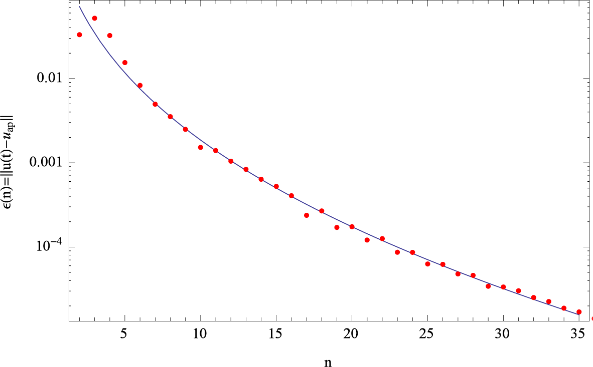
For fractional differential equations there exists a solution in terms of a second kind Volterra integral equation incorporating the initial conditions of the Cauchy problem as given in Equations (46) and (47). The discrete version of these equations ensue by collocating Equation (48) as follows:
u λ F ( J ) u = F ( J ) g + N V ( u ) λ F ( A + ) V ( u ) = F ( A + ) V ( g ) + V ( N ) .
N collects initial conditions of the problem. The discrete version follows straight forward from Equation (58) to be
{ I λ F ( A + ) } V ( u ) = F ( A + ) V ( g ) + j = 0 n = 1 b j Γ ( μ j + 1 ) V ( ( x α ) μ j ) .
Caputo’s fractional differential Equation (51) allows the solution in a collocated Sinc representation as
u λ F ( J ) u = F ( J ) g + N V ( u ) λ F ( A + ) V ( u ) = F ( A + ) V ( g ) + V ( N ) .
N collects initial conditions of the problem. The discrete version follows from Equation (60) to be
{ I λ F ( A + ) } V ( u ) = F ( A + ) V ( g ) + j = 0 n 1 b j Γ ( j + 1 ) V ( ( x α ) j ) .
Solving this linear system in both cases with respect to V (u) allows us to approximate the solution by
u ( x ) w T V ( u ) .
For the non-linear singular Volterra equation we can derive the determining equations based on Theorem 2. Taking into account the exponential decay of the error E(G, K) we can write Equation (3) in its discrete form as
L ( V ( u ) ) F ( A + ) V ( K ( u ) ) = j = 0 n 1 u 0 ( j ) Γ ( j + 1 ) V ( ( x ) j ) .
This non-linear system of Equation (63) delivers the unknowns V (u) by applying Newton’s method and Newton–Kantorovich iteration method. The resulting approximation then enables us to represent the solution via Sinc approximation in the form
u ( x ) w T V ( u ) .
Let us next proof the convergence of the non-linear integral Equation (3). Let D and L be defined as above, corresponding to an interval (a,b). Let ν ϵ (0, 1], and let B denote the Banach space L = L.
We wish to consider proving the existence of a solution to the IE
u ( x ) 1 Γ ( ν ) a x ( x t ) ν 1 K ( t , u ( t ) ) d t = g ( x ) , x ( a , b ) .
Assumption 3. Let us assume that corresponding to some interval (C, D) to be made more specific below, that K(·, c) is analytic and uniformly bounded for all c ϵ (C, D), that K(x, ·) is analytic and informally bounded in D, and also that g ϵ L.
Let J + be defined on (a, b) as above, so that we can write the IE Equation (65) in the operator form
u J ν K ( , u ) = g ,
where we have used the simpler notation J for J +.
Lemma 4. If u is real–valued on (a,b), if u ϵ (C, D), and if u ϵ B , then J ν K(·, u) ϵ B.
Proof. Note to begin with, that since ν ∈ (0, 1], and since the eigenvalues of J + have non negative real parts and are located either on the real line or occur in conjugate pairs on the right half plane, the same is true for the eigenvalues of the operator. The proof then follows by inspection. □
Lemma 5. Let the conditions of Lemma 4 be satisfied. If | ( J + ) ν K ( · , u ) | < 1 for all u ∈ (C, D), then Equation (66) has a unique solution.
Remark 1. For a finite interval (a, b), we have for uBν, that
| ( J ν u ) ( x ) | 1 Γ ( ν ) sup t ( a , x ) | u ( t ) | a x ( x t ) ν 1 d t = x ν Γ ( ν + 1 ) | | u | | ( b a ) ν Γ ( ν + 1 ) | | u | | .
It thus follows from Remark 1 that the operator J ν K ( · , · ) is a contraction mapping for all |ba| sufficiently small, implying the statement of Lemma 5.
Assumption 6. Let (x, y) ∈ (a, b) × (C, D), let us assume that 0 ∈ (C, D), let us set
P ( x , y ) = K ( x , y ) K ( x , 0 ) y ,
and let us assume that Ky (x, y) ≤ c < 0 on (x, y) ∈ (a, b) (C, D), and that Ky (x, y) either is increasing or decreasing on (a, b) × (C, D). Set
u 0 ( x ) = g ( x ) + ( J ν K ( , 0 ) ) ( x ) .
Theorem 7. If Assumption 6 is satisfied, then the sequence { u n } n = 0 starting with u as in Equation (69) and
u n + 1 = T n u 0 ,
With
T n = ( I 1 Γ ( ν ) J ν P ( , u n ) )
converges to the unique solution on (a, b) × (C, D) of Equation (66).
Proof. Part 1. We consider first the case when P (x, ·) is decreasing on (C, D). We also assume at the outset that u0 (x) > 0 on (a, b). It then follows, since u0 > 0, that u 0 = ( T 0 ) 1 u 0 < u 0.
Next, we have, with Qn = ITn, that
u n + 1 u n = ( I Q n ) 1 ( Q n 1 Q n ) ( I Q n 1 ) 1 u 0 .
Since P is decreasing on (a, b), we have Q0Q1 < 0, and since u0 > 0, we have u1u2 < 0 on (a, b). It then follows by induction, that unun−1 < 0, i.e., that the sequence { u n } n = 0 is a positive, and decreasing sequence. This sequence must therefore have a unique limit.
The above argument also holds in the case when u0 is negative, or has sign changes on (a, b); in this case we simply replace the equal sign in Equation (72) by an inequality.
Part 2. Consider now the case when P (x, ·) is decreasing on (C, D). Once again assuming that u0 (x) > 0 on (a, b), we have u = (T0)−1 u0 < u0. Next, with the same definitions as in the above Part 1 proof, we now have Q0Q1 > 0, implying that u1 > u2. It thus follows from Equation (72) that we now get a nested sequence
u 1 < u 3 < < u 2 n 1 < u 2 n < u 2 n 2 < < u 0 .
That is we again get convergence to a unique solution. This same argument again holds in the case when u0 is negative, or when it changes sign on (a, b); by replacing the equal sign in Equation (72) with an inequality we then just get a monotonically convergent sequence of positive numbers, as we did in Part 1 of the proof.
Remark 2. We expect Theorem 7 to hold only under the assumption that ∂K(x, ·)/∂y is strictly negative on (a, b). One can imagine in such a case, the occurrence of a periodic, non-convergent sequence { u n } n = 0 , but this is doubtful under our analytic assumptions on K. This is particularly the case when we are using the approximating operators J m ±, since the eigenvalues of the indefinite integration matrices of these approximating operators have strictly positive real parts.
To analyze the error of the approximation Equation (64), we assume on the involved functions L, G, and K to be analytic. Then the following Theorem delivers an estimate of the error.
Theorem 8. Non-linear Volterra Equation.
Let us assume that the functions g, L, G, and K are analytic and satisfy the assumptions of Theorem 2, and let uk, k = −N,…, N denote the solutions to the approximating Equation (63). Then there exists a constant c4 that is independent of N, such that
max N k N | u ( x k ) u k | c 4 { 1 | F ( A m + ) | } 1 N 1 / 2 e ( π d α N ) 1 / 2 .
Proof. To start with the proof for the error we substitute Equation (34) in Equation (3) to obtain
L ( u ( x k ) ) j = N N u k j K ( x j , u ( x j ) ) = g ( x k ) + E k ( G , K ) , k = N , , N ,
and inserting the approximations given by Equation (64) into Equation (75), we get
L ( u ( x k ) ) L ( u k ) j = N N u k j { K ( x j , u ( x j ) ) K ( x j , u j ) } = E k ( G , K ) , k = N , , N .
Using now continuity of L, we write for the local error at Sinc points
| k | = | u ( x k ) u k | | L ( u ( x k ) ) L ( u k ) | = | j = N N u k j { K ( x j , u ( x j ) ) K ( x j , u j ) } + E k ( G , K ) | j = N N | u k j | | { K ( x j , u ( x j ) ) K ( x j , u j ) } | + | E k ( G , K ) | j = N N | u k j | | j | + | K k ( G , K ) | , k = N , , N .
Introducing the maximal error by = max N k N | k |, then
j = N N | u k j | + | E k ( G , K ) | max N k N j = N N | u k j | + max N k N | E k ( G , K ) | | F ( A m + ) | + E ( G , K ) .
This means
| F ( A m + ) | + E ( G , K ) ,
or
{ 1 | F ( A m + ) | } E ( G , K ) .
The final step of the proof is based on the spectral properties of F ( A m + ). The proof of the error formula becomes valid if we show that the spectral radius of any matrix A satisfies r σ ( A ) = max λ σ ( A ) | λ | < 1 with σ(A) the spectrum of A.
For the general interval (a, b) the following holds A+ = (h/φ′) I(−1), we have with x = φ(t), that (h/φ′)(t) = h(ba)ex/(1 + ex)2h(ba)/4, showing that the norm of A+ is proportional to the length of the interval ba, which allows the estimation
| | A + | | | | I ( 1 ) | | s u p x ( h e x ( 1 + e x ) 2 ( b a ) ) | | I ( 1 ) | | h 4 ( b a ) .
We have ample evidence from numerical computations that the spectral radius condition is satisfied for A m + and F ( A m + ) on a standard interval (a, b) = (0, 1).
Numerical calculations and Equation (81) suggest the decay r σ ( A m + ) = λ 1 / N with N = 1 , 2 , , where λ1 is the largest eigenvalue of σ ( A m + ). The value λ1 can be determined by direct computation using the smallest matrix A m + ; i . e . , N = 1. The value for the spectral radius is bound by r σ ( A m + ) < 1 / 3 and the analytic computation using the smallest matrix delivers r σ ( A m + ) 0.33227 … which is close to the given upper numerical bound.
The decay of the spectral radius r σ ( F ( A m + ) ) λ 1 , v N v / 2 and λ1,v = exp(−v) for v > 0. Again the relations hold for a standard interval (a, b) = (0, 1). The important point here is that the spectral radius for both matrices A m + and F ( A m + ) are smaller than 1: In this case the Neumann Lemma can be applied with | A m + | < 1 and | F ( A m + ) | < 1 the inverse of the relations ( 1 A m + ) 1 and ( 1 F ( A m + ) ) 1 exists and satisfies ( 1 A m + ) 1 1 / ( 1 A m + ) as well as ( 1 F ( A m + ) ) 1 1 / ( 1 F ( A m + ) ) and thus the error formula holds. Thus finally we get
c 4 1 | F ( A m + ) | N 1 / 2 e ( π d α N ) 1 / 2
with c4 a positive constant independent of N. Even more, since the spectral radii of both matrices are less than 1, successive iterations of the non-linear equation will converge to a fixed point according to the fixed point Theorem. This concludes the proof.
The result is that even for non-linear Volterra-Hammerstein integral equations the error in a Sinc approximation decays exponentially.
The different formulas presented in this section show that a Sinc approximation is basically derived from a collocation of the integral equations. The numeric steps of all of the calculations are straight forward and do not need any specialized numerical procedure. The core of the method is contained in the use of Sinc functions as a basis in connection with conformal maps. The formulas also show that an implementation uses standard objects like vectors and matrices which are simple to handle in any kind of programming language. However, since the method involves some symbolic steps we decided to do the implementation in Mathematica. A purely numeric implementation of Sinc methods in Matlab is provided by [29].

4. Examples

The examples presented in this section use implemented functions identifying the integral type used; e.g., RiemannLiouville and the type of the equation. I stands for integral equation FIE for fractional integral equation, NonlinearFIE[] for the non-linear version, etc. We implemented a set of functions using the discrete representation discussed in Section 3. In the following we will apply these functions to different problems and derive the related approximation of the solution. We start with simple applications like differentiation and integration, then solve linear integral equations, and finally deal with non-linear problems.

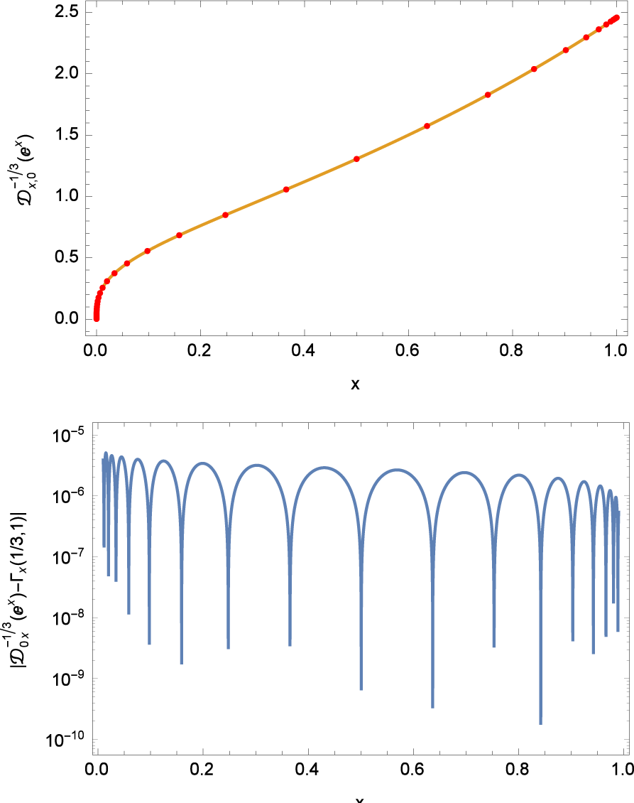
4.1. Generalized Gamma Function

In applications of fractional calculus it turned out that the generalization of the gamma function takes a prominent role [3,44,46]. The frequent occurrence of this function asked for an effective way to generate its numerical values. The difficulty of the generalized gamma function is that for arguments x → 0 the functions possesses a singularity which causes numerical problems. One possible approach to deal with such a problem is to generate the generalized gamma function applying Sinc methods to the corresponding Riemann-Liouville integral of order v
D 0 , x v e a x = x v e a x γ * ( v , a x ) = Γ x ( v , a ) .
The practical calculation is carried out by first defining in Mathematica the exponential function as
f ( x _ , a _ ) : = e a x
which is related to the generalized gamma function after integrating by the following relation
EE ( x _ , v _ , a _ ) : = e a x x v Γ ( v , 0 , a x ) Γ ( v ) ( a x ) v
The actual numerical integration of the exponential is performed by our Mathematica function RiemannLiouvilleI[] using f, the order v = 1/3, and N = 32 the number of Sinc points on an interval x ∈ (0, 1). The results of this integration for a specific choice of a = 1 is shown in Figure 1. In addition to the graph of the resulting function, we also plotted the location of the Sinc points. The distribution of the Sinc points gives us an idea how the discrete arrangement of the mesh along the x-axis is generated. The lower part of Figure 1 shows the local error of the approximation. We compare here our numeric results with the symbolic implementation of Ex(a,v) in Mathematica.
sol = RiemannLiouvilleI [ f [ x , 1 ] , x , 1 / 3 , 32 , 0 , 1 , 1 , 0 ] ;
The results displayed in Figure 1 show that the function possesses a vertical tangent if x → 0 causing numerical problems which need special treatments in “standard” approaches. In our calculations we do not need to care about such singularities at the end points because Sinc methods are able to deal with such behavior as an inherent property.

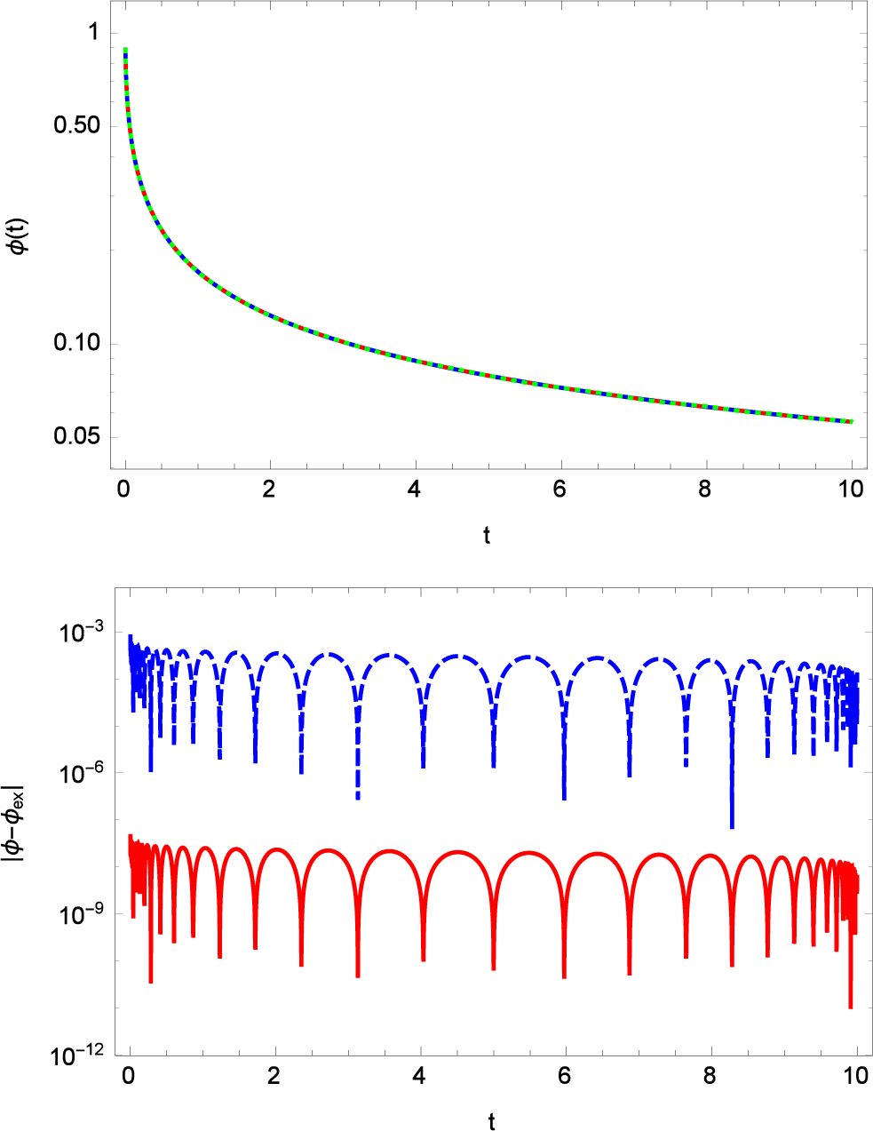
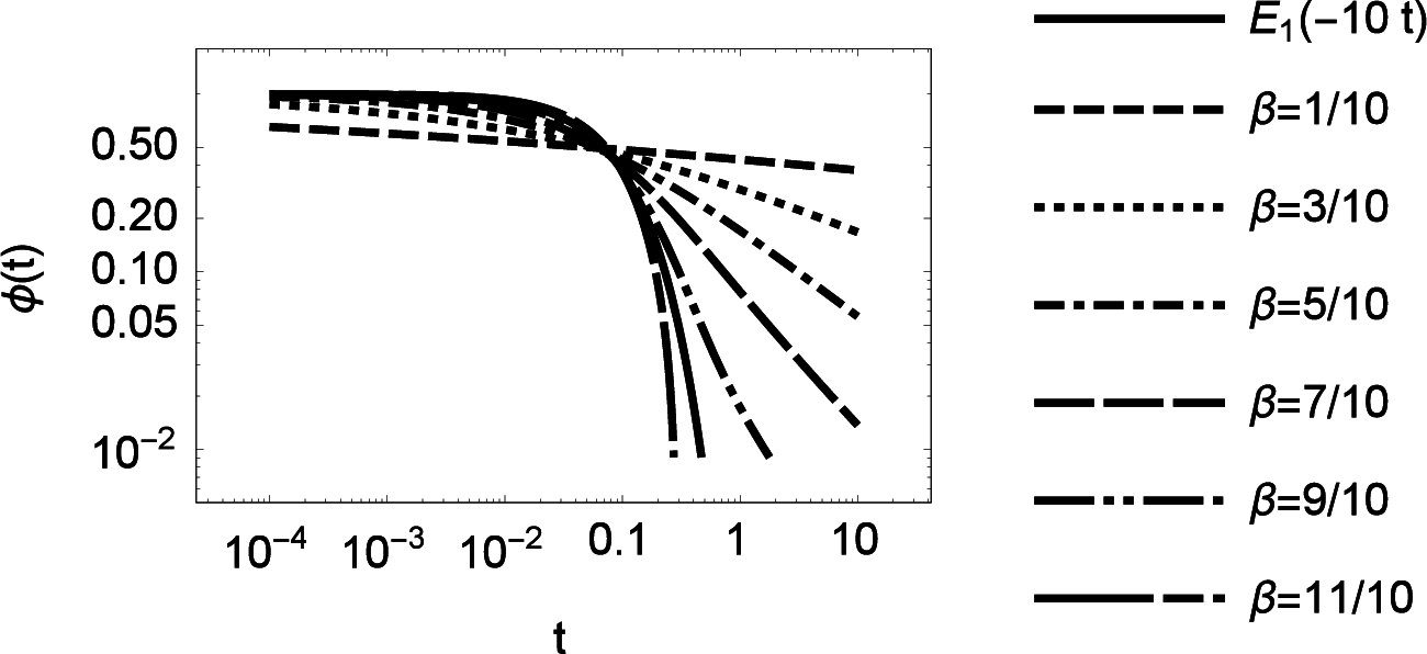
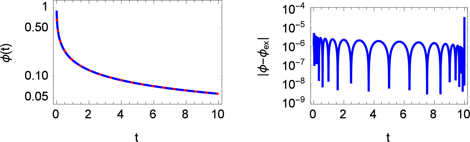
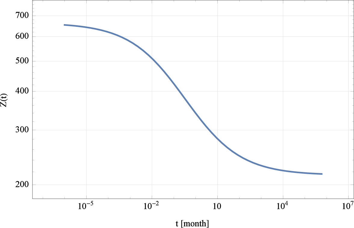
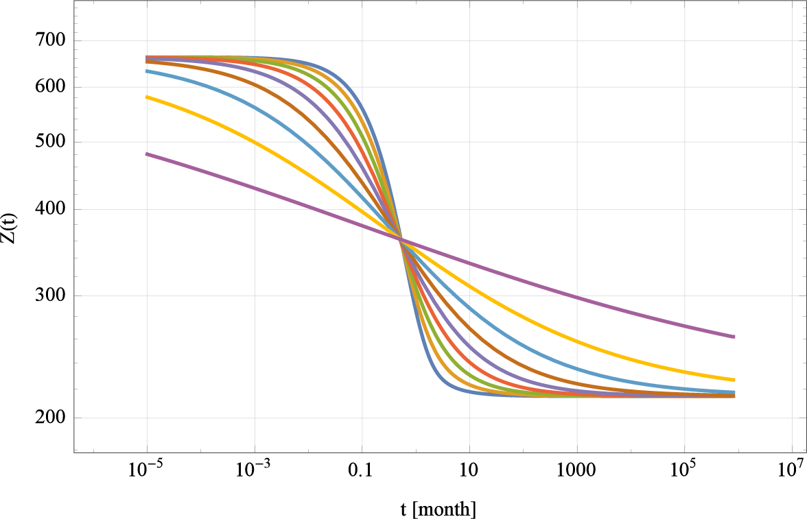
4.2. Extended Fractional Relaxation

In a paper examining primarily protein dynamics Glöckle and Nonnenmacher [44] derived a fractional relaxation equation possessing an analytic solution. It is well known today that for the generalization of a relaxation process which shows an exponential decay using the fractional counterpart is delivering as solution the generalization of the exponential function, a Mittag-Leffler function. In the same paper the two authors conjectured that the relaxation equation can be generalized to a driven fractional equation. At the time when the paper was written there was no method available to deal either analytically nor numerically with such kind of equation. In the next few lines we will show how such kind of driven fractional differential equation can be solved by Sinc methods using instead of a Rieman-Liouvill operator a Caputo fractional derivative.
The fractional differential equation which was solved by Glöckle and Nonnenmacher is given by
τ 0 β ϕ ( t ) + D 0 , t β ϕ ( t ) ϕ 0 t β Γ ( 1 β ) = 0 ,
which is equivalent to the fractional integral equation
τ 0 β D 0 , t β ϕ ( t ) + ϕ ( t ) ϕ 0 = 0 ,
Equation (84) allows the general analytic solution
ϕ ( t ) = ϕ 0 E β ( ( t / τ 0 ) β )
where Eβ(t) is the Mittag-Leffler function. Selecting the initial value and the relaxation constant as ϕ0 = 1 and τ0 = 1/10, we can straight forward approximate the solution by using the function RiemannLiouvilleFIE[] delivering for N = 32 Sinc points an accurate representation of the solution
solRLI = RiemannLiouvilleFIE [ 1 , ϕ , { t , 0 , 10 } , 1 / 2 , ( 10 ) 1 / 2 , 32 , 1 , 0 ] ;
The approximation and the local error of the approximation is shown in Figure 2. The local error (right panel) in Figure 2 is below an acceptable value of 10−4. If the number of Sinc points is increased this error decays exponentially.
Glöckle’s representation of the fractional differential equation includes the right hand side of the solution which is the sum over initial conditions.
τ 0 β ϕ ( t ) + D 0 , t β ϕ ( t ) ϕ 0 t β Γ ( 1 β ) = 0.
The term ϕ0 tβ/Γ(1 − β) is generated in the implemented solution; i.e., related to the initial value and thus not part of the Cauchy problem. Knowing this fact we are able to generate the approximation in two different ways using a function based on non-linear Caputo fractional differential equations. The first approach uses the linear term τ 0 β ϕ ( t ) as argument and treats the exogenous term separately.
solCC = CaputoNFD [ τ 0 β ϕ [ t ] / . { τ 0 1 / 10 , ϕ 0 1 , β 1 / 2 } , 0 , { 1 } , ϕ , { t , 0 , 10 } , 1 / 2 , 1 , 64 , 1 , 0 ] ;
The second approach uses the exogenous term as part of the equation. If we use the part of the initial values we can suppress the initial value and use the given representation as
sol = CaputoNFD [ τ 0 β ϕ [ t ] ϕ 0 ( t ) β Gamma [ 1 β ] / . { τ 0 1 / 10 , ϕ 0 1 , β 1 / 2 } , 0 , { 0 } , ϕ , { t , 0 , 10 } , 1 / 2 , 1 , 64 , 1 , 0 ] ;
The results of both approximations are shown in Figure 3. The top panel shows the two approximation approaches in addition to the exact solution. The bottom panel represents the local errors of the two different approximations. It becomes obvious that the second approximation is by 4 decades more accurate than the first approach. However, in both approximations the error is sufficient for an accurate representation of the exact result.
In Figure 4 we display approximations of the solution with varying β and fixed relaxation time τ0 and initial condition ϕ0. The approximation is performed by a Caputo fractional operator.
The generalization Glöckle and Nonnenmacher suggested is a fractional differential equation of the form
τ 0 β ϕ ( t ) + D 0 , t β ϕ ( t ) ϕ 0 t β Γ ( 1 β ) = χ 0 E ( t )
where E(t) is a harmonic function. Let us assume that E(t) = sin(πt) representing for example an external electric field applied to the relaxation process. The solution for such kind of equation is again generated by using the Caputo representation of the fractional derivative. An example for the selection of the amplitude χ0 = 1/10 is shown in Figure 5. The graphs shown in Figure 5 are the driven solution (solid line) and as a reference the solution of Equation (88) with χ0 = 0 using the same relaxation parameters. It is obvious that the driven solution follows the solution of the relaxation equation. The oscillations around the relaxation solution decay for larger times t. Note Figure 5 uses a logarithmic scale for ϕ(t).
Another way to generalize the relaxation equation is to include a nonlinearity into the equation. One interesting nonlinearity is a periodic function like in a mathematical pendulum. The equation without exogenous term may be written as
τ 0 β ϕ ( t ) + τ 0 β ϕ 1 sin ( ϕ ( t ) ) + D 0 , t β ϕ ( t ) ϕ 0 t β Γ ( 1 β ) = 0
Figure 6 shows the approximation of Equation (89) in connection with the original linear model Equation (84). The two curves in Figure 6 represent the original linear model Equation (84) (far right curve) and the non-linear model Equation (89) (far left curve), respectively. It is obvious that the difference between the two models is a shift along the t-axis possessing the same asymptotic scaling behavior.
This example demonstrates that fractional differential equations can be solved effectively with high accuracy if we use Sinc approximations. The variation of a model by extending it with exogenous or non-linear terms is in fact no problem for the used approximation method. In addition the error of the calculations decays exponential allowing a high precision representation of the approximation.

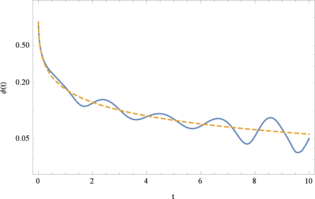
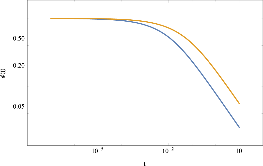
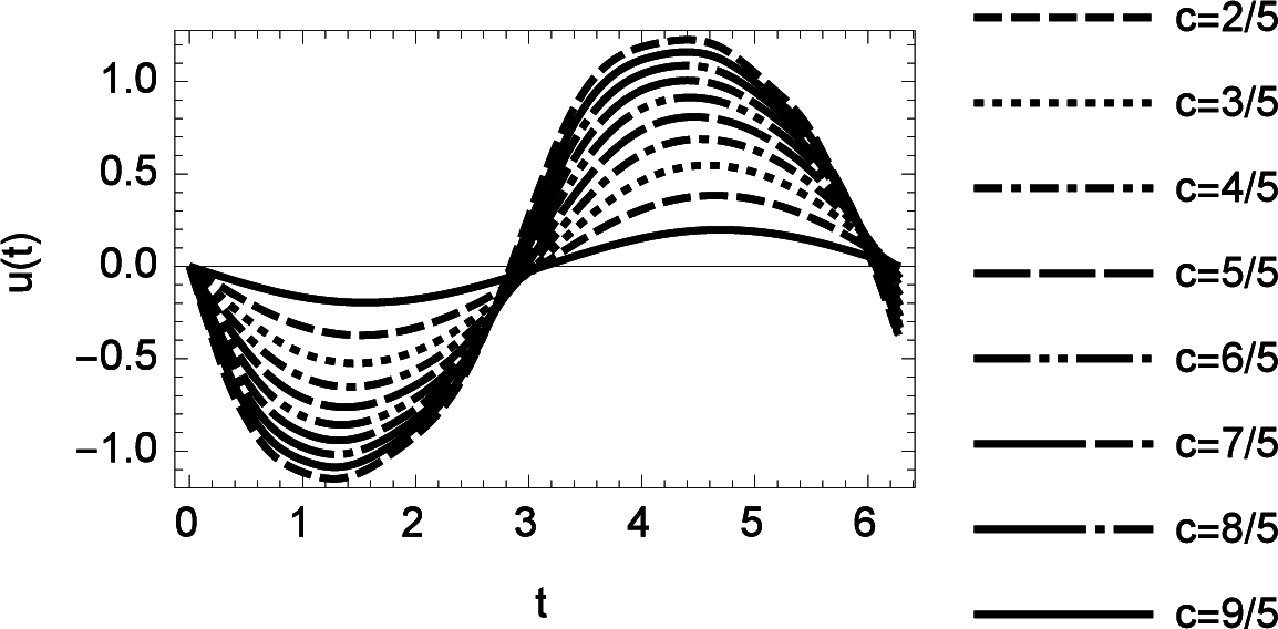
4.3. Fractal Filters

Modern design of electronic filters, such as low-pass, high-pass, and bandpass filters includes the construction of a rational function which satisfies the desired specifications for cutoff frequencies, pass-band gain, transition bandwidth, and stop-band attenuation. Recently these rational approximations were extended to fractal filters improving the design methodology in some direction. Following Podlubny [35] a fractional-order control system can be described by a fractional differential equation of the form:
a n D α n u ( t ) + a n 1 D α n 1 u ( t ) + + a 0 D α 0 u ( t ) = b m D β m u ( t ) + b m 1 D β m 1 u ( t ) + + b 0 D β 0 u ( t )
or by an equivalent continuous transfer function
G ( s ) = b m s β m + b m 1 s β m 1 + + b 0 s β 0 a n s α n + a n 1 s α n 1 + + a 0 s α 0 .
The use of the continuous transfer function is nowadays the standard approach to design filters. The transfer function Equation (91) uses however fractional exponents αi and βj to represent the fractional orders of the differential equations. One idea originally introduced by Roy is that the irrational transfer function G(s) can be replaced by a rational approximation G ˜ ( s ) [48]. Such kind of rational approximation can be performed by a Sinc point based Thiele algorithm [31]. Thiele’s algorithm basically converts a rational expression to a continued fraction representation which is related to a rational expression possessing exponents of natural numbers. Such kind of approximation will change of course the representation of the rational character of the transfer function but allows us to use a fraction with integer orders if we need to invert the Laplace transformation to the original domain. The advantage here is that for rational functions with integer powers there exists a well known method by Heaviside to invert a Laplace transform.
To demonstrate the procedure let us consider a simple fractional relaxation equation. The equation for a fractional relaxation process is given by
D q u ( t ) = τ q u ( t ) + u 0 t q Γ ( 1 q )
where 0 < q ≤ 1 is a positive number and u0 is the initial condition. The Laplace transform of the above equation delivers the algebraic equation
s q L t s u ( t ) = u 0 s q 1 τ q L t s u ( t )
the Laplace transform of u is denoted by L t s u ( t ). The solution of this equation in Laplace space follows by solving the above equation with respect to the Laplace representation of u:
L t s u ( t ) = u 0 s q 1 s q + τ q = G ( s ) .
Inverting this transfer function using inverse Laplace transforms and Mellin transforms [47] will deliver the exact solution
u ( t ) = u 0 E q ( ( t / τ ) q ) .
The derived function G(s) using a Laplace transform from is in terms of the more general systems theory the transfer function of the system with q ∈ ℝ. The definition of G allows us to perform the steps needed to approximate the irrational fraction by a rational one. First let us define G by
G ( s _ , u 0 _ , τ _ , q _ ) : = u 0 s q 1 s q + τ q
The number of Sinc points used in the calculation are
n = 17 ;
which also defines the step length for the inverse conformal map
h = π n ;
The Sinc points are generated next
SincPoints = N [ Table [ ψ ( h , k , 0 , ) , { k , n , n } ] ]
and used to map them to the basis points { ( s i , G ( s i ) ) } i = n n which are used in Thiele’s algorithm to generate the rational approximation. The parameters {u0, τ, q} used in the transfer function are given for this example by
parameters = { u 0 1 , τ 1 2 , q 2 3 } { u 0 1 , τ 1 2 , q 2 3 }
The data points of the transfer function G are then generated by the mapping
sincData = N [ ( { # 1 , G ( # 1 , u 0 , τ , q ) } & ) / @ sincPoints ] / . parameters
This set of data points is used in the Thiele continued fraction generation delivering the following expression
cf 2 = thieleContinuedFraction [ sincData , 2 n 2 ] / . x s
Mathematics 03 00444f18
Mathematics 03 00444f19
A rewriting of this continued fraction to a rational function is performed next. In addition we remove small quantities from this expression so that finally the rational expression follows
cf 2 = Simplify [ cf 2 ] / / Chop
Mathematics 03 00444f20
The result is an approximation of the transfer function G ( s ) G ˜ ( s ) = p m ( s ) / q n ( s ) where pm and qn are polynomials of order m and n satisfying mn, and m, n ∈ ℕ which is a prerequisite of Heaviside’s theorem. The approximated fraction G ˜ ( s ) and the original expression for the transfer function G(s) is shown in Figure 7. The left panel shows the original irrational fractional transfer function G(s) and its approximation using Thiele’s algorithm. It is obvious that between the original function and its approximation there is no visible difference. However, the local error between the exact and approximated function is shown in the right panel of Figure 7. We observe in this Figure that the error first is a small quantity and that for larger values of s the local error decays more than 4 decades.
If the approximation of the transfer function is known as a symbolic rational expression it becomes straight forward using Heaviside’s expansion theorem for inverse Laplace transforms to find the symbolic solution for the fractional relaxation equation. Heaviside’s theorem tells us that the fractional approximation can be represented in terms of exponential functions. The application of the inverse Laplace transform to the approximation of the transfer function G ˜ ( s ) delivers
u = Expand [ L s 1 [ cf 2 ] ( t ) ]
Mathematics 03 00444f21
which in fact represents the solution u(t) as an approximation in terms of exponential functions. This solution represents a continuous function which is shown in Figure 8.
The results shown in Figure 8 make it obvious that an approximation of the solution of a fractional initial value problem is a direct method and delivers an accurate result with a minimal amount of calculation steps. In fact the steps needed are reduced to the collocation of the transfer function which is approximated by Thiele’s algorithm as a continued fraction. This continued fraction is converted to a rational expression which is used in a Laplace inversion to get the solution. Such kind of inversion is always possible if the conditions for Heaviside’s expansion theorem are satisfied. Thus any rational fraction of polynomials can be represented by a finite sum of exponential functions if the inverse Laplace transform is applied to this rational fraction in Laplace space.
In another experiment we examine the convergence of the solution u(t) in case if the number of approximation points n are increased. Since there is only an estimation formula for Thiele’s algorithm which tells us that the error of approximation decays exponentially [31], we have to examine the error propagation after we have applied the inverse Laplace transform to the rational fraction G ˜ ( s ). However, since the inverse Laplace transform is carried out analytically we can assume that the error will not increase in this analytic step. In fact the numerical experiments show that the error decays exponentially after the application of the inverse Laplace transform. The decline of the global error based on the maximum norm follows a relation given by ϵ(n) = a exp (−bnc) where a, b, and c are independent of n. The decay of ϵ(n) is shown in Figure 9 for a specific example. The dots in this figure represent the maximum norm of the error while the solid line represents a least square fit to these data using the predicted error formula.
A model using exponential approximations was discussed in a quite different, biological, field examining the binding of oxygen in blood cells. Glöckle and Nonnenmacher used a transfer function in connection with protein dynamics in blood cells [44]. The claim of the paper was that protein dynamics described in a standard approach as a superposition of many relaxation processes by a series of exponential functions as
u ( t ) = n w n exp ( ( t / τ n ) )
can be unified to a fractional relaxation equation of type Equation (92) where the weights wn and relaxation times τn satisfy a certain scaling relation [44]. In view of the method applied here such kind of scaling relation is naturally inherited by the Haeviside expansion theorem. According to Heaviside’s theorem the inverse relaxation times are the roots of the denominator polynomial of G ˜ ( s ) and the weights are calculated from w n = p μ ( 1 / τ n ) / q ν ( 1 / τ n ). To demonstrate that such scaling behavior naturally is included in Heaviside’s theorem, we analyzed an approximation with 40 exponential terms. Our observation is that there exist two scaling regimes with the same scaling exponent but with opposite sign. The two regimes are glued together at τ ≈ 1. The slopes of the two scaling regimes are ω = ±0.67512 for the parameters selected above. We note that q = 2/3 for this calculation. The scaling behavior is shown in Figure 10 where the weights wn as a function of the inverse of the relaxation times τn are shown in a double logarithmic plot. This log − log plot directly shows the scaling regions indicated by straight lines. The slopes determined by a least square fit for each of these regions was ω as given above. The scaling is present for at least 6 decades for both regions.
In fact the scaling relation in [44] was based on experimental data for rebinding of CO to Mb after photo dissociation [45]. These experimental data were represented by a sum of exponential functions as stated in Equation (96). However, it is quite interesting that Nonnenmacher and Nonnenmacher [46] derived scaling relations which are close to our estimations but based on a quite different approach using Markov chains.
To exemplify the scaling behavior for our calculations we also performed calculations with different fractional order q. It turned out that the slope of the scaling exponent determined in a least square fit is approximately representing the fractional order q. These relations are shown in Figure 11. This figure summarizes the calculations for different fractional orders q in a single plot. It becomes obvious that the transition from positive to negative scaling slopes occurs around τ ≈ 1. While for smaller q’s there is a smooth transition for larger q values this change of slope occurs more rapidly.
The conclusion of this example is that a rational approximation based on Thiele’s algorithm is very effective if we have to solve initial value problems approximated or represented by rational transfer functions. For such cases the inverse Laplace transform is delivering the solution if the prerequisites of the Heaviside expansion theorem are satisfied. Knowing that the final solution of a fractional relaxation equation can be represented as a sum of exponential functions it becomes consistent with experimental findings that a rational approximation of a fractal transfer function is related to the fractal behavior of the physical system. In other words whenever a physical system allows a sum of exponential functions there is a chance that the system shows fractal behavior.

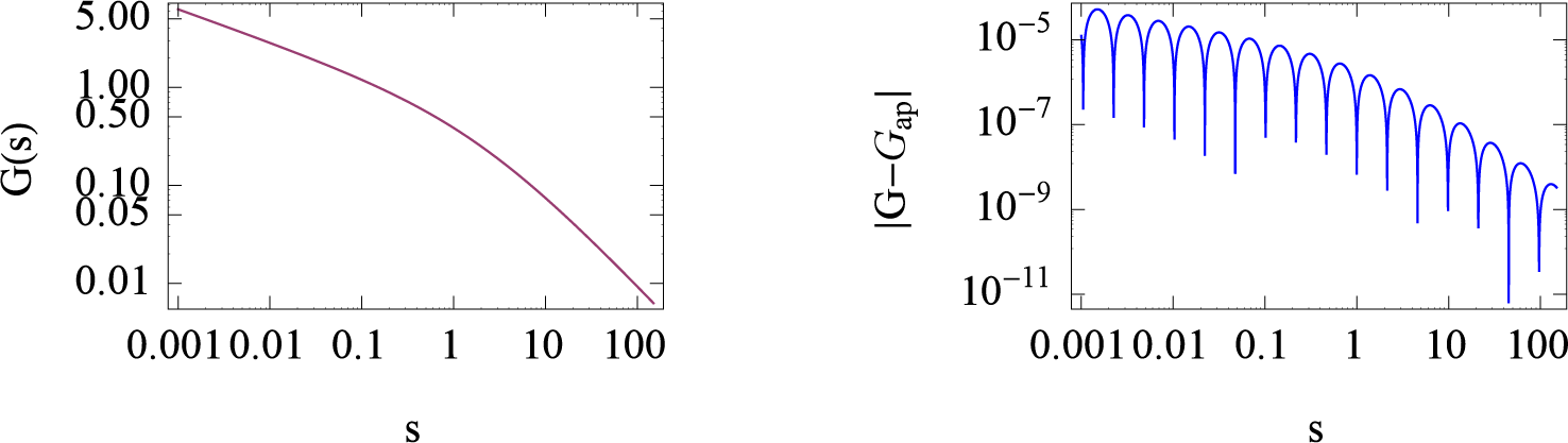
4.4. Inverse Laplace Transform

Knowing the facts about Sinc methods of convolution representations of integral equations and the property of linear systems allowing a fractional algebraic representation by a transfer function, we can take another route to find an approximation of the solution by using the inverse Laplace transform. The inverse Laplace transform is a spin off of the definition of the Laplace transform in Equation (24). The inverse transform of Laplace can be generated the following way.
Let the “Laplace transform” F be defined as in Equation (24). If J denotes the indefinite integral operator defined on (0, a) ⊂ (0, c) ⊂ (0, ∞), then [29,31]
f = ( J ) 1 F ( J ) 1 ,
where “1” denotes the function that is identically 1 on (0, a). Hence, with J m w T A + V, with A m + = X + Σ ( X + ) 1, Σ = diag (s−M, …, sN), we can proceed as follows to approximate f:
  • Assume that the spectrum; i.e., the matrix X+ and vector s = (s−M, …, sN)T have already been stored for some interval (α, β), corresponding to matrix A m +, make the replacement sα/(βα)s, and compute the column vector v = (vM, …vN)T = (X+)−1 1, where 1 is a vector of M + N + 1 ones;
  • Compute
    g = ( F ( s M ) / s M , , F ( s N ) / s N ) ,
    x = g * v with * a Hadamard product ,
    f = ( f M , , f N ) T = X + z .
  • All operations of this evaluation take a trivial amount of time, except for the last matrix vector equation. However, the size of these matrices is nearly always much smaller than the size of the DFT matrices for solving similar problems via FFT.
Then we have the approximation f (xj) ≈ fj, which we can combine, if necessary, with our interpolation Formula (11) to get a continuous approximation of f on (0, a).
An example we already discussed above is related to the relaxation equation. It’s transfer function is defined in general as
G ( s _ , u 0 _ τ _ , q _ ) : = u 0 s q 1 s q + τ q
Specifying the related parameters
parameters = { u 0 1 , τ 1 2 , q 2 7 } ;
we get the specific representation of the transfer function for any q and relaxation time τ as follows
g 1 = G ( s , u 0 , τ , q ) / . parameters 1 ( s 2 / 7 + 2 2 / 7 ) s 5 / 7
The inverse Laplace transform of this transfer function delivers the time dependent relaxation function as shown in Figure 12.
sol 1 = stengerInverseLaplaceTransform [ g 1 , { s } , { t , 0 , 100 } , 1 , 0 , 32 ] ;
Now it becomes straight forward to determine the time domain behavior of a system if the transfer function G(s) is known. A practical example of such an application is the modeling of ultracapacitors [49]. Ultracapacitors or electrochemical double layer capacitors are handled as energy storage devices which may replace batteries due to their high capacity and long standing high energy density [50,51]. As a result, ultracapacitors are becoming more widely used in energy storage systems especially in mobility applications [5052]. Such an ultracapacitor can be modeled as a ladder of resistors and capacitors building up an RC transmission line; for details see [49]. The impedance transfer function of such a model has the structure
t e x t Z s = 664 ( s 3 + 2 3 ) s ( s 3 + 2.06 ) ;
The numeric terms are due to the scaling given in time steps of months. The time dependent impedance of such a model now directly follows via the inverse Laplace transform for a large range approximation by
sol 3 = stengerInverseLaplaceTransform [ Z s , { s } , { t , 0 , 10 6 } , 1 , 0 , 128 ] ;
It is obvious from the long term and short term behavior of the time dependent impedance that two plateaus exist (see Figure 13). One for the short time behavior which lasts about 10−4 months which corresponds approximately to 45 min. The second plateau stabilizes on a level of approximately 220 after 103 month corresponding to approx. 83 years. The drop from a level of about 640 to 300 lasts about 8 month. With such a characteristic the device is a highly promising energy storage device to replace the electrochemical based batteries.
It becomes also straight forward to examine the impedance model for different fractional orders q if we generalize the model in [49] to the following relation
zS 4 = 448 2.06 s q + s + 215 s ;
The inverse Laplace transform for a sequence of fractional exponents is generated in the following line based on the sequence q { i 10 } i = 1 9 in a parallel calculation for each of the exponents q
sol 4 = ParallelTable [ { q , stengerInverseLaplaceTransform [ zS 4 , { s } , { t , 0 , 10 6 } , 1 , 0 , 128 ] } , { q , 1 / 10 , 9 / 10 , 1 / 10 } ] ;
The results of these calculations are shown in Figure 14. It becomes apparent that the drop in the impedance is more rapidly for smaller fractal exponents than for lager ones 0 < q < 1 which may be a design indication.
This example demonstrates that Sinc methods are effective especially for practical engineering applications. The inverse Laplace transform of a linear fractional differential/integral equation is accessible with a minimum amount of calculation steps and a high accuracy.

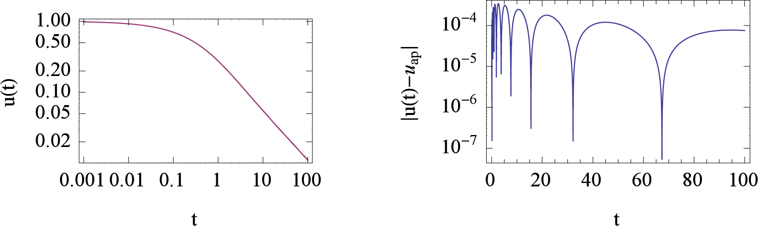
4.5. Levinson’s Integral Equation

Finally we discuss a model which originally was not formulated as a fractional model but in retrospect can be interpreted as such. Levinson in 1960 [40] based on a paper by Lin on the hydrodynamics of liquid Helium [41] derived in a paper about super-fluidity the following non-linear Volterra equation of second kind
u ( t ) + 1 π 0 t ( t τ ) 1 / 2 u ( τ ) 3 d τ = c sin ( t ) .
Applying to Equation (101) the notation of fractional calculus we realize that this equation is equivalent to a non-linear fractional differential equation of the following form
D 0 , t 1 / 2 u ( t ) + u ( t ) 3 = c π t E 2 , 2 / 3 ( t 2 )
using the initial condition u(0) = 0 and where Eα,β(t) denotes the generalized Mittag-Leffler function. Levinson proved in his paper that a solution of the nonlinerar integral equation exists and may be derived by successive iterations as an approximation. We take the position here that the existence of the solution is guaranteed by the proof of Levinson and approximate such kind of solution by applying non-iterative Sinc methods to Equation (102). The steps of the calculation are implemented in a function RiemannLiouvilleNonlinearFIE[] which sets us into position to directly solve the equation if we specify the non-linearity of the integral and the exogenous function g(t) = −c sin(t). The following line performs the calculation with a fractional order α = 1/2, with λ = 1 / π, and N = 64 Sinc points
solution = RiemannLiouvilleNonlinearFIE [ [ t ] 3 , 6 / 5 Sin [ t ] , u , { t , 0 , 2 π } , 1 / 2 , 1 π , 64 , 1 , 0 ] ;
The solution u(t), u(t) + (6/5) sin(t), and (6/5) sin(t) are shown on the interval t ∈ [0, 2π] in the following Figure 15. In this Figure we compare the solution u(t) with the exogenous driving function and the addition of u and the driver function. It is apparent that the solution of the non-linear integral equation is not related any more to the exogenous function as the linear theory delivers. The structure of the solution is distorted but shows an oscillating structure nearly with the same period as the exogenous function.
The amplitude of the solution can be controlled by the amplitude c of the exogenous function. Different amplitudes are shown in Figure 16. The choice of c also has some small influence on the period of the oscillation.
If we understand Levinson’s integral equation as a fractional integral equation, we can also ask for a generalization with a fractional exponent μ { 1 / k } k = 2 6 as
D 0 , t 1 / k u ( t ) + u ( τ ) 3 = c π t E 2 , 2 / 3 ( t 2 ) with , k = 2 , 3 ,
The results of such variation of is shown in Figure 17.

5. Conclusions

The different models examined here demonstrate that Sinc methods are well equipped to deal with fractional differential or integral equations. The Sinc approach to approximate convolution integrals is one of the keys to deal with linear and non-linear fractional equations delivering with a minimal amount of calculations a highly accurate result. If the equations are linear the approach of the transfer function becomes effective in connection with Thiele’s algorithm and with a direct inversion of the Laplace transform. Both methods based on transfer functions are using Sinc points as discrete points which are a nearly optimal choice of the discrete mesh if the Lebesgue measure is used. The discussed models also demonstrate that the misnomer “fractal” equation is only on spot if the solution shows an asymptotic scaling law. From the variety of solutions generated with these few examples it seems to be more precise to call the “fractal” equations fractional equations which reflects more the diversity of solutions of such equations. Since all the fractional equations are singular integral or differential equations the Sinc method proves once more that it is self-sufficient of the singular behavior.

Acknowledgments

We acknowledge the support by N. Südland in symbolic computer algebra calculations with Fractional Calculus.
MSC classifications: 65D05, 65D30, 44A35, 81-04

Author Contributions

Gerd Baumann and Frank Stenger performed the calculations and computations in close cooperation. The manuscript was written by both authors in an effective teamwork.

Conflicts of Interest

The authors declare no conflict of interest.

References

  1. Oldham, K.B.; Spanier, J. The Fractional Calculus; Academic Press: New York, NY, USA, 1974. [Google Scholar]
  2. Abel, N.H. Auflösung einer mechanischen Aufgabe. J. Reine Angew. Math. 1826, 1, 153–157. [Google Scholar]
  3. Kilbas, A.A.; Srivastava, H.M.; Trujillo, J.J. Theory and Applications of Fractional Differential Equations; Elsevier: Amsterdam, The Netherlands, 2006. [Google Scholar]
  4. Freed, A.D.; Diethelm, D.K. Fractional calculus in biomechanics: A 3D viscoelastic model using regularized fractional derivative kernels with application to the human calcaneal fat pad. Biomech. Mod. Mech. 2006, 5, 203–215. [Google Scholar]
  5. Schmidt, A.; Gaul, L. FE Implementation of Viscoelastic Constitutive Stress-Strain Relations Involving Fractional Time Derivatives. Const. Model. Rubber 2001, 2, 79–92. [Google Scholar]
  6. Lubich, Ch. Convolution Quadrature and Discretized Operational Calculus I. Numer. Math. 1988, 52, 129–145. [Google Scholar]
  7. Lubich, Ch. Convolution Quadrature and Discretized Operational Calculus II. Numer. Math. 1988, 52, 413–425. [Google Scholar]
  8. Agrawal, O.P.; Kumar, P. Comparison of five numerical schemes for fractional differential equations. In Advances in Fractional Calculus: Theoretical Developments and Applications in Physics and Engineering; Sabatier, J., Agrawal, O.P., Machado, J.A.T., Eds.; Springer: Dordrecht, The Netherlands, 2007; pp. 43–60. [Google Scholar]
  9. Lubich, Ch. Runge-Kutta theory for Volterra and Abel integral equations of the second kind. Math. Comput. 1983, 41, 87–102. [Google Scholar]
  10. Yuan, L.; Agrawal, O.P. A Numerical Scheme for Dynamic Systems Containing Fractional Derivatives. J. Vib. Acoust. 2002, 124, 321–324. [Google Scholar]
  11. Momania, S.; Odibatb, Z. Homotopy perturbation method for non-linear partial differential equations of fractional order. Phys. Lett. A 2007, 365, 345–350. [Google Scholar]
  12. Diethelm, K.; Ford, N.J.; Freed, A.D.; Luchko, Y. Algorithms for the fractional calculus: A selection of numerical methods. Comput. Methods Appl. Mech. Eng. 2005, 194, 743–773. [Google Scholar]
  13. Diethelm, K. The Analysis of Fractional Differential Equations: An Application-Oriented Exposition Using Differential Operators of Caputo Type; Springer: Heidelberg, Germany, 2010. [Google Scholar]
  14. Sabatier, J.; Agrawal, O.P.; Machado, J.A.T. Advances in Fractional Calculus: Theoretical Developments and Applications in Physics and Engineering; Springer: Dordrecht, The Netherlands, 2007. [Google Scholar]
  15. McNamee, J.; Stenger, F.; Whitney, E.L. Whittaker’s Cardinal Function in Retrospect. Math. Comput. 1971, 23, 141–154. [Google Scholar]
  16. Stenger, F. Collocating convolutions. Math. Comput. 1995, 64, 211–235. [Google Scholar]
  17. Adomian, G. Solving Frontier Problems of Physics: The Decomposition Method; Kluwer Academic Publisher: Dordrecht, The Netherlands, 1994. [Google Scholar]
  18. Edwards, J.T.; Roberts, J.A.; Ford, N.J. A Comparison of Adomiannal Differential Equations: An Application-Oriented Exposition Using Differential Operators of Caputo Type; Numerical Analysis Report; Manchester Centre for Computational Mathematics, University of Manchester: Manchester, UK, 1997; Volume 309, pp. 1–18. [Google Scholar]
  19. Répaci, A. Nonlinear dynamical systems: On the accuracy of Adomian’s decomposition method. Appl. Math. Lett. 1990, 3, 35–39. [Google Scholar]
  20. He, J.H. Approximate solution of non linear differential equations with convolution product nonlinearities. Comput. Meth. Appl. Mech. Eng. 1998, 167, 69–73. [Google Scholar]
  21. He, J.H. Variational iteration method—Some recent results and new interpretations. J. Comput. Appl. Math. 2007, 207, 3–17. [Google Scholar]
  22. Liao, S. Beyond Perturbation: Introduction to the Homotopy Analysis Method; Chapman & Hall/CRC Press: Boca Raton, FL, USA, 2004. [Google Scholar]
  23. Odibata, Z.; Momanib, S.; Erturkc, V.S. Generalized differential transform method: Application to differential equations of fractional order. Appl. Math. Comput. 2008, 197, 467–477. [Google Scholar]
  24. Tataria, M.; Dehghan, M. On the convergence of He’s variational iteration method. J. Comput. Appl. Math. 2007, 207, 121–128. [Google Scholar]
  25. Liang, S.; Jeffreya, D.J. Comparison of homotopy analysis method and homotopy perturbation method through an evolution equation. Commun. Nonlinear Sci. Numer. Simul. 2009, 14, 4057–4064. [Google Scholar]
  26. Stenger, F. Summary of Sinc numerical methods. J. Comput. Appl. Math. 2000, 121, 379–420. [Google Scholar]
  27. Gavrilyuk, I.P.; Hackbusch, W.; Khoromskij, B.N. Data-Sparse Approximation to a Class of Operator-Valued Functions. Math. Comput. 2005, 74, 681–708. [Google Scholar]
  28. Khoromskij, B.N. Fast and Accurate Tensor Approximation of a Multivariate Convolution with Linear Scaling in Dimension. J. Comput. Appl. Math. 2010, 234, 3122–3139. [Google Scholar]
  29. Stenger, F. Handbook of Sinc Numerical Methods; CRC Press: Boca Raton, FL, USA, 2011. [Google Scholar]
  30. Kowalski, M.A.; Sikorski, K.A.; Stenger, F. Selected Topics in Approximation and Computation; Oxford University Press: New York, NY, USA, 1995. [Google Scholar]
  31. Stenger, F. Numerical Methods Based on Sinc and Analytic Functions; Springer: New York, NY, USA, 1993. [Google Scholar]
  32. Burchard, H.G.; Höllig, K. N-Width and Entropy of Hp-Classes in Lq(−1, 1). SIAM J. Math. Anal. 1985, 16, 405–421. [Google Scholar]
  33. Stenger, F.; El-Sharkawy, H.; Baumann, G. The Lebesgue Constant for Sinc Approximations. In New Perspectives on Approximation and Sampling Theory; Zayed, A.I., Schmeisser, G., Eds.; Springer International Publishing: New York, NY, USA, 2014; pp. 319–335. [Google Scholar]
  34. Capuro, M.; Mainardi, F. A new dissipation model based on memory mechanism. Pure Appl. Geophys. 1971, 91, 134–147. [Google Scholar]
  35. Podlubny, I. Fractional Differential Equations: An Introduction to Fractional Derivatives, Fractional Differential Equations, to Methods of Their Solution and Some of Their Applications; Academic Press: San Diego, CA, USA, 1999. [Google Scholar]
  36. Baumann, G.; Stenger, F. Fractional Calculus and Sinc Methods. Fract. Calc. Appl. Anal. 2011, 14, 1–55. [Google Scholar]
  37. Han, L.; Xu, J. Proof of Stenger’s conjecture on matrix of Sinc methods. J. Comput. Appl. Math. 2014, 255, 805–811. [Google Scholar]
  38. Miller, K.S.; Ross, B. An Introduction to the Fractional Calculus and Fractional Differential Equations; Wiley: New York, NY, USA, 1993. [Google Scholar]
  39. Daftardar-Gejji, V.; Jafari, H. Analysis of a system of nonautonomous fractional differential equations involving Caputo derivatives. J. Math. Anal. Appl. 2007, 328, 1026–1033. [Google Scholar]
  40. Levinson, N. A nonlinear equation arising in the theory of superfluidity. J. Math. Anal. Appl. 1960, 1, 1–11. [Google Scholar]
  41. Lin, C.C. Hydrodynamics of Liquid Helium II. Phys. Rev. Lett. 1959, 2, 245–246. [Google Scholar]
  42. Dietheln, K.; Ford, N.J. Numerical solution of the Bagley Torvik equation. BIT Numer. Math. 2002, 42, 490–507. [Google Scholar]
  43. Diethelm, K. Efficient solution of multi-term fractional differential equations using P(EC)mE methods. Computing 2003, 71, 305–319. [Google Scholar]
  44. Glöckle, W.G.; Nonnenmacher, T.F. A fractional calculus approach to self-similar protein dynamics. Biophys. J. 1995, 68, 46–53. [Google Scholar]
  45. Austin, R.H.; Beeson, K.W.; Eisenstein, L.; Frauenfelder, H.; Gunsalus, I.C. Dynamics of ligand binding to myoglobin. Biochemistry 1975, 14, 5355–5373. [Google Scholar]
  46. Nonnenmacher, T.F.; Nonnenmacher, D.J.F. A Fractal Scaling Law for Protein Gating Kinetics. Phys. Lett. A 1989, 140, 323–326. [Google Scholar]
  47. Baumann, G. Mathematica for Theoretical Physics; Springer: New York, NY, USA, 2013; Volume I and II. [Google Scholar]
  48. Roy, S.D. On the Realization of a Constant-Argument Immittance or Fractional Operator. IEEE Trans. Circuit Theory 1967, 14, 264–274. [Google Scholar]
  49. Wang, Y.; Hartley, T.T.; Lorenzo, C.F.; Adams, J.L.; Carletta, J.E.; Veillette, R.J. Modeling Ultracapacitors as Fractional-Order Systems. In New Trends in Nanotechnology and Fractional Calculus Applications; Baleanu, D., Güvenç, Z.B., Machado, J.A.T., Eds.; Springer: Dordrecht, The Netherlands, 2010; pp. 257–262. [Google Scholar]
  50. Belhachemi, F.; Rael, S.; Davat, B. A physical based model of power electric doublelayer supercapacitors, Proceedings of the 2000 IEEE Industry Applications Conference, Rome, Italy, 8–12 October 2000; 5, pp. 3069–3076.
  51. Mellor, P.H.; Schofield, N.; Howe, D. Flywheel and supercapacitor peak power buffer technologies, Proceedings of the IEEE Seminar on Electric, Hybrid and Fuel Cell Vehicles, Durham, UK; 2000; 8, pp. 1–5.
  52. Schupbach, R.M.; Balda, J.C. The Role of ultracapacitors in an energy storage unit for vehicle power management, Proceedings of the 2003 IEEE 58th Vehicular Technology Conference, Orlando, FL, USA, 6–9 October 2003; 5, pp. 3236–3240.
Figure 1. Riemann-Liouville integral of order v = −1/3 of the function f(x) = eax where a = 1 (top panel). Shown are also the locations of the Sinc points along the solution. The bottom panel shows the local error for N = 32 Sinc points.
Mathematics 03 00444f1
Figure 2. Approximations of the fractional relaxation Equation (84) using the fractional order β = 1/2. The initial condition and the relaxation time τ0 was set to ϕ0 = 1 and τ0 = 1/10. The solid line represents the analytic solution E1(−10t). The Sinc approximation of the Riemann-Liouville representation used N = 32 Sinc points.
Mathematics 03 00444f2
Figure 3. Approximations of the fractional relaxation Equation (84) using the fractional order β = 1/2 in a Caputo fractional representation. The initial condition and the relaxation time τ0 was set to ϕ0 = 1 and τ0 = 1/10. The solid line represents the analytic solution E1(−10t). The Sinc approximation of the Caputo representation used N = 64 Sinc points.
Mathematics 03 00444f3
Figure 4. Approximations of the fractional relaxation Equation (84) using different fractional orders β. The initial condition and the relaxation time τ0 was set to ϕ0 = 1 and τ0 = 1/10. The solid line represents the analytic solution E1(−10t). The Sinc approximation of the Caputo representation used N = 64 Sinc points.
Mathematics 03 00444f4
Figure 5. Approximations of the driven fractional relaxation Equation (88) (solid line). The initial condition and the relaxation time τ0, the amplitude of the driving force χ0, and the fractional order was β set to ϕ0 = 0, τ0 = 1/10, χ0 = 1/10, and β = 1/2. The dased line represents the solution of the relaxation Equation (84) using the same parameters. The Sinc approximation of the Caputo representation used N = 64 Sinc points.
Mathematics 03 00444f5
Figure 6. Non-linear fractional relaxation equation (89) (upper line). The initial condition and the relaxation time τ0, and the fractional order β was set to ϕ0 = 1, τ0 = 1/10, ϕ1 = 25/20, and β = 1/2. The lower curve represents the solution of the relaxation equation (84) using the same parameters. The Sinc approximation of the Caputo representation used N = 64 Sinc points.
Mathematics 03 00444f6
Figure 7. Approximation of the transfer function G(s) for a fractional relaxation equation given by Equation (94). The left panel shows the exact transfer function G(s) with u0 = 1, τ = 1/2, and q = 2/3 in connection with the approximation using Thiele’s algorithm. The right panel shows the local error between the exact function and its approximation. The total number of point used in the approximation is m = 2n + 1 = 35.
Mathematics 03 00444f7
Figure 8. Solution of the fractional relaxation Equation (92) generated by the inverse Laplace transform of G ˜ ( s ). The left panel also includes the exact solution of the fractional relaxation equation given by u(t) = u0Eq (−(t/τ)q) where Eq(t) is the Mittag-Leffler function. The right panel shows the local error between the exact solution and the approximation. The number of approximation points used in the calculation was m = 2n + 1 = 35. The parameters to generate the plot are α = 1, τ = 1/2, q = 2/3.
Mathematics 03 00444f8
Figure 9. Maximum norm error ϵ(n) = |u(t) − uap| of the solution on the interval t ∈ [0, 10]. The error decay follows the relation ϵ = a exp (−bnc).
Mathematics 03 00444f9
Figure 10. Scaling regions of the weights wn as a function of 1/τn for a solution with 40 exponential functions and parameter values u0 = 1, τ = 1/2, q = 2/3, and n = 50.
Mathematics 03 00444f10
Figure 11. Scaling regions of the weights wn as a function of 1/τn’s for a solution with 40 exponentials and parameter values u0 = 1, τ = 1/2, q = {1/3, 1/2, 2/3, 3/4, 8/9}, and n = 51. The upper lines correspond to q = 1/3 while the lower line is assigned to q = 8/9.
Mathematics 03 00444f11
Figure 12. Solution of the fractional relaxation Equation (87) generated by the direct inverse Laplace transform of G(s). The left panel also includes the exact solution of the fractional relaxation equation given by u(t) = u0Eq (−(t/τ)q) where Eq(t) is the Mittag-Leffler function. The right panel shows the local error between the exact solution and the approximation. The number of approximation points used in the calculation was m = 2n + 1 = 65. The parameters to generate the plot are u0 = 1, τ = 1/2, q = 2/7.
Mathematics 03 00444f12
Figure 13. Time dependent impedance Z(t) derived from the inverse Laplace transform of the ultracapacitor.
Mathematics 03 00444f13
Figure 14. Time dependent impedance Z(t) derived from the inverse Laplace transform of the ultracapacitor with different fractal exponents q { i / 10 } i = 1 9. The steepest transition corresponds to q = 1/10.
Mathematics 03 00444f14
Figure 15. Solution of Levinson’s non-linear Volterra integral equation.
Mathematics 03 00444f15
Figure 16. Solution of Levinson’s non-linear Volterra integral equation for variations of c in the range of { c } c = 1 / 5 2 , 1 / 5.
Mathematics 03 00444f16
Figure 17. Solution of Levinsons non-linear Volterra integral equation for variations of μ= 1/k in the range of { 1 / k } k = 2 6.
Mathematics 03 00444f17

