On the Folded Normal Distribution

Abstract
:1. Introduction
2. The Folded Normal
2.1. Relations to Other Distributions
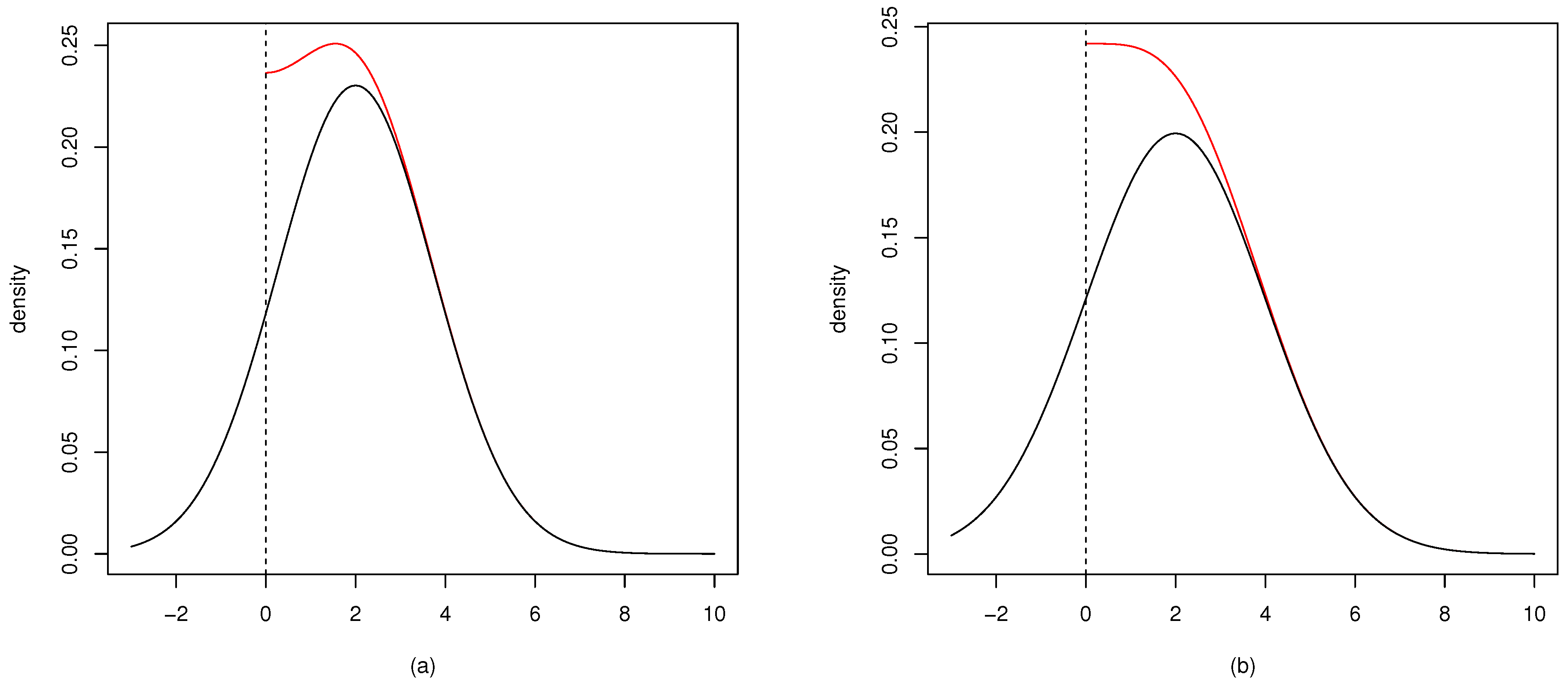
2.2. Mode of the Folded Normal Distribution
2.3. Characteristic Function and Other Related Functions of the Folded Normal Distribution
- The moment generating function of Equation (2) exists and is equal to:We can see that the characteristic generating function can be differentiated infinitely many times, since the first derivative contains the density of the normal distribution, and thus, it always contains some exponential terms. The folded normal distribution is not a stable distribution. That is, the distribution of the sum of its random variables do not form a folded normal distribution. We can see this from the characteristic (or the moment) generating function Equation (22) or Equation (23).
- The cumulant generating function is simply the logarithm of the moment generating function:
- The Laplace transformation can easily be derived from the moment generating function and is equal to:
- The Fourier transformation is:However, this is closely related to the characteristic function. We can see that . Thus, Equation (26) becomes:
- The mean residual life is given by:where . The above conditional expectation is given by:The denominator in Equation (30) is written as . The contents within the integral in the numerator of Equation (30) could be replaced by , as well, but we will not replace it. The calculation of the numerator is done in the same way as the calculation of the mean. Thus:Finally, Equation (30) can be written as:
3. Entropy and Kullback–Leibler Divergence
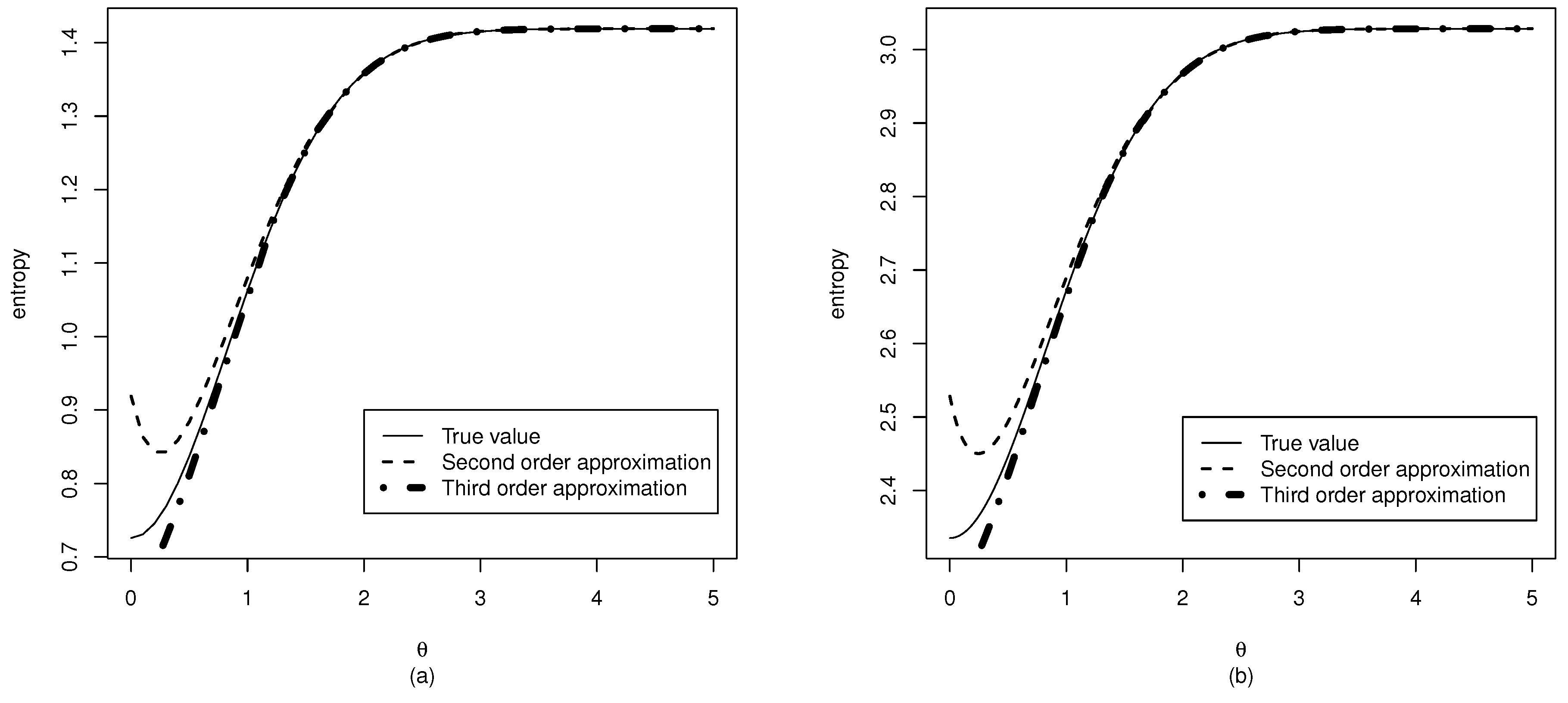
3.1. Entropy

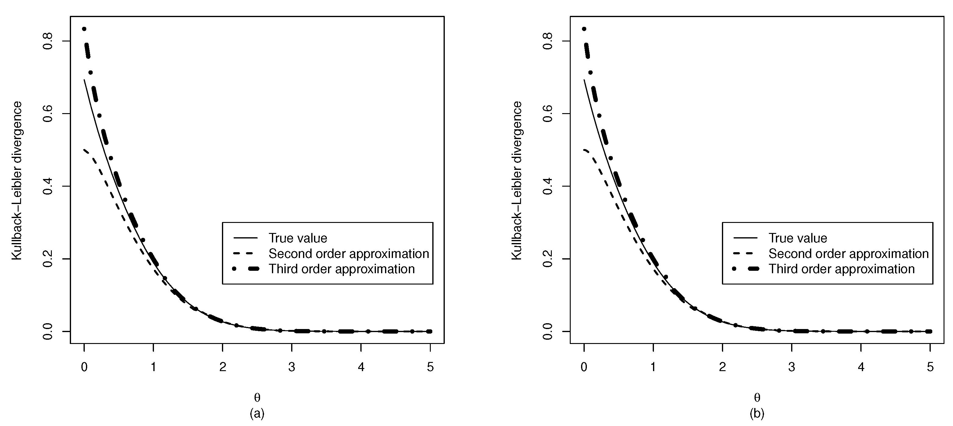
3.2. Kullback–Leibler Divergence from the Normal Distribution

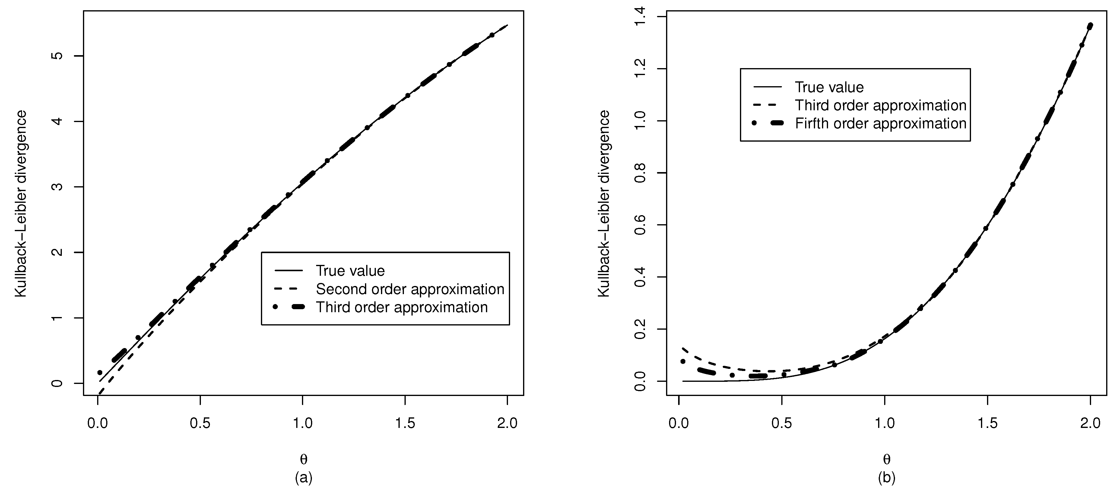
3.3. Kullback–Leibler Divergence from the Half Normal Distribution

4. Parameter Estimation
4.1. An Example with Simulated Data

4.2. Simulation Studies

| Values | of | θ | ||||||
|---|---|---|---|---|---|---|---|---|
| Sample size | 0.5 | 1 | 1.5 | 2 | 2.5 | 3 | 3.5 | 4 |
| 20 | 0.689 | 0.930 | 0.955 | 0.931 | 0.926 | 0.940 | 0.930 | 0.948 |
| 30 | 0.679 | 0.921 | 0.949 | 0.943 | 0.925 | 0.926 | 0.941 | 0.915 |
| 40 | 0.690 | 0.916 | 0.936 | 0.933 | 0.941 | 0.948 | 0.944 | 0.928 |
| 50 | 0.718 | 0.944 | 0.955 | 0.938 | 0.933 | 0.948 | 0.946 | 0.946 |
| 60 | 0.699 | 0.950 | 0.968 | 0.948 | 0.949 | 0.941 | 0.942 | 0.946 |
| 70 | 0.721 | 0.931 | 0.956 | 0.939 | 0.939 | 0.939 | 0.949 | 0.945 |
| 80 | 0.691 | 0.930 | 0.950 | 0.940 | 0.946 | 0.936 | 0.945 | 0.939 |
| 90 | 0.720 | 0.932 | 0.960 | 0.949 | 0.949 | 0.939 | 0.954 | 0.944 |
| 100 | 0.738 | 0.945 | 0.949 | 0.938 | 0.943 | 0.926 | 0.946 | 0.952 |
| Values | of | θ | ||||||
|---|---|---|---|---|---|---|---|---|
| Sample size | 0.5 | 1 | 1.5 | 2 | 2.5 | 3 | 3.5 | 4 |
| 20 | 0.890 | 0.925 | 0.939 | 0.921 | 0.918 | 0.940 | 0.929 | 0.942 |
| 30 | 0.894 | 0.931 | 0.933 | 0.943 | 0.926 | 0.922 | 0.942 | 0.910 |
| 40 | 0.910 | 0.925 | 0.927 | 0.933 | 0.941 | 0.947 | 0.946 | 0.928 |
| 50 | 0.914 | 0.943 | 0.942 | 0.934 | 0.934 | 0.945 | 0.946 | 0.943 |
| 60 | 0.904 | 0.949 | 0.953 | 0.950 | 0.941 | 0.938 | 0.943 | 0.944 |
| 70 | 0.893 | 0.934 | 0.943 | 0.936 | 0.937 | 0.938 | 0.949 | 0.939 |
| 80 | 0.918 | 0.940 | 0.939 | 0.939 | 0.944 | 0.935 | 0.946 | 0.938 |
| 90 | 0.920 | 0.934 | 0.952 | 0.948 | 0.946 | 0.939 | 0.951 | 0.947 |
| 100 | 0.918 | 0.940 | 0.936 | 0.932 | 0.946 | 0.925 | 0.945 | 0.949 |
| Values | of | θ | ||||||
|---|---|---|---|---|---|---|---|---|
| Sample size | 0.5 | 1 | 1.5 | 2 | 2.5 | 3 | 3.5 | 4 |
| 20 | 0.649 | 0.765 | 0.854 | 0.853 | 0.876 | 0.870 | 0.862 | 0.885 |
| 30 | 0.697 | 0.794 | 0.870 | 0.898 | 0.892 | 0.898 | 0.894 | 0.896 |
| 40 | 0.723 | 0.849 | 0.893 | 0.914 | 0.919 | 0.913 | 0.909 | 0.902 |
| 50 | 0.751 | 0.867 | 0.916 | 0.907 | 0.911 | 0.924 | 0.899 | 0.912 |
| 60 | 0.745 | 0.865 | 0.911 | 0.913 | 0.916 | 0.906 | 0.920 | 0.933 |
| 70 | 0.769 | 0.874 | 0.928 | 0.928 | 0.912 | 0.930 | 0.926 | 0.935 |
| 80 | 0.776 | 0.883 | 0.927 | 0.919 | 0.934 | 0.936 | 0.916 | 0.924 |
| 90 | 0.795 | 0.901 | 0.931 | 0.932 | 0.925 | 0.930 | 0.940 | 0.941 |
| 100 | 0.824 | 0.904 | 0.927 | 0.933 | 0.925 | 0.936 | 0.932 | 0.942 |
| Values | of | θ | ||||||
|---|---|---|---|---|---|---|---|---|
| Sample size | 0.5 | 1 | 1.5 | 2 | 2.5 | 3 | 3.5 | 4 |
| 20 | 0.657 | 0.814 | 0.862 | 0.842 | 0.840 | 0.832 | 0.818 | 0.824 |
| 30 | 0.701 | 0.850 | 0.885 | 0.891 | 0.882 | 0.867 | 0.869 | 0.866 |
| 40 | 0.743 | 0.881 | 0.896 | 0.913 | 0.912 | 0.886 | 0.881 | 0.878 |
| 50 | 0.772 | 0.895 | 0.921 | 0.916 | 0.897 | 0.901 | 0.885 | 0.892 |
| 60 | 0.797 | 0.907 | 0.912 | 0.910 | 0.906 | 0.897 | 0.907 | 0.916 |
| 70 | 0.807 | 0.904 | 0.925 | 0.915 | 0.909 | 0.918 | 0.908 | 0.924 |
| 80 | 0.822 | 0.895 | 0.925 | 0.914 | 0.925 | 0.917 | 0.909 | 0.909 |
| 90 | 0.869 | 0.916 | 0.932 | 0.922 | 0.919 | 0.915 | 0.934 | 0.929 |
| 100 | 0.873 | 0.915 | 0.918 | 0.925 | 0.906 | 0.931 | 0.920 | 0.939 |
| Values | of | θ | ||||||
|---|---|---|---|---|---|---|---|---|
| Sample size | 0.5 | 1 | 1.5 | 2 | 2.5 | 3 | 3.5 | 4 |
| 20 | −0.600 | −0.495 | −0.272 | −0.086 | −0.025 | −0.006 | −0.001 | 0.000 |
| 30 | −0.638 | −0.537 | −0.262 | −0.089 | −0.022 | −0.005 | −0.001 | 0.000 |
| 40 | −0.695 | −0.548 | −0.251 | −0.081 | −0.021 | −0.005 | −0.001 | 0.000 |
| 50 | −0.723 | −0.580 | −0.259 | −0.076 | −0.020 | −0.005 | −0.001 | 0.000 |
| 60 | −0.750 | −0.597 | −0.251 | −0.075 | −0.019 | −0.004 | −0.001 | 0.000 |
| 70 | −0.771 | −0.588 | −0.256 | −0.073 | −0.019 | −0.004 | −0.001 | 0.000 |
| 80 | −0.774 | −0.604 | −0.253 | −0.074 | −0.019 | −0.004 | −0.001 | 0.000 |
| 90 | −0.796 | −0.599 | −0.245 | −0.073 | −0.018 | −0.004 | −0.001 | 0.000 |
| 100 | −0.804 | −0.611 | −0.252 | −0.072 | −0.019 | −0.004 | −0.001 | 0.000 |
| Values | of | θ | |||||
|---|---|---|---|---|---|---|---|
| 0.5 | 1 | 1.5 | 2 | 2.5 | 3 | 3.5 | 4 |
| 0.309 | 0.159 | 0.067 | 0.023 | 0.006 | 0.001 | 0.000 | 0.000 |
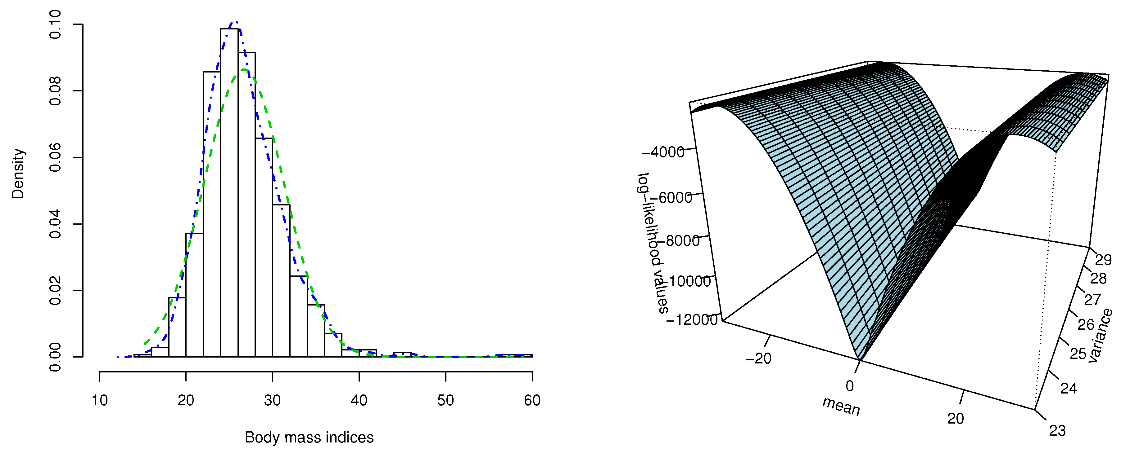
5. Application to Body Mass Index Data

6. Discussion
Conflicts of Interest
References
- Leone, F.C.; Nelson, L.S.; Nottingham, R.B. The folded normal distribution. Technometrics 1961, 3, 543–550. [Google Scholar] [CrossRef]
- Lin, H.C. The measurement of a process capability for folded normal process data. Int. J. Adv. Manuf. Technol. 2004, 24, 223–228. [Google Scholar] [CrossRef]
- Chakraborty, A.K.; Chatterjee, M. On multivariate folded normal distribution. Sankhya 2013, 75, 1–15. [Google Scholar] [CrossRef]
- Elandt, R.C. The folded normal distribution: Two methods of estimating parameters from moments. Technometrics 1961, 3, 551–562. [Google Scholar] [CrossRef]
- Johnson, N.L. The folded normal distribution: Accuracy of estimation by maximum likelihood. Technometrics 1962, 4, 249–256. [Google Scholar] [CrossRef]
- Johnson, N.L. Cumulative sum control charts for the folded normal distribution. Technometrics 1963, 5, 451–458. [Google Scholar] [CrossRef]
- Sundberg, R. On estimation and testing for the folded normal distribution. Commun. Stat.-Theory Methods 1974, 3, 55–72. [Google Scholar] [CrossRef]
- Kim, H.J. On the ratio of two folded normal distributions. Commun. Stat.-Theory Methods 2006, 35, 965–977. [Google Scholar] [CrossRef]
- Liao, M.Y. Economic tolerance design for folded normal data. Int. J. Prod. Res. 2010, 48, 4123–4137. [Google Scholar] [CrossRef]
- Nelder, J.A.; Mead, R. A simplex method for function minimization. Comput. J. 1965, 7, 308–313. [Google Scholar] [CrossRef]
- Johnson, N.L; Kotz, S.; Balakrishnan, N. Continuous Univariate Distributions; John Wiley & Sons, Inc.: New York, NY, USA, 1994. [Google Scholar]
- Psarakis, S.; Panaretos, J. The folded t distribution. Commun. Stat.-Theory Methods 1990, 19, 2717–2734. [Google Scholar] [CrossRef]
- Psarakis, S.; Panaretos, J. On some bivariate extensions of the folded normal and the folded t distributions. J. Appl. Stat. Sci. 2000, 10, 119–136. [Google Scholar]
- Kullback, S. Information Theory and Statistics; Dover Publications: New York, NY, USA, 1977. [Google Scholar]
- R Development Core Team. R: A Language and Environment for Statistical Computing. 2012. Available online: http://www.R-project.org/ (accessed on 1 December 2013).
- Yee, T.W. The VGAM package for categorical data analysis. J. Stat. Softw. 2010, 32, 1–34. [Google Scholar]
- Efron, B.; Tibshirani, R. An Introduction to the Bootstrap; Chapman and Hall/CRC: New York, NY, USA, 1993. [Google Scholar]
- MacMahon, S.; Norton, R.; Jackson, R.; Mackie, M.J.; Cheng, A.; Vander Hoorn, S.; Milne, A.; McCulloch, A. Fletcher challenge-university of Auckland heart and health study: Design and baseline findings. N. Zeal. Med. J. 1995, 108, 499–502. [Google Scholar]
© 2014 by the authors; licensee MDPI, Basel, Switzerland. This article is an open access article distributed under the terms and conditions of the Creative Commons Attribution license (http://creativecommons.org/licenses/by/3.0/).
Share and Cite
Tsagris, M.; Beneki, C.; Hassani, H. On the Folded Normal Distribution. Mathematics 2014, 2, 12-28. https://doi.org/10.3390/math2010012
Tsagris M, Beneki C, Hassani H. On the Folded Normal Distribution. Mathematics. 2014; 2(1):12-28. https://doi.org/10.3390/math2010012
Chicago/Turabian StyleTsagris, Michail, Christina Beneki, and Hossein Hassani. 2014. "On the Folded Normal Distribution" Mathematics 2, no. 1: 12-28. https://doi.org/10.3390/math2010012
APA StyleTsagris, M., Beneki, C., & Hassani, H. (2014). On the Folded Normal Distribution. Mathematics, 2(1), 12-28. https://doi.org/10.3390/math2010012