A High-Breakdown MCD-Based Robust Concordance Correlation Coefficient

Abstract

The concordance correlation coefficient (CCC) is a popular measure of agreement between two continuous variables but is highly sensitive to outliers and data contamination. In this study, we propose a robust reformulation of the CCC by replacing classical moment estimators with Minimum Covariance Determinant (MCD) estimators. The proposed robust CCC preserves the interpretability of the classical coefficient while providing substantially improved robustness. Comprehensive Monte Carlo simulations under normal and non-normal distributions, varying sample sizes, correlation levels, and contamination schemes compare the proposed coefficient with the classical CCC and existing robust alternatives. The results show that the proposed robust CCC achieves superior stability and accuracy in contaminated settings while remaining competitive under clean data. Theoretical properties of the estimator are discussed, and its practical usefulness is demonstrated using real glucose measurement and blood pressure data sets. The proposed method is implemented in the MVTests R package, enabling straightforward application to real-world data.

1. Introduction

The comparison of quantitative measurements requires assessing the extent to which different methods, devices, or observers can record the same value in an interchangeable manner. For this purpose, the Pearson product–moment correlation coefficient $\left(\rho \right)$ is frequently used to measure the strength of the linear relationship between two variables. When data points cluster tightly around a straight line, the correlation $\rho$ approaches 1. However, Pearson correlation $\rho$ does not account for systematic differences (bias) or scale discrepancies. For example, suppose two devices measuring TSH values are highly linearly related such as $y = 2x + 10$. Even if $\rho$ is close to 1, when device-X records a TSH value of 3, device-Y may record 16, leading to severe bias. Thus, a high $\rho$ does not guarantee absolute agreement or interchangeability between methods.

To address this limitation, Lin [1] proposed the concordance correlation coefficient (CCC), which simultaneously considers both precision and accuracy. The CCC is defined in Equation (1).

$${\rho }_C=1-{\displaystyle \frac{E\left[{\left(X-Y\right)}^2\right]}{E_{indep}\left[{\left(X-Y\right)}^2\right]}}={\displaystyle \frac{2{\sigma }_{XY}}{{\sigma }_X^2+{\sigma }_Y^2+{\left({\mu }_X-{\mu }_Y\right)}^2}}={\displaystyle \frac{2\rho {\sigma }_X{\sigma }_Y}{{\sigma }_X^2+{\sigma }_Y^2+{\left({\mu }_X-{\mu }_Y\right)}^2}}=\rho C_b$$

(1)

where $C_b={\displaystyle \frac{2{\sigma }_X{\sigma }_Y}{{\sigma }_X^2+{\sigma }_Y^2+{\left({\mu }_X-{\mu }_Y\right)}^2}}$, $E_{indep}$ is the expected value under the assumption that the variables X and Y are independent. The CCC measures the degree of agreement between two raters around the equality line $\left(y=x\right)$ in a scatterplot. In Equation (1), the term ${\left({\mu }_X-{\mu }_Y\right)}^2$ represents a measure of bias between the two raters, while ${\sigma }_X^2$ and ${\sigma }_Y^2$ express the scale differences. Therefore, the agreement between the two variables is penalized as the bias and scale differences increase. The Pearson correlation coefficient focuses solely on the strength of the linear association between two variables. By contrast, the concordance correlation coefficient assesses the degree to which two measurements are in absolute agreement and therefore interchangeable [1,2].

The key distinction between Pearson correlation and CCC is illustrated in Figure 1. In Figure 1, the red dashed line represents the equality line $\left(y=x\right)$, while the blue line corresponds to the OLS regression line. In Figure 1, Pearson correlation becomes high when the points lie close to the blue line. On the other hand, CCC becomes high when they cluster near the red equality line. In scenario (A), both $\rho$ and CCC are large since the two methods yield compatible results. However, in scenario (B), method Y consistently records higher values than method X. For this reason, $\rho$ yields a high despite systematic bias. Since interchangeability does not hold, the points deviate from the equality line $\left(y=x\right)$. Therefore, the CCC is relatively smaller.

Lin [1] further demonstrated that the CCC is asymptotically normally distributed and defined the Z transformation given in Equation (2).

$$\widehat{Z}={\displaystyle \frac{1}{2}}ln\left({\displaystyle \frac{1+{\widehat{\rho }}_C}{1-{\widehat{\rho }}_C}}\right)$$

(2)

Since its introduction, CCC has attracted substantial attention, particularly in the medical sciences [3,4,5,6,7,8]. Applications often involve the evaluation of agreement between diagnostic markers, measurement devices, or raters. In addition, several methodological developments have been made: Lin [2] discussed the use of CCC in assay validation and provided guidelines for sample size and power analysis; King and Chinchilli [9] generalized CCC to both continuous and categorical data; King, et al. [10] and Carrasco, et al. [11] extended CCC to repeated measurements; Williamson, et al. [12] proposed a resampling-based hypothesis testing approach; Feng, et al. [13] proposed jackknife confidence intervals for ${\rho }_C$, and Feng, et al. [14] compared several confidence intervals.

Nevertheless, the vulnerability of the classical CCC to outliers has been widely emphasized in the literature. Because CCC relies on moment-based estimators of means, variances, and covariances, it becomes unreliable under heavy-tailed distributions, skewed structures, or contamination. To mitigate this problem, King and Chinchilli [15] reformulated Equation (1) as in Equation (3):

$${\rho }_g={\displaystyle \frac{\left[E_{F_X{F}_Y}g\left(X-Y\right)-E_{F_X{F}_Y}g\left(X+Y\right)\right]-\left[E_{F_{XY}}g\left(X-Y\right)-E_{F_{XY}}g\left(X+Y\right)\right]}{E_{F_X{F}_Y}g\left(X-Y\right)-E_{F_X{F}_Y}g\left(X+Y\right)+\frac{1}{2}{E}_{F_X}g\left(2X\right)+\frac{1}{2}{E}_{F_Y}g\left(2Y\right)}}$$

(3)

where $E_{F_X{F}_Y}g\left(.\right)$ is the expected value of the function g under $F_{XY}(.)=F_X(.)F_Y(.)$, $F_{XY}$ is the cumulative distribution function (cdf) of the bivariate population for pairs $(X_i,Y_i)$, $F_X$ and $F_Y$ are the marginal distribution functions of X and Y, respectively.

The function $g\left(z\right)$ must satisfy the following conditions:

• $g\left(0\right)=0$,
• $g(-z)=g\left(z\right)$ for all z,
• g(z) is nondecreasing function of z for all z ≥ 0.

King and Chinchilli [15] proposed five candidate functions meeting these conditions:

(a)

$g_1(z)=z^2$ for the squared distance function (classical CCC),

(b)

$g_2(z)=\left\{\begin{array}{c}{z}^2, \left|z\right|\le z_0\\ z_0^2, \left|z\right|>z_0\end{array}\right.$ for Winsorized squared distance function,

(c)

$g_3(z)={\left|z\right|}^{\delta }$, where $1\le \delta \le 2$, for the absolute distance function,

(d)

$g_4(z)=\left\{\begin{array}{c}{\left|z\right|}^{\delta }, \left|z\right|\le z_0\\ {\left|z_0\right|}^{\delta }, \left|z\right|>z_0\end{array}\right.$ for Winsorized absolute distance function,

(e)

$g_5(z)=\left\{\begin{array}{c}{z}^2/2 , \left|z\right|\le z_0\\ z_0\left|z\right|-z_0^2/2, \left|z\right|>z_0\end{array}\right.$ for Huber’s function.

Here, $z_0>0$ is a constant selected. Function (a) corresponds to the classical CCC, whereas functions (b)–(e) define robust CCC variants. King and Chinchilli [15] showed that these robust CCC estimators achieve smaller errors at moderate contamination levels (10–25%).

Another important robust extension of the concordance correlation coefficient is the robust Bayesian CCC, proposed by Feng, et al. [16]. In this approach, robustness is achieved by modelling the joint distribution of paired measurements using a multivariate Student’s t-distribution instead of a Gaussian distribution, thereby naturally downweighing extreme observations through heavy-tailed behaviour. Under this framework, the CCC is defined as

$${\rho }_{Bayes}={\displaystyle \frac{2\sum _{i=1}^{d-1}\sum _{j=i+1}^d\frac{\nu }{\nu -2}{\sigma }_{ij}}{\left(d-1\right)\sum _{i=1}^d\frac{\nu }{\nu -2}{\sigma }_i^2+\sum _{i=1}^{d-1}\sum _{j=i+1}^d{\left({\mu }_i-{\mu }_j\right)}^2}}$$

(4)

where $\nu$ is the degrees of freedom, ${\mu }_i$’s are components of the location vector, ${\sigma }_i^2$’s are diagonal elements of the scale matrix, and ${\sigma }_{ij}$’s are off-diagonal elements of the scale matrix. As $\nu \to \mathrm{\infty }$, the multivariate t-distribution converges to the normal distribution, and the Bayesian CCC reduces to the classical CCC. By embedding the CCC within a Bayesian framework, this method enables posterior inference, credible intervals, and the incorporation of covariates or repeated measurements. Simulation studies and real data applications have shown that the robust Bayesian CCC is less sensitive to outliers and deviations from normality than classical moment-based estimators. Nevertheless, the approach relies on parametric distributional assumptions and Markov chain Monte Carlo estimation, which may increase computational cost and limit scalability in large-sample or high-dimensional settings [16].

In addition to M-estimation–based approaches, Vallejos, et al. [17] proposed an alternative robust formulation of the concordance correlation coefficient based on L1-type loss functions, which replaces the squared distance used in the classical CCC with absolute deviations. The resulting L1-based concordance coefficient, given in Equation (5), measures agreement by normalizing the expected absolute difference between paired observations relative to the case of independence.

$${\rho }_{L1}={\displaystyle \frac{E\left(\left|X_1-X_2\right|\right)}{E\left(\left|X_1-X_2\right| | {\sigma }_{12}=0\right)}}.$$

(5)

By relying on absolute differences, the L1-based CCC reduces the influence of extreme observations and heavy-tailed distributions, offering increased robustness compared to moment-based estimators. This formulation is particularly effective in situations where marginal outliers distort second-order moments. However, since robustness is achieved through a univariate distance measure, the L1-based CCC primarily addresses marginal deviations and does not explicitly account for the joint multivariate structure of the data, which may limit its effectiveness under complex or multivariate contamination patterns [17]. In our study, these robust CCC variants are used as benchmarks for comparison with the proposed estimator.

Finally, some studies have also explored the use of CCC in longitudinal data with missing and contaminated observations, combining robust covariance estimators with imputation strategies [18].

In this study, we introduce a robust alternative to the classical CCC that provides reliable estimates in contaminated data without being distorted by outliers. The methodological details of the proposed estimator are presented in Section 2. Section 3 reports an extensive simulation study evaluating its performance, while Section 4 demonstrates its practical utility using a real dataset. Section 5 describes the R functions developed for implementation, and Section 6 concludes with a discussion of the findings.

2. Proposed Robust Concordance Correlation Coefficients (RCCC)

2.1. Motivation

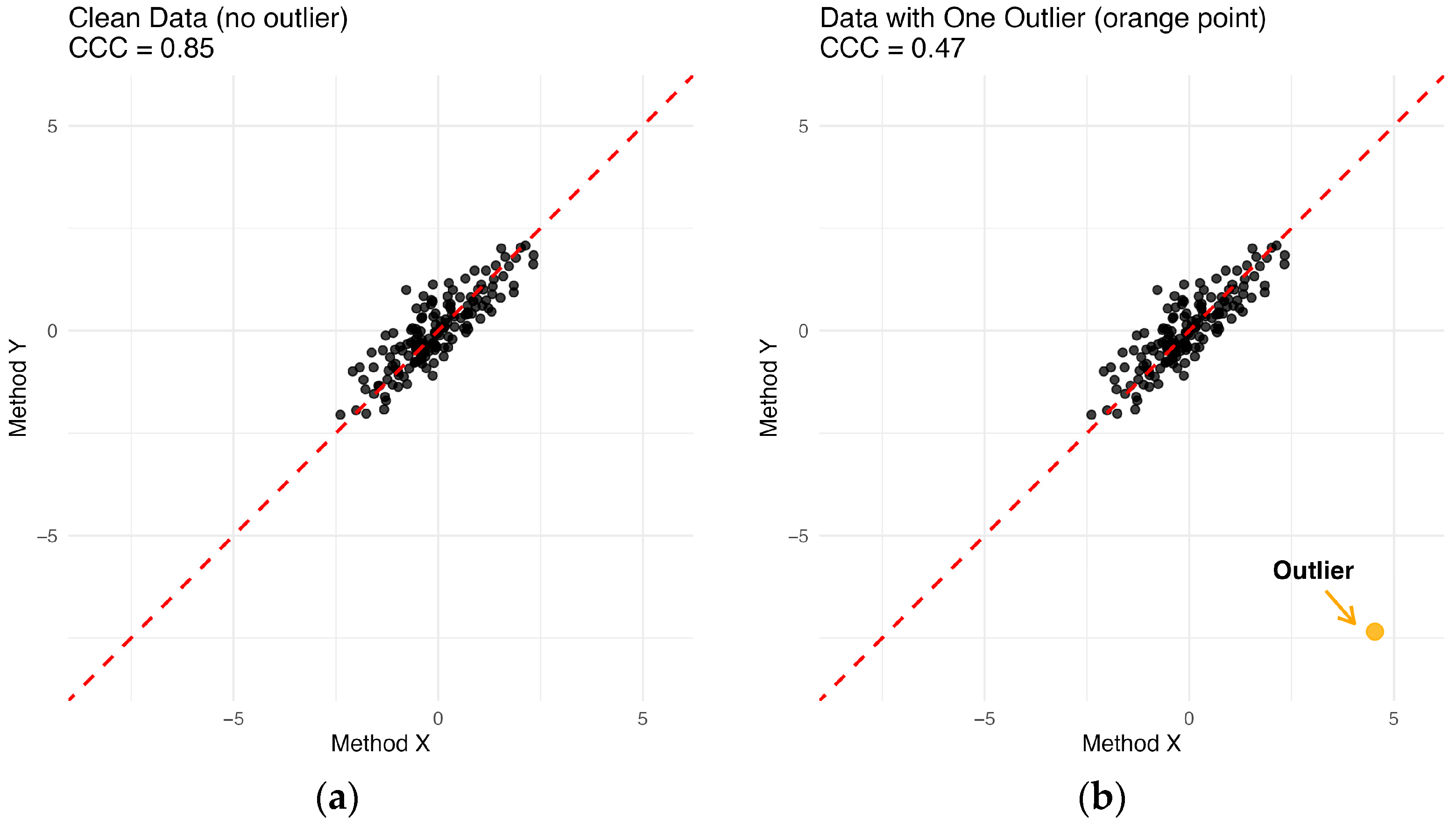
When data contain outliers, the CCC defined in Equation (1) can yield misleading results, primarily because it relies on classical mean, variance, and covariance estimators that are sensitive to contamination. This problem is illustrated in Figure 2. In Figure 2a, the points cluster tightly around the equality line, yielding a CCC of 0.85. However, after adding just a single outlier, the CCC drops dramatically to 0.47, despite the majority of points still lying close to the equality line. This illustrates the lack of robustness of CCC, and underscores the need for a robust concordance correlation coefficient.

Although, King and Chinchilli [15] suggested using alternative functions instead of the squared function to provide resistance against outliers, the performance of their coefficients depend on the choice of function, and this performance varies according to the selection of the constant ${\mathit{z}}_{\mathbf{0}}$. Similarly, L1-based concordance measures was proposed to reduce sensitivity to extreme observations by replacing the quadratic loss with an absolute deviation criterion; however, this comes at the cost of reduced efficiency under clean data and may lead to unstable behavior when the underlying distributions deviate from symmetry [17]. Finally, Feng, Baumgartner and Svetnik [16] suggested Robust Bayesian concordance approaches, on the other hand, achieve resistance to outliers by introducing heavy-tailed distributions and hierarchical modeling assumptions. While effective in many settings, their performance depends on prior specifications, fixed degrees-of-freedom parameters, and computational complexity, which may limit their practical applicability and reproducibility.

These limitations collectively motivate the development of a new robust concordance correlation coefficient that preserves high efficiency under clean data while providing stable and reliable performance in the presence of contamination, without relying on tuning constants, strong distributional assumptions, or intensive computational procedures.

2.2. Definition

Let $\left(X_i,Y_i\right)(i=\mathrm{1,2},...,n)$ be pairs drawn from an arbitrary bivariate distribution with joint distribution function $F_{XY}\left(x,y\right)$, with mean vector $\mathit{\mu }={\left[{\mu }_{\mathit{X}},{\mu }_{\mathit{Y}}\right]}^{\mathit{T}}$ and covariance matrix $\mathit{\Sigma }=\left[\begin{array}{cc}{\sigma }_{\mathit{X}}^{\mathbf{2}}& {\sigma }_{XY}\\ {\sigma }_{YX}& {\sigma }_{\mathit{Y}}^{\mathbf{2}}\end{array}\right]$. The population concordance correlation coefficient (CCC) is defined as ${\rho }_C{\displaystyle \frac{2{\sigma }_{XY}}{{\sigma }_X^2+{\sigma }_Y^2+{\left({\mu }_X-{\mu }_Y\right)}^2}}$. When classical estimations of these parameters are used in this expression, CCC may be sensitive to contamination. To obtain robust CCC while preserving its form, we propose to replace the classical mean and covariance estimations with their Minimum Covariance Determinant (MCD) ones.

Intuitively, the robustness of the Minimum Covariance Determinant estimator stems from its focus on the most homogeneous subset of the data rather than the full sample. Instead of being influenced by all observations, including extreme or contaminated points, the MCD identifies the subset with the smallest covariance determinant, which corresponds to the core data cloud. As a result, observations lying far from the main data structure receive little or no influence on the estimated location and scatter, making MCD-based estimators naturally resistant to outliers and contamination.

For a trimming level $h\in \left\{⌈n/2⌉,...,n\right\}$, consider all index subsets $H$ of size $h$. For each $H$, let us define

• the subset mean ${\widehat{\mathit{\mu }}}_H={\displaystyle \frac{1}{h}}\sum _{i\in H}{\mathit{z}}_i$ with $\mathit{z}\mathrm{ᵢ}={\left[X\mathrm{ᵢ},Y\right]}^{\mathit{T}}$,
• the subset covariance ${\widehat{\mathit{\Sigma }}}_H={\displaystyle \frac{1}{(h-1)}}\sum _{i\in H}{\left[{\mathit{z}}_i-{\widehat{\mathit{\mu }}}_H\right]\left[{\mathit{z}}_i-{\widehat{\mathit{\mu }}}_H\right]}^T$.

where, ${\left[.\right]}^{\mathit{T}}$ is transpose operator.

The MCD estimator selects the subset $H^{\mathrm{*}}$ that minimizes det $\left({\mathit{S}}_H\right)$ over all such $H$. The MCD location and scatter estimators are then ${\widehat{\mathit{\mu }}}_{MCD}={\widehat{\mathit{\mu }}}_{H^{\mathrm{*}}}$ and ${\widehat{\mathit{\Sigma }}}_{MCD}={\widehat{\mathit{\Sigma }}}_{H^{\mathrm{*}}}$ [19].

According to this definition, the MCD estimates of the mean vector and covariance matrix of the bivariate distribution from which the pairs $\left(X_i,Y_i\right)(i=\mathrm{1,2},...,n)$ are drawn can then be expressed as in Equation (6):

$${\widehat{\mathit{\mu }}}_{MCD}=\left[\begin{array}{c}{\widehat{\mu }}_{X.MCD}\\ {\widehat{\mu }}_{Y.MCD}\end{array}\right],{\widehat{\mathit{\Sigma }}}_{MCD}=\left[\begin{array}{cc}{\widehat{\sigma }}_{X.MCD}^2& {\widehat{\sigma }}_{XY.MCD}\\ {\widehat{\sigma }}_{YX.MCD}& {\widehat{\sigma }}_{Y.MCD}^2\end{array}\right]$$

(6)

Let $\alpha =1-h/n$ denote the trimming proportion. The breakdown point of MCD estimations equals $\alpha$ and attains its maximum near 50% when $h\approx n/2$, providing high resistance to outliers [20].

As a result, in this study we propose replacing the classical mean, variance, and covariance terms in the concordance correlation coefficient ${\rho }_C$ given in Equation (1) with MCD estimators, leading to the robust concordance correlation coefficient $\left({\rho }_R\right)$ defined in Equation (7):

$${\rho }_R={\displaystyle \frac{2{\widehat{\sigma }}_{XY.MCD}}{{\widehat{\sigma }}_{X.MCD}^2+{\widehat{\sigma }}_{Y.MCD}^2+{\left({\widehat{\mu }}_{X.MCD}-{\widehat{\mu }}_{Y.MCD}\right)}^2}}$$

(7)

On clean data, the robust and classical summaries coincide and ${\rho }_R$ reduces to the usual sample ${\rho }_C$; under contamination, ${\rho }_R$ remains stable while retaining the interpretability of ${\rho }_C$. Since ${\rho }_R$ is based on MCD estimators with a high breakdown point, it is resistant to outliers. Thus, the proposed coefficient avoids misleading assessments such as the one illustrated in Figure 2b when outliers are present. The performance of the proposed measure is demonstrated through both simulation studies and a real data application.

2.3. Range and Affine Invariance Properties of ${\mathit{\rho }}_{\mathit{R}}$

This subsection establishes that the proposed robust concordance correlation coefficient $\left({\rho }_R\right)$ is well-defined under mild conditions and is bounded within the closed interval [−1, 1]. We further characterize equality conditions, degenerate cases (such as zero variance), and invariance properties that are relevant for practical applications.

Let us define the denominator $D={\widehat{\sigma }}_{X.MCD}^2+{\widehat{\sigma }}_{Y.MCD}^2+{\left({\widehat{\mu }}_{X.MCD}-{\widehat{\mu }}_{Y.MCD}\right)}^2\ge 0$ and the proposed coefficient ${\rho }_R=2{\widehat{\sigma }}_{XY.MCD}/D$.

Lemma 1. 

The robust CCC $\left({\rho }_R\right)$ lies in the closed interval [−1, 1]:

$$-1\le {\rho }_R\le 1$$

(8)

Proof of Lemma 1. 

By Cauchy–Schwarz (C-S) inequality, we can write $\left|{\widehat{\sigma }}_{XY.MCD}\right|\le \sqrt{{\widehat{\sigma }}_{X.MCD}^2\times {\widehat{\sigma }}_{Y.MCD}^2}$. Moreover, by the Arithmetic Mean–Geometric Mean (AM-GM) inequality, we know $\sqrt{ab}\le \left(a+b\right)/2$ for any $a,b\ge 0$. Combining these properties, we obtain

$$\left|{\widehat{\sigma }}_{XY.MCD}\right|\le \sqrt{{\widehat{\sigma }}_{X.MCD}^2\times {\widehat{\sigma }}_{Y.MCD}^2}\le {\displaystyle \frac{{\widehat{\sigma }}_{X.MCD}^2+{\widehat{\sigma }}_{Y.MCD}^2}{2}}\le {\displaystyle \frac{{\widehat{\sigma }}_{X.MCD}^2+{\widehat{\sigma }}_{Y.MCD}^2}{2}}$$

Because ${\left({\widehat{\mu }}_{X.MCD}-{\widehat{\mu }}_{Y.MCD}\right)}^2\ge 0$, we can write;

$$\left|{\widehat{\sigma }}_{XY.MCD}\right|\le {\displaystyle \frac{{\widehat{\sigma }}_{X.MCD}^2+{\widehat{\sigma }}_{Y.MCD}^2+{\left({\widehat{\mu }}_{X.MCD}-{\widehat{\mu }}_{Y.MCD}\right)}^2}{2}}={\displaystyle \frac{D}{2}}$$

Therefore,

$$\left|{\widehat{\sigma }}_{XY.MCD}\right|\le {\displaystyle \frac{D}{2}}.$$

If we multiply the last inequality by 2 and divide by $D$:

$$\left|{\rho }_R\right|={\displaystyle \frac{2\left|{\widehat{\sigma }}_{XY.MCD}\right|}{D}}\le 1$$

then

$$-1\le {\rho }_R\le 1$$

□

If ${\widehat{\mu }}_{X.MCD}={\widehat{\mu }}_{Y.MCD}$ and ${\widehat{\sigma }}_{X.MCD}^2={\widehat{\sigma }}_{Y.MCD}^2=\left|{\widehat{\sigma }}_{XY.MCD}\right|$, then $\left|{\rho }_R\right|=1$. In finite samples these conditions are rarely met exactly; hence $\left|{\rho }_R\right|<1$ typically holds.

The denominator D is always nonnegative by construction. If both robust marginal variances ${\widehat{\sigma }}_{X.MCD}^2={\widehat{\sigma }}_{Y.MCD}^2=0$ and robust means ${\widehat{\mu }}_{X.MCD}={\widehat{\mu }}_{Y.MCD}=0$, then $D = 0$, corresponding to a degenerate sample with no variation and perfect equality, ${\rho }_R$ is indeterminate $(0/0)$. In practice, this occurs only if X and $Y$ are both constant (after robust trimming). If exactly one variance is zero, then ${\widehat{\sigma }}_{XY.MCD}=0$ as well (since covariance with a constant is zero), whence ${\widehat{\rho }}_R=0$. Thus, outside fully degenerate scenarios $(D = 0)$, ${\rho }_R$ is well-defined and bounded.

Because the MCD estimator is affine equivariant, the proposed ${\rho }_R$ is affine invariant. In particular, translating $X$ and $Y$ by constants or multiplying both by the same positive factor leaves ${\widehat{\rho }}_R$ unchanged. Opposite sign rescalings flip the sign consistently with correlation. These properties parallel those of the classical ${\rho }_C$.

Taken together, these results ensure that ${\rho }_R$ is well-defined outside fully degenerate samples and bounded in [−1, 1]. Moreover, because the MCD location and scatter estimators are affine equivariant, the resulting concordance measure ${\rho }_R$ is affine invariant: under common affine transformations applied to both variables (e.g., joint translations and positive rescalings), its value remains unchanged (with sign changes behaving consistently under sign reversals). In addition, since MCD attains a high breakdown point for location and scatter, ${\rho }_R$ inherits strong stability under substantial contamination through its robust inputs. These theoretical properties underpin the robust performance patterns observed in the simulation study.

3. Simulation Study

In this study, a comprehensive Monte Carlo simulation was conducted to compare the performance of the concordance correlation coefficient (CCC) proposed by Lin [1], the robust CCC estimators based on alternative $g\left(.\right)$ functions [15], Bayes approach [16], L1 estimations [17], and the proposed robust CCC (rCCC) based on Minimum Covariance Determinant (MCD) estimators. The simulation was carried out for three different population correlation coefficients $\left(\rho =0.45, 0.6, 0.9\right)$ and five different sample sizes $\left(n=30, 50, 100, 200, 500\right)$ in each scenario. Assuming that the variables X and Y follow a bivariate distribution, data were generated under clean conditions using five different distributional/design combinations.

• Design A: Random observations were drawn from the bivariate normal distribution $\left[\begin{array}{c}X\\ Y\end{array}\right]~N_2\left(\left[\begin{array}{c}0\\ 0\end{array}\right],\left[\begin{array}{cc}1& \rho \\ \rho & 1\end{array}\right]\right)$. Here, the two variables have identical locations and scales.
• Design B: Random observations were drawn from the bivariate normal distribution $\left[\begin{array}{c}X\\ Y\end{array}\right]~N_2\left(\left[\begin{array}{c}0\\ 0\end{array}\right],\left[\begin{array}{cc}1& 2\rho \\ 2\rho & 4\end{array}\right]\right)$. Here, the two variables have identical locations but different scales.
• Design C: Random observations were drawn from the bivariate normal distribution $\left[\begin{array}{c}X\\ Y\end{array}\right]~N_2\left(\left[\begin{array}{c}0\\ 2\end{array}\right],\left[\begin{array}{cc}1& \rho \\ \rho & 1\end{array}\right]\right)$. Here, the two variables have identical scales but different locations.
• Design D: In this design, random observations are initially generated from Design A and subsequently subjected to an exponential transformation, yielding variables with a log-normal distribution.
• Design E: Random observations were drawn from a multivariate t distribution with degrees of freedom $df=5$ and covariance matrix $\left[\begin{array}{cc}1& \rho \\ \rho & 1\end{array}\right]$

Designs D and E were chosen to examine the performance of the coefficients under skewed and heavy-tailed distributions.

In each simulation design, the population value of the CCC $\left({\rho }_C\right)$ defined by Lin [1] is expressed in terms of the parameter $\rho$, which was used as the measure of association in the simulation, as given in

Table 1. Population concordance ${\rho }_c$ corresponding to the design parameter $\rho$.

Design	${\mathit{\rho }}_{\mathit{c}}$
A	$\rho$
B	$0.8\rho$
C	$\rho /3$
D	$\left(e^{\rho }-1\right)/\left(e-1\right)$
E	$\rho$

(full derivations in Appendix A):

For each design, the value of the parameter ${\rho }_C$ was calculated based on the population correlation values $\rho \left(0.45, 0.6, 0.9\right)$, and this value was taken as the ‘true’ concordance correlation coefficient. Subsequently, from the corresponding populations, 3000 random samples of sizes $n$ $\left(30, 50, 100, 200, 500\right)$ were drawn for each scenario and combination, and eight different estimators $\left({\widehat{\rho }}_C,{\widehat{\rho }}_R,{\widehat{\rho }}_{g_2},{\widehat{\rho }}_{g_3},{\widehat{\rho }}_{g_4},{\widehat{\rho }}_{g_5},{\widehat{\rho }}_{L1},{\widehat{\rho }}_{Bayes}\right)$ were computed. The performance of these estimators was evaluated using the root mean square error (RMSE) values, calculated as in Equation (9).

$$RMSE=\sqrt{{\displaystyle \frac{1}{3000}}\sum _{i=1}^{3000}{\left({\rho }_C-{\widehat{\rho }}_i\right)}^2}$$

(9)

Here, instead of ${\widehat{\rho }}_i$, one of the estimators $\left({\widehat{\rho }}_C,{\widehat{\rho }}_R,{\widehat{\rho }}_{g_2},{\widehat{\rho }}_{g_3},{\widehat{\rho }}_{g_4},{\widehat{\rho }}_{g_5},{\widehat{\rho }}_{L1},{\widehat{\rho }}_{Bayes}\right)$ is used, and the RMSE of the selected estimator is calculated according to Equation (9).

3.1. Simulation Study for Clean Data

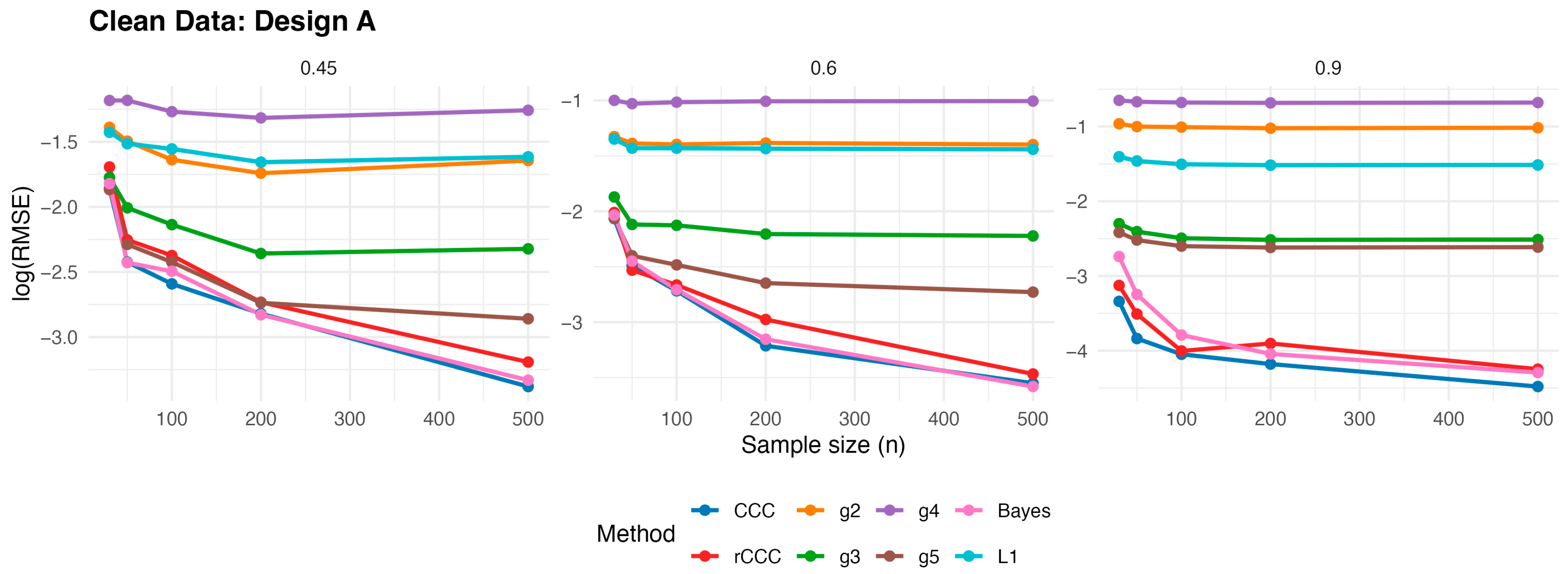
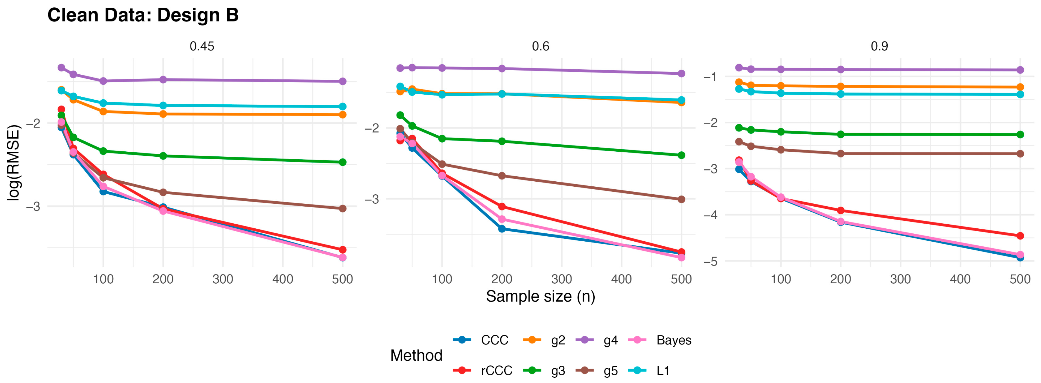
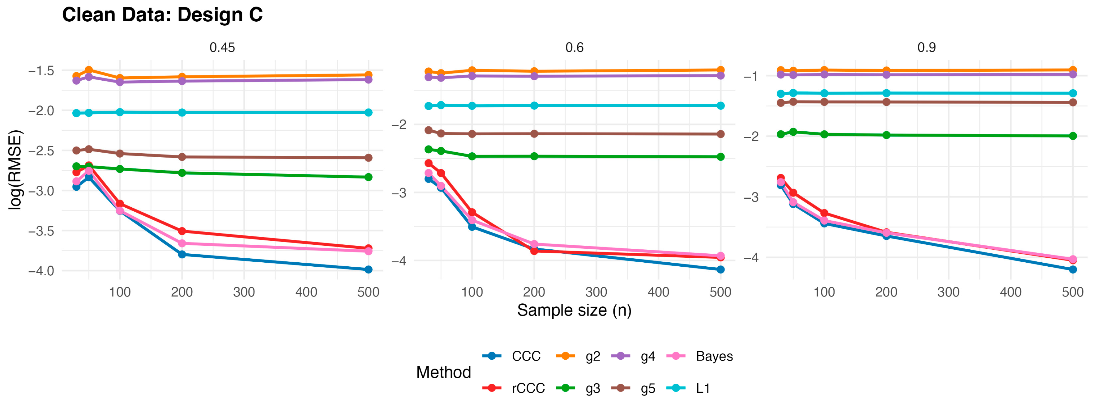
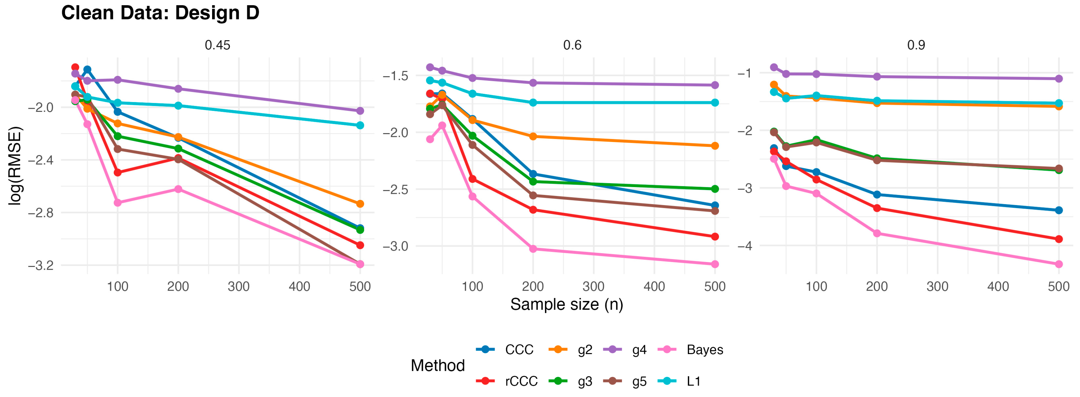
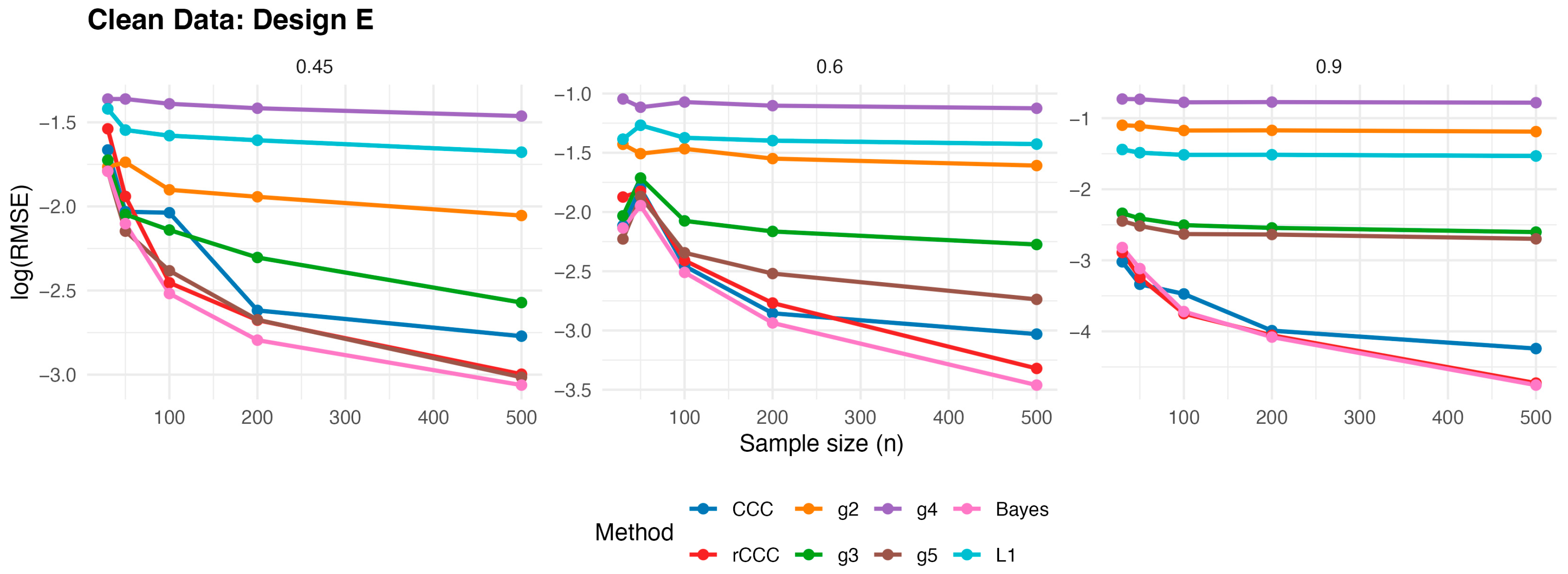
In this subsection, we randomly generate data for five different designs as previously described, and the RMSE values were computed for each case as given in Equation (9). For visualization purposes, Figure 3, Figure 4, Figure 5, Figure 6 and Figure 7 report the corresponding $log\left(RMSE\right)$ values to facilitate a clearer comparison across estimators with different error scales, whereas the exact RMSE values are provided in the Supplementary File Tables S1–S5.

According to Figure 3, Figure 4, Figure 5, Figure 6 and Figure 7, several consistent patterns emerge across all designs under clean data conditions. First, for all estimators, the error levels decrease monotonically as the sample size increases from 30 to 500, reflecting the expected consistency behaviour. This pattern is observed uniformly across all correlation levels and designs.

Second, stronger population correlations are associated with smaller error values. In all designs, the estimators exhibit noticeably lower $log\left(RMSE\right)$ when the true correlation is high $(\rho = 0.90)$ compared to weaker association levels $(\rho = 0.45)$, indicating improved agreement estimation as the underlying concordance increases.

Third, across all five designs, the proposed rCCC performs almost indistinguishably from the classical CCC in the absence of contamination. Their curves largely overlap in the graphical results, demonstrating that the proposed robust estimator does not suffer from efficiency loss under clean conditions. This behaviour holds not only under the standard bivariate normal setting, but also for skewed and heavy-tailed yet uncontaminated designs.

Fourth, the alternative robust concordance measures, including the g2–g5 variants of King and Chinchilli [15] as well as Bayes approach [16], L1 estimations [17], generally yield larger error levels in clean data. While some of these methods occasionally approach the performance of CCC and rCCC at large sample sizes or high correlations, they do not consistently outperform them and often exhibit reduced efficiency, particularly at lower correlations.

Finally, departures from normality alone—such as skewness or heavy tails without explicit outliers—do not alter the overall conclusions. In all clean designs, the classical CCC and the proposed rCCC remain the most efficient estimators, whereas the alternative robust methods provide no clear advantage in the absence of contamination. Overall, the clean-data simulations confirm that rCCC preserves the efficiency of CCC while retaining its robustness-oriented formulation.

3.2. Simulation Study for Unidirectional Contaminated Data

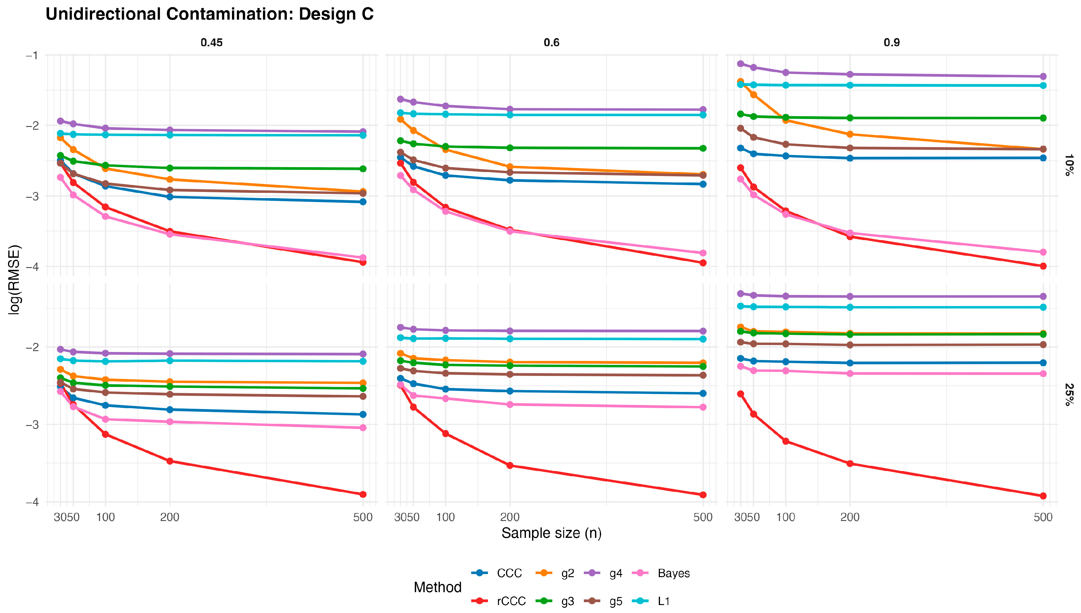
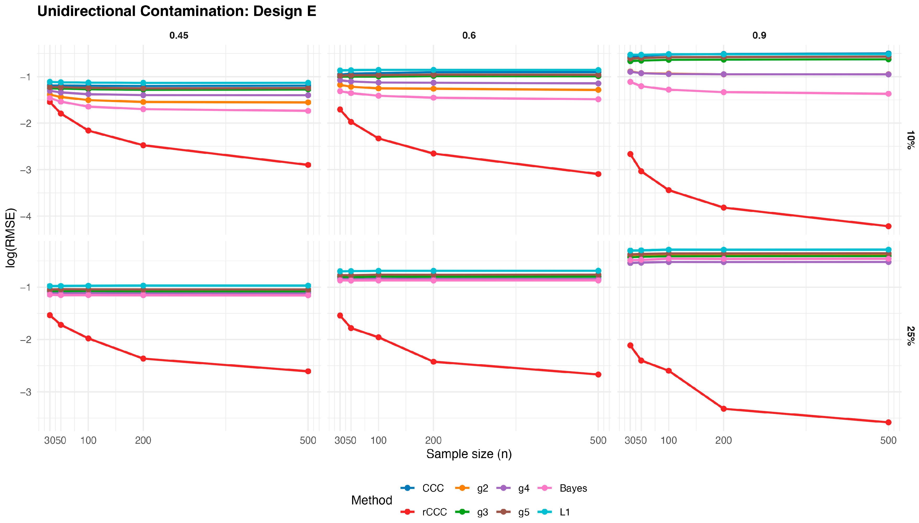
In this subsection, we investigated the performance of all concordance estimators under unidirectional contamination, where outliers affect only one of the variables. During the contamination process, random data were first generated cleanly according to the five different designs described in Section 3.1. Then, the X-values of the last $h=⌊n\times \epsilon ⌋$ observations in the dataset were multiplied by 10 to introduce contamination, where $n$ denotes the sample size and $\epsilon$ the contamination rate ($\epsilon =0.1, 0.25$). 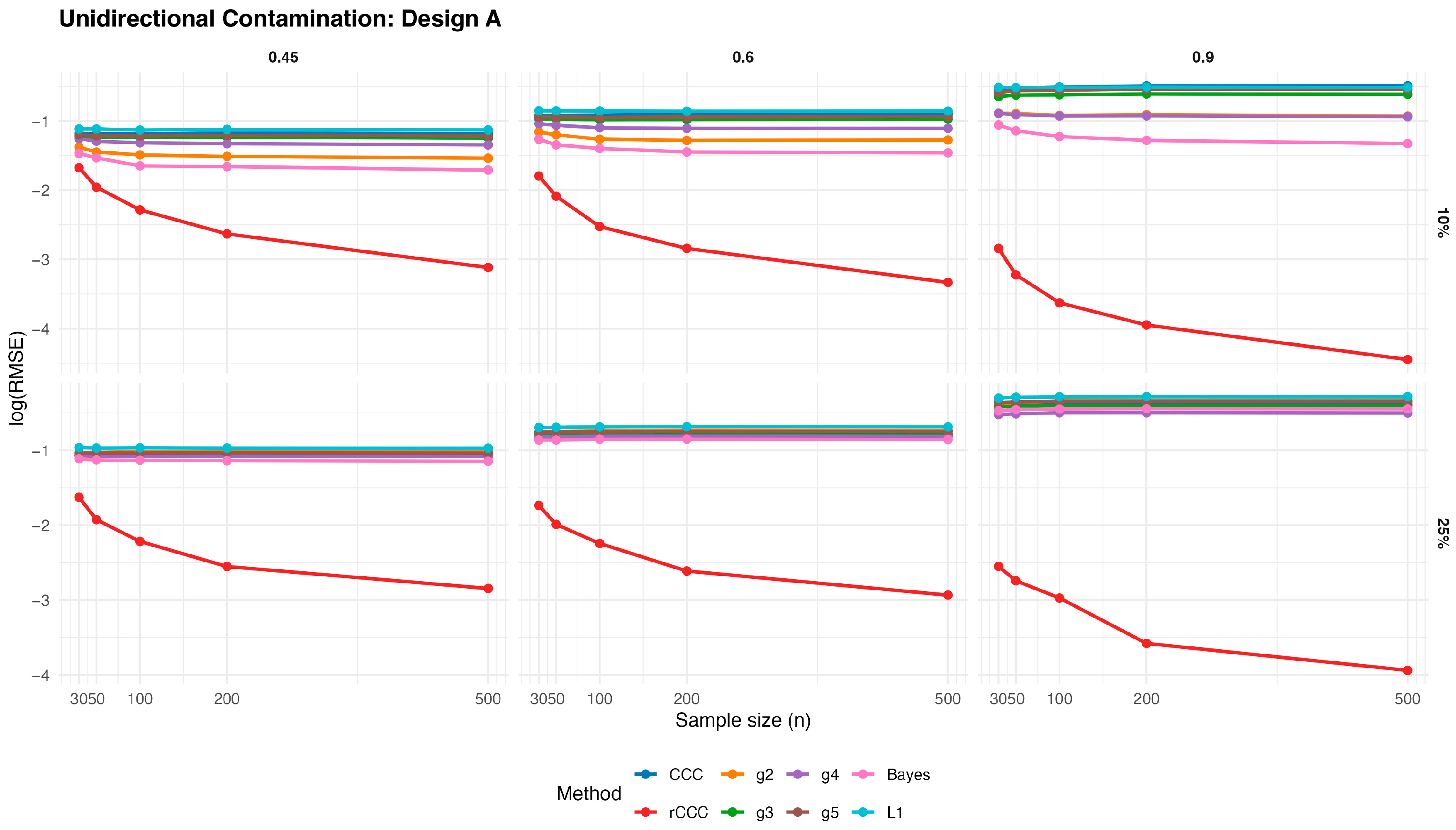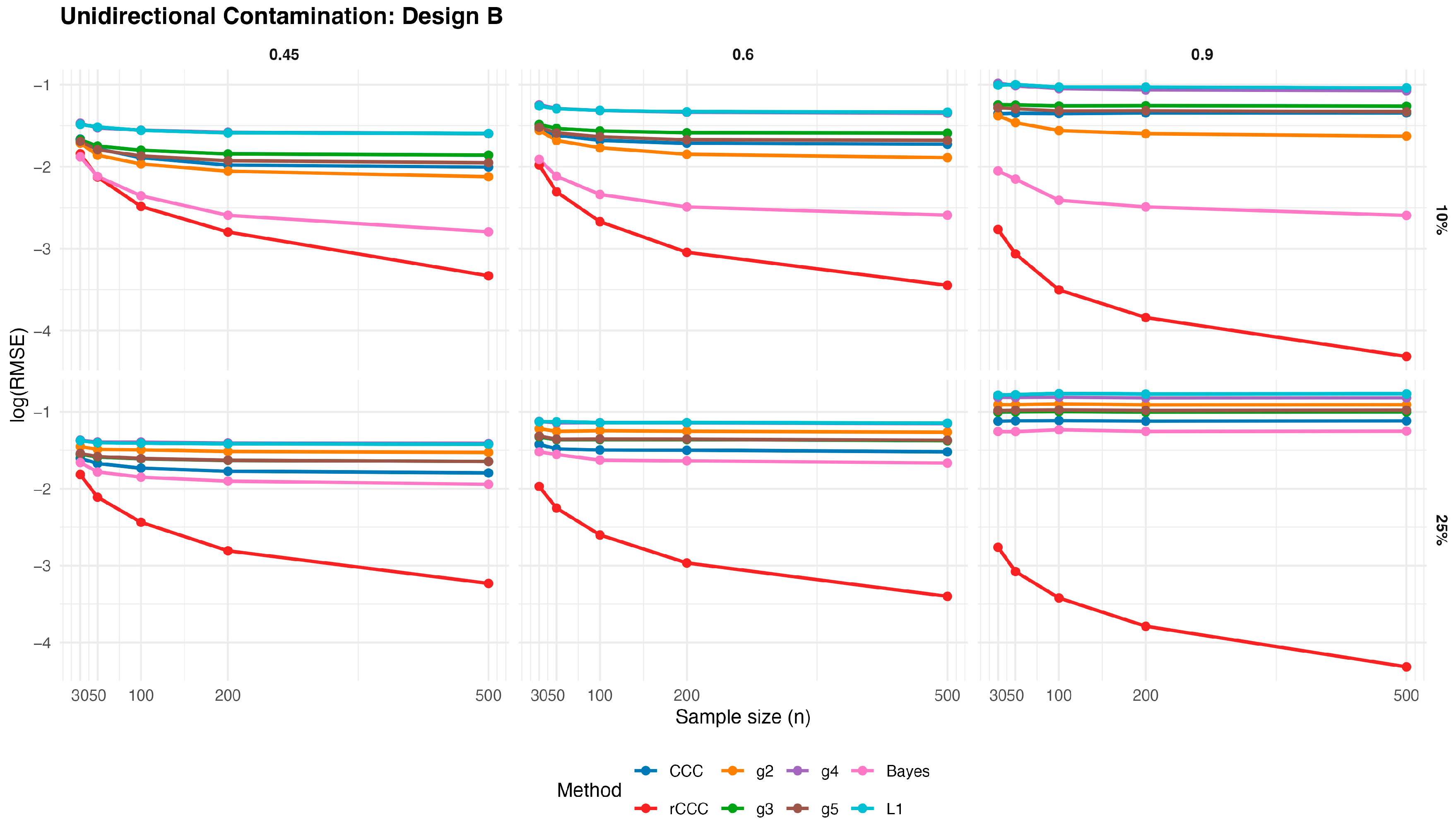The resulting RMSE values are reported in the Supplementary File Tables S6–S10, while graphical summaries are presented in Figure 8, Figure 9, Figure 10, Figure 11 and Figure 12.

According to these results, the classical CCC is highly sensitive to unidirectional contamination. As illustrated in Figure 8, Figure 9, Figure 10, Figure 11 and Figure 12, its $log\left(RMSE\right)$ values increase sharply once contamination is introduced. This deterioration is visible across all designs and becomes more pronounced as the contamination rate increases from 10% to 25%. Notably, increasing the sample size does not mitigate this effect, indicating that the classical CCC remains vulnerable even in large samples.

In contrast, the proposed MCD-based rCCC shows strong robustness. In Figure 8, Figure 9, Figure 10, Figure 11 and Figure 12, the rCCC curves remain relatively flat across different sample sizes and contamination levels. This pattern is consistent for all population concordance levels and across different distributional designs. The graphical results clearly demonstrate that the rCCC is largely unaffected by one-sided contamination.

The robust CCC variants proposed by King and Chinchilli (g2–g5) exhibit mixed behaviour. In the figures, some variants show partial improvement over the classical CCC, particularly at lower contamination levels. However, their $log\left(RMSE\right)$ curves display noticeable variability across designs and correlation levels. In several scenarios, these estimators show increasing error as contamination intensifies, and none achieves the consistent stability observed for the rCCC.

The L1-based concordance coefficient provides improved robustness relative to the classical CCC. As seen in Figure 8, Figure 9, Figure 10, Figure 11 and Figure 12, its error curves lie below those of the classical CCC in most scenarios. This improvement reflects the reduced sensitivity of absolute deviations to extreme observations. Nevertheless, the L1-based estimator still exhibits visible performance degradation as contamination increases, especially at higher correlation levels, suggesting limited protection against distortions in the joint dependence structure.

Similarly, the robust Bayesian CCC improves resistance to outliers through its heavy-tailed modelling framework. In the graphical results, it generally outperforms the classical CCC and shows smoother behaviour across sample sizes. However, its $log\left(RMSE\right)$ curves remain above those of the rCCC in most settings, and its performance becomes less stable under stronger contamination.

As expected, increasing the sample size leads to lower error levels for all estimators. This trend is clearly visible in Figure 8, Figure 9, Figure 10, Figure 11 and Figure 12. However, the relative ranking of the methods remains unchanged. Estimators that are sensitive to unidirectional contamination continue to exhibit higher error levels even for large samples.

Overall, the graphical evidence confirms that while several robust approaches—including L1-based and Bayesian CCCs—provide meaningful improvements over the classical CCC, the proposed MCD-based rCCC consistently delivers the most stable and reliable performance across all designs, contamination levels, and sample sizes.

3.3. Simulation Study for Bidirectional Contaminated Data

In order to investigate the behaviour of the competing estimators under more challenging contamination mechanisms, we consider a bidirectional contamination scheme, where entire observations are simultaneously corrupted in both variables. Let

$${\mathbf{Z}}_i=(X_i,Y_i{)}^{\mathrm{\top }},i=1,\dots ,n$$

(10)

denote a bivariate sample generated from the clean data-generating mechanism described in Section 3.1. For a given contamination rate $\epsilon \in \left\{0.10, 0.25\right\}$, we randomly select $m=\lceil \epsilon n\rceil$ observations and replace them with outlying values. The contaminated observations are generated independently from a bivariate normal distribution with shifted location and inflated dispersion,

$${\mathbf{Z}}_i^{\left(\mathrm{o}\mathrm{u}\mathrm{t}\right)}\sim {\mathcal{N}}_2\left(\left(\begin{array}{c}8\\ -8\end{array}\right),\left(\begin{array}{cc}9& 0\\ 0& 9\end{array}\right)\right)$$

(11)

which induces extreme values in both components. This construction produces rowwise contamination and naturally introduces leverage-type outliers, known to severely affect classical covariance- and concordance-based estimators.

For non-Gaussian designs, the same transformation applied to the clean data is also applied to the contaminated observations. In particular, for the log-normal design, the contaminated values are transformed as

$${\mathbf{Z}}_i^{\left(\mathrm{o}\mathrm{u}\mathrm{t}\right)}\leftarrow \mathrm{e}\mathrm{x}\mathrm{p}\left({\displaystyle \frac{{\mathbf{Z}}_i^{\left(\mathrm{o}\mathrm{u}\mathrm{t}\right)}}{2}}\right)$$

(12)

ensuring consistency with the underlying data-generating process.

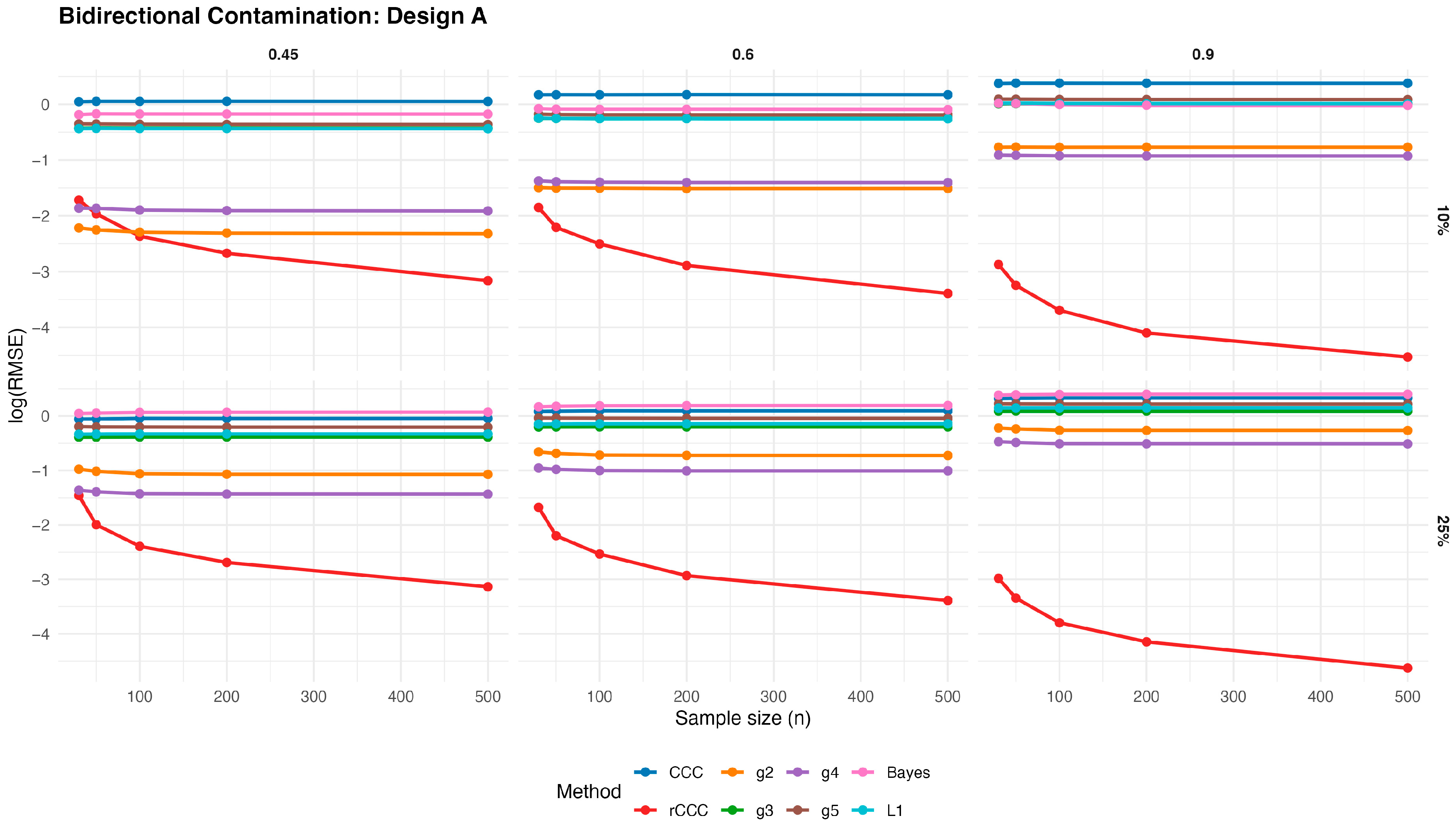
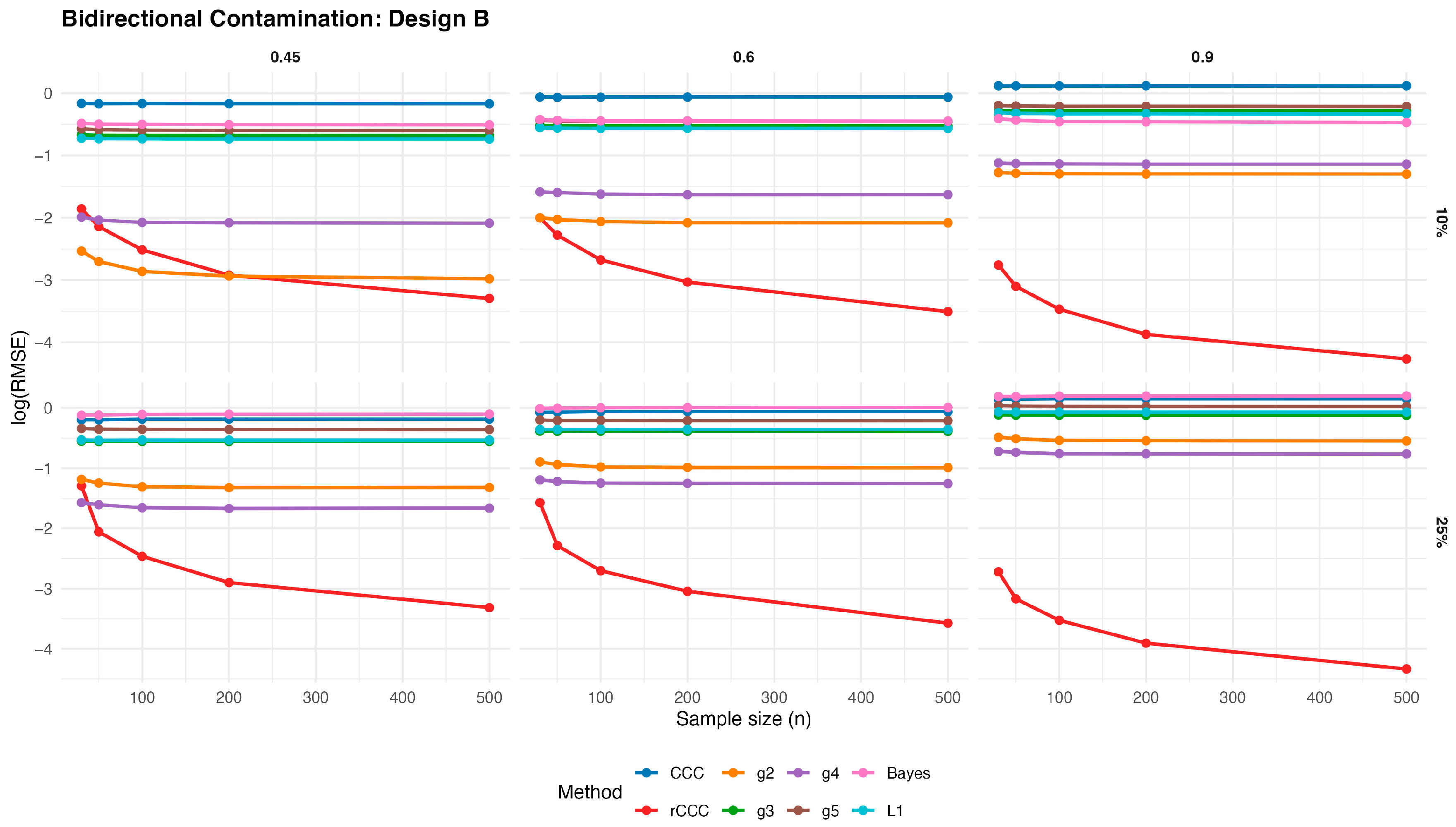
This bidirectional contamination scheme represents a more severe and realistic departure from the ideal model than unidirectional contamination, as entire observations rather than individual variables are affected. Monte Carlo replications are then conducted for each combination of design, sample size, contamination level, and population concordance. 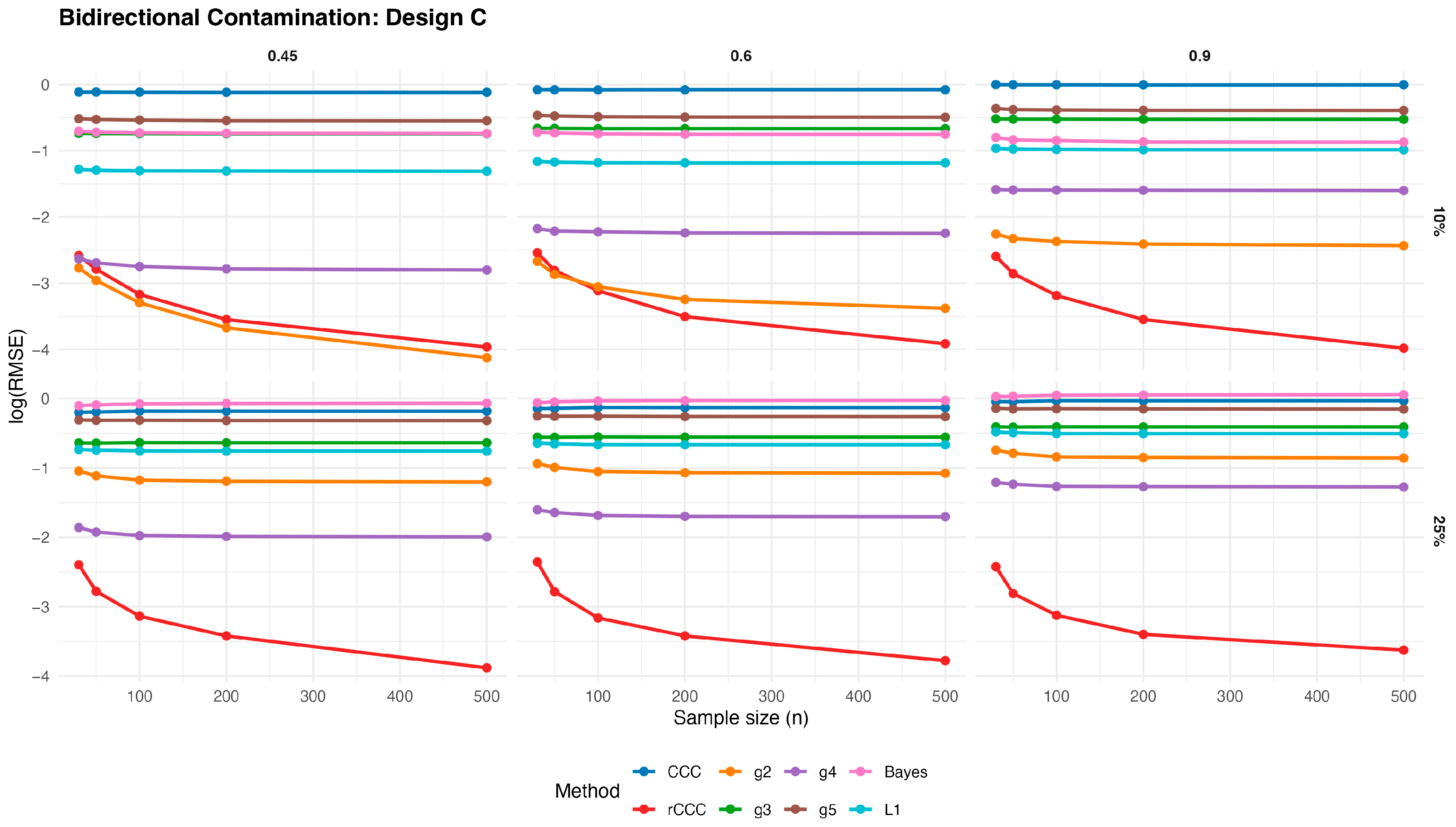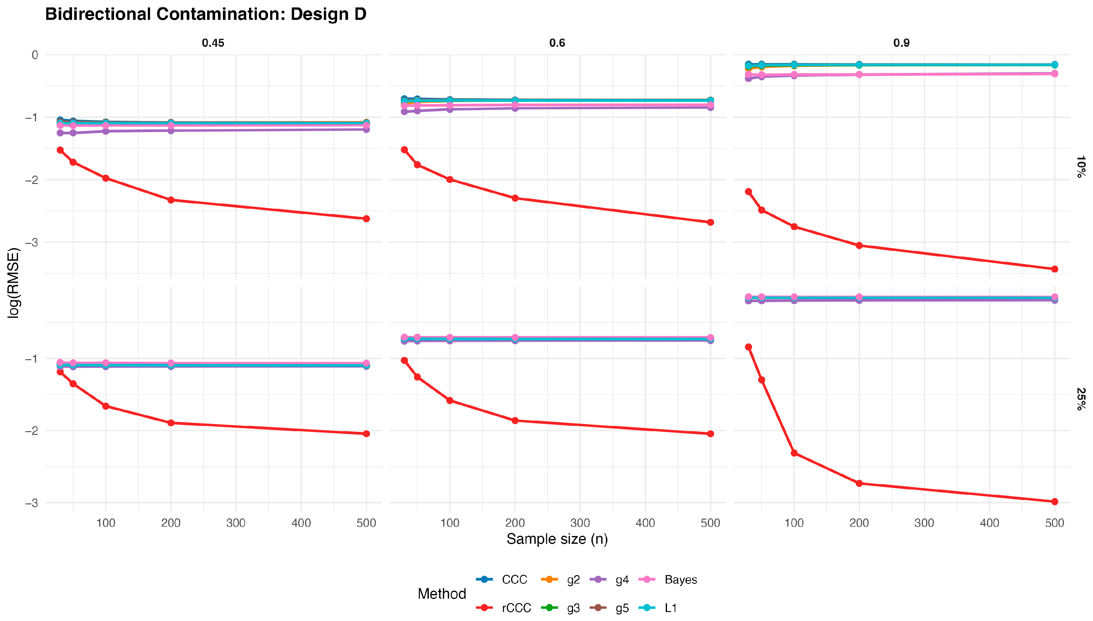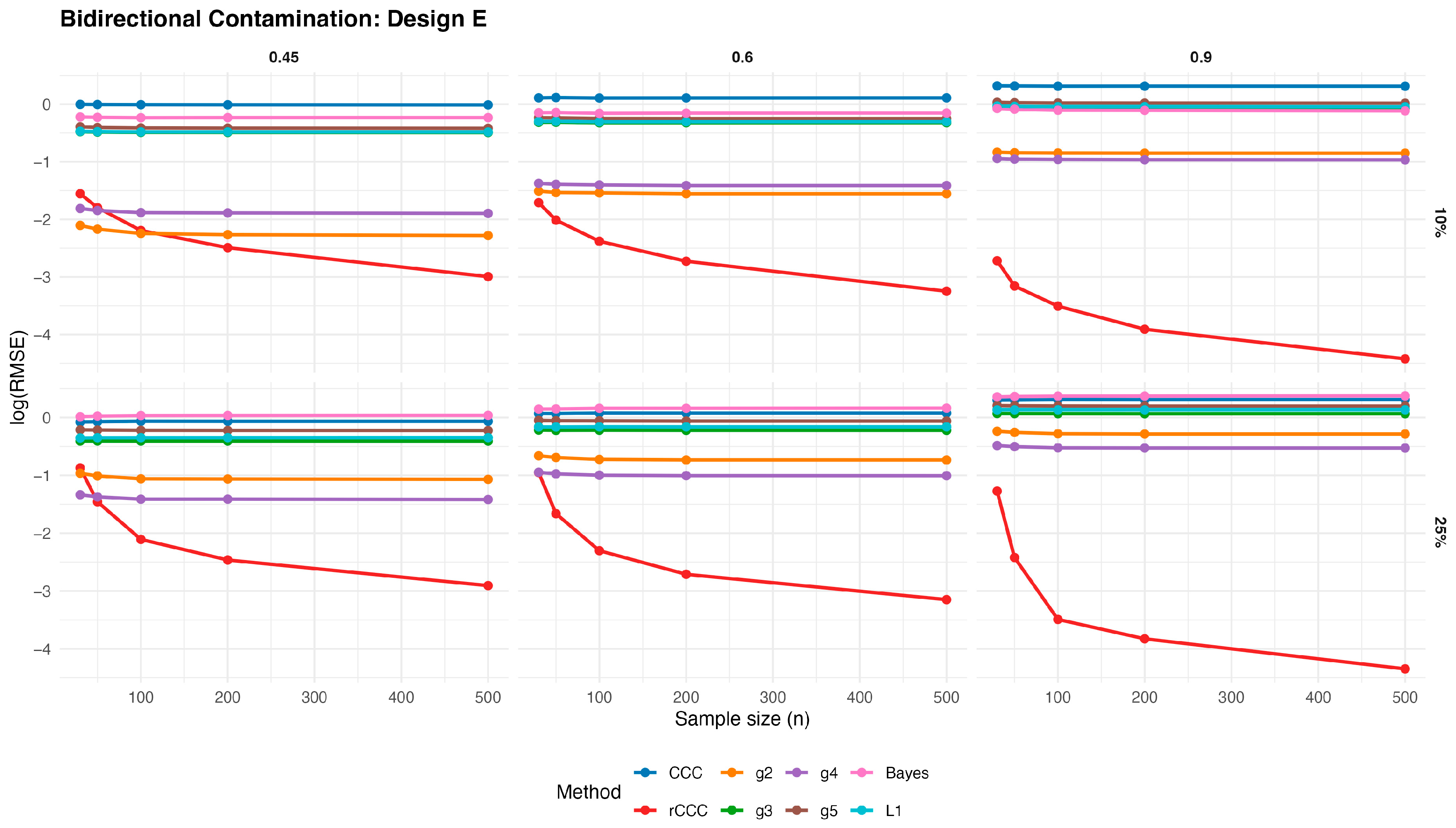The resulting RMSE values are reported in Supplementary File Tables S11–S15, while graphical summaries are presented in Figure 13, Figure 14, Figure 15, Figure 16 and Figure 17.

Figure 13, Figure 14, Figure 15, Figure 16 and Figure 17 present the log(RMSE) values of all estimators under bidirectional contamination, where both variables are simultaneously affected by outliers. The results are shown for two contamination levels $\epsilon =10\%$ and $\epsilon =25\%$ and three population correlation values $\left(0.45, 0.6, 0.9\right)$, across the five designs.

Several clear patterns emerge from these figures. First, in contrast to the clean data case, the classical CCC exhibits a pronounced deterioration under bidirectional contamination. Its error levels remain high and show little improvement with increasing sample size, particularly at moderate contamination levels, highlighting its sensitivity to leverage-type outliers.

Second, the proposed rCCC consistently demonstrates the strongest robustness across all designs, contamination levels, and correlation strengths. In both the 10% and 25% contamination settings, rCCC achieves substantially lower error values than all competing methods, and its $log\left(RMSE\right)$ decreases steadily as the sample size increases. This behavior is especially pronounced at higher correlations $\rho =0.9$, where rCCC clearly separates from the other estimators.

Third, the alternative robust concordance measures based on the g2–g5 functions show mixed performance. While these methods offer some protection against contamination compared to the classical CCC, their error levels remain noticeably higher than those of rCCC, particularly under heavier contamination. Among them, g4 and g5 tend to be more stable than g2 and g3, yet none consistently match the robustness-efficiency balance achieved by rCCC.

Fourth, the L1-based and Bayesian estimators exhibit improved robustness relative to the classical CCC, especially under moderate contamination. However, their performance remains inferior to rCCC across most scenarios. In particular, their error curves often flatten as the sample size increases, indicating limited gains from additional observations under severe contamination.

Finally, increasing the contamination level from 10% to 25% amplifies the differences between the estimators. While the performance of CCC, g-based, L1, and Bayesian methods deteriorates substantially, the proposed rCCC maintains stable and comparatively low error levels. This robustness persists across all five designs, including skewed and heavy-tailed distributions, confirming that the proposed method effectively handles bidirectional and leverage-type contamination.

Overall, the bidirectional contamination results reinforce the advantages of the proposed rCCC. Unlike the clean data case—where rCCC matches the efficiency of CCC—under contaminated settings rCCC clearly outperforms all competing estimators, providing reliable agreement assessment even in the presence of severe and symmetric outliers.

To enhance transparency and reproducibility, we have made a representative sample of the simulation framework publicly available. Specifically, a fully executable example corresponding to Design A, including clean, unidirectional, and bidirectional contamination scenarios, is provided in a public GitHub repository (version 1) [21]. This example illustrates the data generation mechanism, contamination schemes, and performance evaluation based on RMSE with respect to the true population correlation, consistent with the simulation methodology described in this section. The complete large-scale simulation study reported in the paper involves additional designs and extensive repetitions, and is therefore not fully included.

4. Real Example

In order to demonstrate the practical performance of the proposed robust concordance correlation coefficient ${\rho }_R$, we considered two real data applications from different fields: a glucose measurement dataset [22] and a blood pressure dataset [23].

4.1. Glucose Data Example

In this subsection, we use the well-known glucose dataset from the R package MethComp (version 1.30.2) [22]. This dataset contains glucose measurements obtained from serum and plasma samples of the same individuals at different time points. Following the approach of King and Chinchilli [15], we focused on the baseline measurements (time = 0) and compared plasma versus serum readings.

First, we computed the correlation coefficients using the clean dataset, in which the plasma–serum relationship is strongly linear and free of obvious outliers. Subsequently, we introduced an artificial outlier (plasma = 15, serum = 2) to deliberately disrupt the concordance between the two methods. This allowed us to investigate how sensitive each coefficient is to contamination. All results are summarized in the Glucose Data section of

Table 2. Comparison of correlation coefficients under clean and contaminated real data sets.

	Glucose Data		Blood Pressure Data
Coefficient	Clean Data	Contaminated Data	Clean Data	Contaminated Data
${\mathit{\rho }}_{\mathit{P}\mathit{e}\mathit{a}\mathit{r}\mathit{s}\mathit{o}\mathit{n}}$	0.927	−0.458	0.953	−0.81
${\mathit{\rho }}_{\mathit{C}}$	0.897	−0.351	0.947	−0.672
${\mathit{\rho }}_{\mathit{R}}$	0.918	0.918	0.976	0.974
${\mathit{\rho }}_{{\mathit{g}}_2}$	0.685	0.437	0.812	0.267
${\mathit{\rho }}_{{\mathit{g}}_3}$	0.820	0.136	0.906	−0.147
${\mathit{\rho }}_{{\mathit{g}}_4}$	0.502	0.712	0.686	0.524
${\mathit{\rho }}_{{\mathit{g}}_5}$	0.812	0.145	0.905	−0.223
${\mathit{\rho }}_{\mathit{B}\mathit{a}\mathit{y}\mathit{e}\mathit{s}}$	0.827	0.760	0.965	−0.224
${\mathit{\rho }}_{\mathit{L}1}$	0.633	0.259	0.791	−0.193

.

As shown in Table 2, the glucose data example clearly demonstrates the sensitivity of different concordance measures to contamination. While all coefficients indicate strong agreement between plasma and serum measurements under clean conditions, the introduction of a single influential outlier leads to substantial deterioration in several methods. Pearson’s correlation and the classical concordance correlation coefficient collapse to negative values, indicating a complete breakdown of agreement. The robust variants proposed by King and Chinchilli exhibit inconsistent behavior, with some estimators decreasing sharply and others increasing, reflecting instability in the presence of leverage points. The Bayesian CCC and the L1-based CCC show partial robustness: although they remain positive after contamination, both experience noticeable reductions compared to their clean-data values, indicating sensitivity to extreme observations. In contrast, the proposed robust concordance correlation coefficient ${\rho }_R$ remains entirely unchanged under contamination, highlighting its strong resistance to outliers while maintaining efficiency in clean data settings.

4.2. Blood Pressure Data Example

In this subsection, we use the blood pressure dataset (bpres) from the R package cccrm [23], which contains systolic and diastolic blood pressure measurements collected from 384 subjects using two instruments: a manual (mercury sphygmomanometer) device and an automatic device. Each subject was measured twice by each method, yielding replicated paired observations. For comparability with the glucose example, we focus on systolic blood pressure (SIS) and construct one paired value per subject and method by taking the median across replicates, resulting in a clean paired sample (manual vs. automatic) without missing values.

First, we computed the competing concordance measures using the clean paired SIS data, where the agreement between the two instruments is high and no extreme discordant points are evident. Subsequently, to assess robustness, we introduced a deliberately discordant contamination by appending an artificial leverage-type observation designed to disrupt agreement (i.e., one method taking an unusually high systolic value while the other is set to an unusually low value), thereby creating a severe outlier in the method-comparison setting. All results are summarized in the Blood Pressure Data section of Table 2.

As shown in Table 2, the blood pressure example confirms that several coefficients are highly sensitive to a single extreme discordant point: Pearson’s correlation and the classical CCC can flip sign and become strongly negative, indicating that agreement can be misrepresented under contamination. The robust variants of King and Chinchilli again behave inconsistently across contamination, with some remaining positive while others deteriorate substantially or change sign, reflecting method-dependent instability when leverage-type outliers are present. The Bayesian CCC and the L1-based CCC provide only partial protection: both drop markedly and may also change sign under severe contamination, suggesting that they are not fully resistant to extreme discordant observations. In contrast, the proposed robust concordance correlation coefficient ${\rho }_R$ remains essentially unchanged, reinforcing its strong robustness to leverage-type contamination while preserving high agreement in the uncontaminated setting.

These real examples provide strong empirical evidence that ${\rho }_R$ is more reliable than the classical ${\rho }_C$ and other robust alternatives when outliers are present.

5. Software Availability

We have implemented two functions, $ccc\left(\right)$ and $rccc\left(\right)$, in the R package $\mathrm{M}\mathrm{V}\mathrm{T}\mathrm{e}\mathrm{s}\mathrm{t}\mathrm{s}$ [24] to compute the classical concordance correlation coefficient $\left({\rho }_C\right)$ introduced by Lin [1] and the proposed robust concordance correlation coefficient $\left({\rho }_R\right)$. The $ccc\left(\right)$ function requires two arguments, $x$ and $y$, which are numeric vectors containing the observed values of the two variables to be compared. The $rccc\left(\right)$ function extends this by including an additional argument, alpha, which controls the robustness of the Minimum Covariance Determinant (MCD) estimator. Specifically, alpha is a trimming parameter that can take values between 0.5 and 1 (default: alpha = 0.75), reflecting the proportion of uncontaminated data assumed in the analysis. A lower alpha increases robustness against outliers.

With these functions, researchers can easily apply both the classical and robust concordance correlation coefficients to real datasets. The robust version (rccc) is particularly useful when the data are contaminated by outliers, as it yields more reliable estimates of agreement. The MVTests package (version 2.3.1) can be installed directly from GitHub using the following code:

install.packages("devtools")

devtools::install_github("hsnbulut/MVTests")

In addition, all R functions and analysis scripts used to generate the results presented in this paper, including the real-data applications, are publicly available in a dedicated GitHub repository at: https://github.com/hsnbulut/rccc (accessed on 30 December 2025).

6. Conclusions

This paper introduced the robust concordance correlation coefficient (rCCC), which replaces the classical mean, variance, and covariance estimators in the CCC formula with robust alternatives derived from the Minimum Covariance Determinant (MCD). The proposed approach directly addresses the well-documented sensitivity of the classical CCC to outliers and skewed distributions.

The findings from an extensive Monte Carlo simulation study across five different designs provide compelling evidence of the advantages of rCCC. In clean data scenarios, rCCC behaves almost identically to the classical CCC, showing that the introduction of robustness does not cause efficiency loss. In contaminated scenarios with 10% and 25% outliers, rCCC consistently achieved the lowest RMSE values among all competitors, including the classical CCC and the King–Chinchilli’s robust variants. This stability was observed across varying sample sizes, correlation levels, and distributional forms, confirming the general applicability of the proposed method.

The observed variability in the performance of the King–Chinchilli variants across different simulation settings can be attributed to their reliance on moment-based components and weighting schemes. In particular, these approaches combine measures of precision and accuracy through variance- and covariance-driven adjustments, which may become unstable under contamination or distributional asymmetry. As a result, small changes in variance structure or the presence of outliers can disproportionately influence the estimated concordance, leading to performance that is highly scenario-dependent.

The real data example using plasma and serum glucose measurements offered further support. When a single artificial outlier was introduced, both Pearson’s correlation and the classical CCC collapsed, even yielding negative estimates of agreement. In contrast, rCCC remained virtually unchanged, providing a realistic and reliable measure of concordance.

Beyond its theoretical and empirical contributions, the practical relevance of rCCC has been enhanced by its implementation in the R package MVTests. Researchers can now easily compute both classical and robust CCCs using simple functions, with the trimming parameter α offering additional control over robustness.

Taken together, this study demonstrates that rCCC is both a robust and efficient estimator. It provides reliable results under clean data and substantial protection against outliers under contaminated data. Therefore, rCCC should be considered a strong alternative to the classical CCC in biomedical, clinical, and other applied research settings where measurement agreement is of critical importance.

Potential directions for future research include extending the proposed robust concordance correlation coefficient to repeated measures and longitudinal settings, where within-subject dependence must be explicitly accounted for. Another promising avenue is the development of multivariate or high-dimensional versions of the robust CCC, enabling agreement assessment among more than two measurement methods. Such extensions would further broaden the applicability of the proposed approach in complex real-world data structures.