Abstract
Dual-channel retailing empowers the manufacturer to benefit from market opportunities by producing customized items that fulfill client requirements. The manufacturer and retailer sell customized products, which allow customers to express their chosen style to increase both the likelihood of customers making a purchase and their level of satisfaction with the product. This trend is demonstrated by the current study, in which customized consumer items are considered through online and offline channels. On the other hand, cybersecurity has become a crucial aspect of the digital era, ensuring the protection of sensitive data, networks, and systems from cyberattacks and unauthorized access. This study develops with a modern cybersecurity framework to protect against cyberattacks and increase customer trust. This model is based on customized product design, cybersecurity investment, advertisement investment, and increasing the green level of customized products. The model is solved using both centralized policy and vertical Nash policy. Numerical results indicate that centralized profit is 2.37% more than the decentralized profit. Without investing in customized products and cybersecurity, the profit of the supply chain decreases by 2.33% and 1.99% for the centralized method, 1.28% and 1.15% for the vertical Nash method for the retailer, and 1.85% and 1.38% for the vertical Nash method for the manufacturer.
MSC:
90B05; 90B06
1. Introduction
In today’s market, the customized product business is a popular trend [1]. This is because consumer taste in products is constantly evolving. Therefore, the demand for customized products has been steadily growing worldwide. Using customized products, the consumer can express their needs through their style to satisfy their expectations. The consumer places an order for a product according to their preferences, and the manufacturer then makes the product following those desires. When this occurs, the store can earn a profit, since the customer finally receives the products they desire, is satisfied with their purchase, and is willing to pay the cost of the customized product. The firm offers customized items to satisfy the desire of the customer and run the business successfully and efficiently [2]. The retail channel promotes its brand by sharing its customized products online [3]. Implementing a successful plan enables members of the supply chain to enhance their sales volume and market share. In particular, retail channels are primarily concerned with boosting the number of transactions, which can be boosted by environmentally green products, advertising, and customized products through a dual-channel strategy. Manufacturers and retailers employ several technologies to adapt customer behavior.
With the growing customized product industry and increasing use of technology, cybersecurity is a problem that is receiving attention and significance on a global scale [4]. The most prominent problem that various firms are dealing with is cyberattacks [5]. Multiple threats, including malware, spam, phishing attacks, and distributed denial-of-service attacks can produce cyberattacks. Several organizations are required to prioritize protecting themselves from unfamiliar attacks. Hence, it is necessary for every organization to consider the dangers to which they are frequently exposed and to carry out their operations in such a manner that they can minimize the vulnerabilities to the greatest possible extent. Every year, there has been an increase in the number of cyber breaches that have been reported. Many cyberattacks have been observed recently, and most attacks occur in networking and internet technology. For example, when a famous Bluetooth headphone company creates a design with wireless data transmission, they increase their exposure to cybersecurity threats in the form of unauthorized access, data breaches, and malware infection. Therefore, it is the responsibility of manufacturers to provide secure connections between devices and headphones. A Bluetooth headphone firm will have to possess strong encryption mechanisms, authentication techniques, and periodic firmware updates to safeguard customers’ privacy and build trust.
1.1. Aims and Objectives
The main objective of this study is to provide cybersecurity to supply chain members within a supply chain network (SCN).
- As e-commerce and digital platforms are expanding exponentially, retailers are faced with disastrous issues in data protection and customer trust; hence, it is imperative to create effective cybersecurity strategies. At the same time, customers want more personalized experiences, and businesses are challenged to create customized products with their own individual priorities in focus, resulting in increased customer satisfaction and loyalty.
- This study is driven by the pressing global imperative for eco-friendly business practices; the challenge is the integration of green innovation in production and distribution to ensure environmental and economic gains. Effective advertising strategies also play a crucial role in influencing the minds of consumers and conveying the value of customized and sustainable products. Finally, dual-channel retailing helps all types of customers buy products according to their own priorities and put businesses ahead in the competitive market.
- By combining these dimensions, this study aspires to advance theory and offer managerial suggestions for creating a secure, sustainable, and customer-oriented retail atmosphere in order to survive and thrive in the green and digital economy.
1.2. Research Questions
Some research questions of this study are discussed below.
- What will be the profit of the retailer, manufacturer, and supply chain if it has cybersecurity issues for online and offline channel? Can the proposed policy provide more profit than either the online cybersecurity issue or offline cybersecurity issue alone?
- In the face of green innovation and advertisement issues, will the customized product dual-channel strategy be beneficial for both the player and the supply chain?
- What is the best dual-channel retailing strategy for maximizing the profit using green innovation, advertisement, cybersecurity, and customized products?
1.3. Contribution of This Study
To address the above research gaps, this study proffers the following contributions (Figure 1).
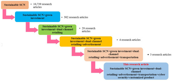
Figure 1.
Research work on cybersecurity and customized products (data source: https://www.sciencedirect.com/; 1 August 2025).
- To run businesses efficiently and smoothly in today’s competitive and globalized market, supply chain members provide the service of customized products based on customer preferences to give customer satisfaction through online and offline channels.
- To develop brand trust and avoid interrupted operations, supply chain members invest in strong security measures, which ensure that the customer can collaborate easily and happily in the near future.
- To develop environmental growth, the manufacturer makes green products. The manufacturer and retailer transport products using railway transportation, which is more eco-friendly than other transportation systems.
- To increase sales and enhance brand reputation, advertising services are provided by supply chain members.
1.4. Orientation
The remainder of this study has been partitioned into the following sections. The relevant literature is discussed in Section 2. In Section 3, notation, assumptions, and the problem definitions are discussed. The mathematical model is explained in Section 4. Section 5 shows the solution methodology. In Section 6, numerical analysis and discussions are explained, and managerial insights are discussed in Section 7. Finally, conclusions and future extensions of this study are elaborated in Section 8.
2. Literature Review
This study focuses on online and offline customized products and cybersecurity in the green supply chain. The related literature is studied and discussed in this section. A comparative review is given in a tabular form in Table 1.

Table 1.
Authors’ contributions.
2.1. Influence of Customized Product Under Dual-Channel Channel
In the competitive market, supply chain members use various policies and strategies to maintain a stable demand in the market [20]. Manufacturers and retailers open dual-channel retailing to provide better service to customers. For example, as customers follow trends in fashion, they try to distinguish themselves and their style from others. To meet the demands of this fashion trend, supply chain members have begun to make customized products. Huang et al. [21] proposed a two-stage customized packaging strategy designed to maximize profit, addressing consumer demands to improve consumer loyalty and happiness. However, this study avoided explaining the advantages of cybersecurity. Flacandji et al. [22] demonstrated a retail application that does not enhance consumers’ perception of independence but does enhance their sense of ability. Wang et al. [23] presented a closed-loop supply chain (CLSC) model where they focused on product customization under dual-channel retailing. According to them, the manufacturer marketed customized products via online channels only, but the manufacturer marketed regular products through both online and offline channels.
Manufacturer decision-making based on opening a live-streaming shopping channel was examined by Zhang and Tang [24]. They showed that it is possible for manufacturers to earn more profit by opening a live-streaming shopping channel but ignored discussion on the advantages of advertisement. Kim et al. [25] examined small-sized stores and assessed whether such a store should use a dual-channel retailing strategy or not that in the competitive market. They proved that dual-channel retailing is always an advantageous idea for small-sized stores. Pan et al. [26] developed a novel approach for designing customized products. The study focused on a re-commendatory configuration design method for customized products and showed that profit increases 99.51% when using that approach. However, the study did not discuss cybersecurity and advertising. Hosseini-Motlagh et al. [27] demonstrated competition between two types of retailers—an electronic retailer and a traditional retailer using dual-channel retail—where a warranty replacement policy is offered by the electronic retailer, whereas the traditional retailer offers sales services to customers. However, the study did not consider the benefits of advertisement.
2.2. Impact of Advertisement and Selling Price Driven Demand in Supply Chain
Supply chain members impose many strategies by adjusting demand balance in the market to earn more profit for the SCN. Demand may not be constant at all times; as such, the selling price is an important decision in achieving higher demand. A lower selling price is always beneficial for earning more profit in the competitive market. Lu et al. [28] investigated the effect of users viewing advertisement videos in the business sector. This study focused on comparing user ratings for the effectiveness of advertisement videos. Mirzagoltabar et al. [29] designed an SCN in the lighting industry, where the price of dual-channel retailing and demand are considered as uncertain. The study investigated customer behavior in relation to the selling price of the product. However, the study avoided discussing the benefits of customized products and cybersecurity. To provide an electronic shopping experience to customers, Zhang et al. [30] presented a supply chain management (SCM) model, where the manufacturer offers three different electronic channels and showed competition between channels. A price competition between two retailers (a traditional retailer and an e-retailer), was designed by Qiu et al. [31] in a supply chain model considering dual-channel retail. They assigned the manufacturer as a leader and both retailers as followers. Along with the selling price, advertising takes a big role in earning more profit in a supply chain network. When a retailer advertises a product with all its features and necessities, then customers know about the product and become interested in buying the product. However, this study did not consider green innovation, customized products, and cybersecurity in their study.
Nishio and Hoshino [32] published a study demonstrating the necessity of integrating advertising rewards into a corporate loyalty program. Competition between the manufacturer and retailer was considered by Pei and Yan [33], where the manufacturer advertises products to customers through online retailing. Sarkar et al. [34] worked on a biodiesel-based supply chain. The study discussed the risk of biodiesel production in the supply chain network. However, they avoided discussing cybersecurity and a customized products. Gao et al. [35] presented a CLSC network where the demand is uncertain in the dual-channel retailing for the appliance industry. The study focused on advertisement but avoided discussion on green products, customer security, and customized products. Kumar et al. [36] examined retail price strategy. The study proposed a smart approach to payment policy. They focused on using advertisement and selling prices to obtain an advantage in the competitive market but not on the effect of customized products and cybersecurity. Chaudhari et al. [37] studied advertisement, price, and stock depending on demand. They introduced how advertisement, the down-cash-credit method, deteriorating product, and carbon tax regulation impact business strategies. Motlagh and Nasiri [38] developed a model to optimize pricing strategies in a dual-channel retailing under an SCM with incorporates a discount policy. They incorporated a revenue-sharing contract between supply chain members, and the demand is dependent on price and uncertainty to earn more profit.
2.3. Effects of Cybersecurity in Supply Chain
Recent advancements in communication and web technology have led to an increase in cyberattacks across all industries. Incidents involving ransomware have become one of the most critical cybersecurity risks confronting organizations globally. In recent years, ransomware has increasingly targeted vital facilities and cyber–physical systems (CPS), including industrial control systems and healthcare networks [39]. Patient empowerment and digital health records have become essential in the evolving landscape of healthcare delivery, as patients increasingly adopt a proactive role in managing their health, as was introduced by Govindarajan et al. [40]. This study did not use green innovation. Jana and Ghosh [41] developed and refined a comprehensive risk assessment framework for cybersecurity. Their methodology aimed to improve the ability to predict risks related to cybersecurity despite uncertainties in data and information stemming from various criminal activities. Li et al. [42] worked on cybersecurity in the supply chain. This study focused on securing customers for buying online products in the business sector by providing cybersecurity. However, the study did not discuss the benefits of customized products. Wang [43] introduced analytical models to optimize corporate cybersecurity expenditures and cyber insurance, focusing on the efficacy of investments in mitigating cyberattacks, vulnerabilities, and consequences. The study focused on customer reactions to cyber threats. Gombár et al. [44] discussed cybersecurity risks in industry. The study proposed a framework of hybrid threads based on risk perception analysis. Tayyab et al. [45] experimented with the utilization of serial production technology that helped to develop a production model. But they did not discuss security technology that could help the serial production system for information security.
2.4. Transportation in Supply Chain
Transportation is very important in any industry. All industries want to reduce transportation costs to stay ahead in business. Rajabion et al. [46] introduced the influence of urban transportation on agricultural products. The study explained many types of competitive advantages for agricultural product distribution in the urban area. Samanta et al. [47] developed a transportation strategy for smart production. The study showed how transportation affects the human society in the complex retail sector. Saen et al. [48] investigated the effectiveness of non-convex double frontiers in the context of sustainable transportation supply chains. This study presented a new and innovative nonconvex double frontier method, known as the network-free disposal hull, for assessing sustainable supply chains. Sherif et al. [49] worked on inventory, transportation, and vehicle routing in a green supply chain network. The study introduced environmental regulations and economic concerns for the battery industry. Nugroho and Zhu [50] explained a transportation planning approach for syngas and hydrogen in the supply chain. The study proposed a strategic transportation and supply planning model with the objective of maximizing supply chain profit in consideration of supply capacity, available biomass, and transportation cost. However, the study avoided explaining green innovation and dual-channel retailing. Tayyab et al. [51] investigated fuzzy programming approach with a sustainable SCM. It demonstrated how a supplier can minimize transportation costs and provide maximum profit. Yige et al. [52] investigated government subsidies for transportation in the supply chain. The study introduced the effect of shipping enterprises on green transformation for social responsibility.
2.5. Effect of Green Innovation Within Supply Chain
The latest literature observes that green innovation is an enhancer of operational efficiency, competitiveness, and sustainability in the long-range sense for supply chain management. Debnath and Sarkar [53] worked on circular economy for achieving sustainable development. The study focused on reuse of materials and waste reduction but did not explain the benefit of green innovation and cybersecurity. Alamri et al. [54] discussed a sustainable inventory model for an imperfect item. They focused on preservation techniques to obtain a long-lasting product, advertising to attract customers, reducing carbon emissions to reduce greenhouse gas, and waste management for maximum profit. Habib et al. [55] developed a flexible programming approach in the supply chain. The study investigated the risk and benefit of fossil fuels. Ahmed et al. [56] focused on reworking an imperfect product in the supply chain, providing repair of defective products in the local market to maximize overall profit. Yadav et al. [57] examined the environmental effect of bi-product management but without the usage of cybersecurity. Levi-Bliech and Dahan [58] discussed the influence of green items in the green supply. The study showed that the supply chain and green innovation enhance the social performance of an organization. However, they did not introduce a customized product. Guchhait and Sarkar [59] developed a decision-making strategy in the global supply chain. The model introduced a multi-retailer and manufacturer model, which explained environmental, economic, outsourcing, and service issues.
3. Problem Definition, Notation, and Assumptions
The problem’s definition, notation, and assumptions are discussed here.
3.1. Problem Definition
An SCN model is observed with one manufacturer and one retailer. The manufacturer sells products through an online channel to the customer at the wholesale price and through an offline channel to the retailer. The retailer sells those products to customers through an offline channel. The manufacturer offers a fixed discount to the retailer due to the large volume ordered by the retailer. Both the retailer and manufacturer invest capital for cybersecurity, greenness, and customized product design. Additionally, the retailer invests in advertisement. The model is solved by vertical Nash (VN) and centralized policy (CP) methods. The framework of the model is depicted in Figure 2.
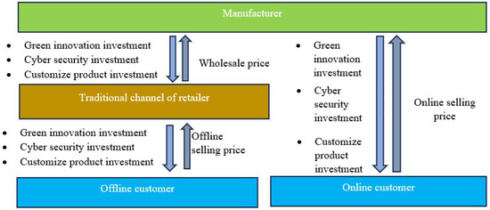
Figure 2.
Problem description of the study.
3.2. Notation
All notation of this study are given in Table 2.
Table 2.
Notation.
3.3. Assumptions
The assumptions of the research problem are as follows:
Assumption 1.
An SCN model consists of one manufacturer and one retailer, where the manufacturer produces customized products and sells directly to the customer through an online channel and to retailer through an offline channel. After receiving products, the retailer sells products to the customer through an offline retail channel.
Assumption 2.
The market demand of the customized product is non-linear. The market demand depends upon the selling price of online and offline channels, advertisement, cybersecurity, customized product design, and the greenness of the product. The offline demand is , and the online demand is .
Assumption 3.
The retailer invests in advertisement for increasing customer trust, sales, and brand value, where ν is the cost coefficient of advertisement and ς is the level of advertisement. The manufacturer invests in green innovation ϰ.
Assumption 4.
The retailer invests in cybersecurity. The manufacture invests and in cybersecurity through online and offline channels, respectively, where , , and are the respective investment coefficients.
Assumption 5.
The retailer invests in customized products. The manufacture invests and in customized product through online and offline channels, respectively, where , , and are the respective investment coefficients.
Assumption 6.
The manufacturer provides a fixed discount on the online selling price to the retailer due to the large quantity ordered by the retailer. This means that the retailer purchases items from the manufacturer at the wholesale price , which is decided by the manufacturer, where is the online selling price.
Assumption 7.
The manufacture and retailer use railway transportation for shipments. The fixed and variable transportation cost of the manufacturer are and , respectively. The fixed and variable transportation costs of the retailer are and , respectively.
4. Mathematical Model Formulation
One manufacturer and one retailer engage in the SCN. The offline market demand of the customized product is
and the online market demand is
where a is base market demand, is the customer’s choice of preferred channel, is a scaling parameter for demand for the associated channel, is the offline selling price, is a scaling parameter associated with demand for the opponent’s channel, is the online price, c is a scaling parameter related to a product’s greenness, is the level of greenness, is the scaling parameter related to advertisement, is the level of advertisement, is a scaling parameter for cybersecurity of the manufacturer through the offline channel, is manufacturer’s offline cybersecurity, is the shape parameter for the cybersecurity of the manufacturer through the offline channel, is a scaling parameter for cybersecurity of the retailer through the offline channel, is the retailer’s offline cybersecurity, is the shape parameter for the cybersecurity of the retailer through the offline channel, is a scaling parameter for customized products of the manufacturer through the offline channel, is the manufacturer’s offline customized product, is the shape parameter for the manufacturer’s customized product through the offline channel, is a scaling parameter for the customized product of the retailer through the offline channel, is the retailer’s offline customized product, is the shape parameter for the customized product of the retailer through the offline channel, is the scaling parameter for manufacturer cybersecurity through the online channel, is the manufacturer’s online cybersecurity, is the shape parameter for the cybersecurity of the manufacturer through the online channel, is a scaling parameter for the manufacturer’s customized product through the online channel, is the manufacturer’s online customized product, is the shape parameter for the product customized by the manufacturer through the online channel.
Costs, revenues, and profits of the manufacturer and retailer within the SCN are discussed below.
4.1. Manufacturer’s Model
The manufacturer sells customized products to customers at a wholesale price online, and the retailer sells offline. The manufacturer uses railway transportation to transport products. The total demand of the manufacturer is . There are three types of investment by the manufacturer: green investment, cybersecurity investment, and customized product design investment. The different costs of the manufacturer are discussed below.
4.1.1. Revenue
The manufacturer sells products to customers through an online channel at ($/item) and to the retailer through an offline channel at a wholesale price . The wholesale price comes with a fixed discount h on the online selling price . Then, the wholesale price becomes ($/item). and are the offline and online demand, respectively. Hence, the total revenue of the manufacturer is as follows:
4.1.2. Cybersecurity Investment
To secure the digital asset from cyberattacks and associated risks, the manufacturer uses some precaution. The cybersecurity precautionary measure is used in both channels. and represent cybersecurity investment for the online and offline channels, respectively. and represent the associated cybersecurity usage. Hence, the manufacturer’s investment for cybersecurity for both channels is as follows:
4.1.3. Customized Product Design Investment
The manufacturer receives an order for customized products from market. Hence, after production of a base product, the manufacturer customizes products based on the demand. For online and offline channels, the manufacturer invests in customized product production facilities. and are the customized product investment parameters. and are the associated customized product design for the online and offline channels, respectively. Therefore, the total investment for customized product design is as follows:
4.1.4. Green Innovation Investment
The customized product is an eco-friendly product and has a green innovation level. The manufacturer maintains green innovation for the customized products. is the green investment, and is the green innovation level. Hence, the manufacturer’s green innovation investment is as follows:
4.1.5. Transportation Cost
The manufacturer uses transports for raw materials. The manufacturer invests and for variable and fixed transportation purposes, respectively. Hence, the total transportation cost of the manufacturer is
4.1.6. Total Profit of the Manufacturer
4.2. Retailer’s Model
The retailer sells the customized products through an offline channel. The demand of the retail channel is . The revenue and costs of the retailer are discussed below.
4.2.1. Revenue from Selling
The retailer generates revenue from the offline channel by selling products on the market. The retail price of product is . The total revenue of the retailer is given bellow.
4.2.2. Advertisement Investment
The retailer uses advertisement to obtain more customers than they would otherwise. An additional investment is required in that case. The investment scaling parameter of the advertisement is , and the advertisement level is . Hence, the advertisement investment is explained in Equation (10).
4.2.3. Purchasing Cost
The retailer’s demand is and the retailer buys product from the manufacturer at a rate , where h is the fixed discount and is the online selling price. Hence, the purchasing cost of the retailer is
4.2.4. Transportation Cost
The retailer uses rail transport for carrying product from the manufacturer’s store to the retail store. The retailer has the unit transportation costs and for variable and fixed transportation, respectively. Hence, the total transportation cost of the retailer is shown in Equation (12).
4.2.5. Cybersecurity Investment
The retailer invests in cybersecurity for protection from digital risks. The investment scaling parameter for the cybersecurity of the retailer is , and the cybersecurity level of the retailer is . The cybersecurity investment is explained in Equation (13).
4.2.6. Customize Product Design Investment
The retailer contributes to the customized product design alongside the manufacturer. Thus, the retailer invests in customized product design. The investment scaling parameter of the customized product design of the retailer is and the customized product design level of the retailer is . The customized product investment is explained in Equation (14).
4.2.7. Total Profit of the Retailer
4.3. Total Profit of the SCN
5. Solution Methodology
The models are solved using both a CP and decentralized policy based on a VN game. The optimum values of the decision variables in two cases are derived analytically using the classical optimization technique. A brief summary of the above methods is given below:
A CP method coordinates with just one authority for deciding selling prices, advertisement, green innovation, cybersecurity, and customized products. Such an approach diminishes channel conflict, ensures uniform standards, and enhances communication across departments. Managers exercise control over resource allocation, thereby ensuring cost efficiency with greater system profitability. Additionally, the CP method institutionalizes uniform rules and procedures throughout the organization for purposes of risk management. Hence, overall efficiency and strategic alignment in the future are achieved through the centralization of systems, thereby viewing the entire system as one whole integrated body.
A VN method allows each supply chain member to make independent decisions that maximize their own profit, leading to more realistic and practical outcomes in competitive environments. Thus, such a condition leads to a more reasonable and practical representation in competitive environments. The decentralization presents itself as productive market behavior since it operates in the framework of conflicting objectives, constraints, and information sets of manufacturers and retailers. As each party can react significantly faster to changes in the market without waiting for centralized approval, it encourages flexibility and local innovations. Transparency within the VN method is aided by the clear declaration of the optimal strategies and profit contribution of each channel member. Overall, it informs managerial decision-making with respect to how self-interested behavior impacts pricing, production, investment, and coordination within the supply chain.
5.1. CP Method
In this method, the manufacturer and retailer jointly decide the optimum value of the decision variables and try to obtain maximum profit in the system. For finding the optimal results, the first-order partial derivatives of Equation (16) with respect to all decision variable is calculated and set such that they are equal to zero; these are , , , , , , , , , and .
All values of the first-order derivative are given in Appendix B. Please check Appendix B for explicit values. After that, the optimum values of the decision variables are found as follows:
Theorem 1 establishes that Equation (16) has the global maximum value at the above unique solutions. Algorithm 1 is used to find the numerical values in CP method.
Theorem 1.
The objective function in Equation (16) achieves a global maximum at a unique point if the principal minors of its Hessian matrix of order have an alternating sign at the optimal values of the decision variables. That is, the values of the principal minors of the Hessian matrix are , , , , , , , , , and .
Proof.
See Appendix B. □
| Algorithm 1: Algorithm to find the global numerical solution in CP method | |
| Step 1. | Give all parameter’s values and set the loop counter i. |
| Step 2. | Set the initial values of parameters. |
| Step 3. | Evaluate from Equation (17) utilizing the values of Step 2. |
| Step 4. | Evaluate from Equation (18) utilizing the values of Step 3. |
| Step 5. | Evaluate from Equation (19) utilizing the values of Step 4. |
| Step 6. | Evaluate from Equation (20) utilizing the values of Step 5. |
| Step 7. | Evaluate from Equation (21) utilizing the values of Step 6. |
| Step 8. | Evaluate from Equation (22) utilizing the values of Step 7. |
| Step 9. | Evaluate from Equation (23) utilizing the values of Step 8. |
| Step 10. | Evaluate from Equation (24) utilizing the values of Step 9. |
| Step 11. | Evaluate from Equation (25) utilizing the values of Step 10. |
| Step 12. | Evaluate from Equation (26) utilizing the values of Step 11. |
| Step 13. | Set all the above-proposed steps utilizing the amended values of , , , , , , , , , and . Until the values of , , , , , , , , , and from and i become the same, repeat Steps 3 to 12. |
| Step 14. | Calculate the total profit of SCN by substituting the values of , , , , , , , , , and into Equation (16). This is the maximum profit, and , , , , , , , , , and are the optimal solutions. |
| Step 15. | Stop. |
5.2. VN Method
For the decentralized case, the optimum solutions are obtained using vertical Nash game. The VN game appears between two different level of supply chain players; in this case, these are the manufacture and the retailer. In this method, both the members take decisions independently. This means that the manufacturer and the retailer both decide the optimum values of their individual decision variables. , , , and are the decision variables of the retailer and , , , , , and are the decisions variable of the manufacturer.
For determination of the optimal result, one can partially differentiate the profit function of the retailer in Equation (15) and the manufacturer in Equation (8) with respect to the corresponding decision variables and set them to be equal to zero; these values are as follows: , , , , , , , , , and . All values of the first-order derivative are given in Appendix C.1 and Appendix C.2. Please check Appendix C.1 and Appendix C.2 for explicit values. The sufficient conditions for the classical optimization establish the global maximum profit at the obtained values. For the manufacturer, the optimum values of the decision variables are
The following Theorem 2 establishes that the obtained profit of Equation (8) of the manufacturer using the above unique solutions are global maximum. For establishing the global maximum, Theorem 2 follows Propositions 1 and 2. Algorithm 2 is used to find the numerical results of the manufacturer in VN method.
Theorem 2.
The global maximum is achieved for Equation (8) if the principal minors of the Hessian matrix of order have an alternating sign. That is, the values of the principal minors of the Hessian matrix are , , , , , and .
Proof.
See Appendix C.1. □
Proposition 1.
, i.e., .
Proposition 2.
, i.e., .
| Algorithm 2: Algorithm to find the global solution for the manufacturer in VN method | |
| Step 1. | Give all parameter’s values and set the loop counter. |
| Step 2. | Set the initial value = 1, = 0.2, = 0.2, = 0.2, = 0.6, and = 0.6. |
| Step 3. | Evaluate from Equation (27),utilizing the values of Step 2. |
| Step 4. | Evaluate from Equation (28),utilizing the values of Step 3. |
| Step 5. | Evaluate from Equation (29),utilizing the values of Step 4. |
| Step 6. | Evaluate from Equation (30),utilizing the values of Step 5. |
| Step 7. | Evaluate from Equation (31),utilizing the values of Step 6. |
| Step 8. | Evaluate from Equation (32),utilizing the values of Step 7. |
| Step 9. | Set the all above-proposed steps utilizing the amended values of , , , , , and . Repeat this method until the values of , , , , , and stay unchanged. |
| Step 10. | Calculate the total profit of the manufacturer by putting the values of , , , , , and , into the Equation (15). This is the optimal profit and , , , , , and , are the optimal solution. |
| Step 11. | Stop. |
The global maximum profit of the retailer in Equation (15) is established by Theorem 3 supported by Propositions 3 and 4. Algorithm 3 is used to find the numerical solutions of Equation (15) in VN method.
Theorem 3.
The global maximum is achieved for Equation (15) if the principal minors of the Hessian matrix of order have an alternating sign. That is, the decision variables , ς, , and for the retailer and the principal minors , , , and have alternating signs.
Proof.
See Appendix C.2. □
Proposition 3.
, i.e., .
Proposition 4.
, i.e., .
| Algorithm 3: Algorithm to find the global solution for the retailer in VN method | |
| Step 1. | Give all parameter’s values and set the loop counter. |
| Step 2. | Set the initial value = 1, = 0.2, = 0.5, and = 0.5. |
| Step 3. | Evaluate from Equation (33),utilizing the values of Step 2. |
| Step 4. | Evaluate from Equation (34),utilizing the values of Step 3. |
| Step 5. | Evaluate from Equation (35),utilizing the values of Step 4. |
| Step 6. | Evaluate from Equation (36),utilizing the values of Step 5. |
| Step 7. | Set all the above-proposed steps utilizing the amended values of , , , and . Repeat this method until the values of , , , and stay unchanged. |
| Step 8. | Calculate the total profit of the retailer by substituting the values of , , , and into Equation (8). This is the optimal profit, and , , , and represent the optimal solution. |
| Step 9. | Stop. |
5.3. Comparison Between CP and VN Methods
Comparing the VN method with the CP method enhances an understanding of how these decision-making structures can affect the supply chain’s performance. The VN method, therefore, captures a close approximation of some real-life situations wherein the manufacturer and the retailer act independently and optimize their own profits in light of issues such as channel conflict, inefficiency, and competition. On the opposite end, the CP method examines an ideal coordinated scenario whereby decisions are jointly maximizing for the total profit of the system. Thus, a strong push for comparison will be provided to starkly indicate the effect of cooperation versus self-interest, the performance gaps that arise, and ways to bridge these gaps for better coordination and hence supply chain efficiency. Through a comparative study, it is found that the CP method is best for this study.
6. Numerical Analysis
To validate the model numerically, the following numerical experiment has been performed, and the input values of parameters are taken from the literature [60] at their best fit. The input parameters are as follows: ; ; units; ; ; ; ; ; ; ; ; ; ; ; ; /unit; ; /unit; ; ; ; ; ; ; ; ; ; ; ; ; . For the VN method in retailer’s case, = 3.603 and = 3.665. For the manufacturer’s case in the VN method, = 119.33 ($/unit), = 2.35, = 2.32, and = 2.30.
The optimal results are obtained using those parametric values in Matlab R2025a. The computational time to obtain the results in MATLAB 12 was less than 5 s. In this result, the tolerance is zero because for the iteration, the value of the step and step are the same for some positive integer p, where . The optimum values of the decision variables and the total profit are given in Table 3. The highest profit is obtained with the CP method followed by the VN method. A graph showing concavity in response to different decision variables across several scenarios is shown in Figure 3.
Table 3.
Optimum results of the problem.
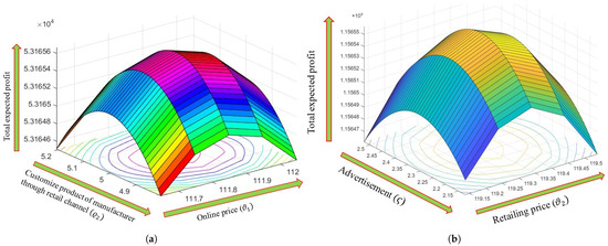
Figure 3.
Three-dimensional concavity curves for global maximum of the profit function with respect to the decision variables: (a) with respect to offline customized product of the manufacture and online price , where the evaluated range is 5.48–5.52 for and 111.65–112.05 for (CP method); (b) with respect to level of advertisement and retail price , where the evaluated range is 5.48–5.52 for and 125.87–126.27 for (VN method).
6.1. Discussion of Results
The results are discussed in detail in the following subsections.
6.1.1. Example for CP Method
In the CP problem, the total profit and optimum values of decision variables are = $53,165.67, = $126.07/unit, = $111.85/unit, = 23.01, = 5.62, = 4.19, = 4.8, = 6.23, = 6.53, = 5.01, and = 6.56. The selling price of the customized products in the online channel is less than that of the offline channel, i.e., . As for involvement in customized product design, the retailer involvement is more than the manufacturer’s online channel followed by the manufacturer’s offline channel, i.e., . As the majority of the total demand (80%) chooses the offline retail store, the retailer’s involvement for customized product design engages on the basis of customers’ satisfaction or service. In the case of cybersecurity, all SCN members’ involvement is more than 40%, but the offline channel requires more security than the online channel. For the online channel, customers do not carry cash and thus, the manufacturer does not require high security for transferring money from the store to the bank. This transportation is much riskier than cashless transaction. Because of that, the retailer is in a riskier position than the manufacturer; thus, the retailer’s involvement in cybersecurity is the highest. As the retailer already takes precautionary measures for cybersecurity, the manufacturer’s offline channel is less than the retailer but higher than the online channel, i.e., . Green innovation level of the manufacturer is 0.23% and the advertisement level of the retailer is 0.56%.
6.1.2. Example for VN Method
For the VN method, the manufacturer’s profit is $40,372.77. The selling price of the customized product in the online channel is 105.9 ($/unit). Then, the wholesale price of the manufacturer is 85.78 ($/unit). The green innovation level of the manufacturer is 0.187%. For cybersecurity, the level of engagement of the manufacturer is 0.039%, which is more in the online channel than the offline channel 0.036%, i.e., . For customized product design, the manufacturer’s engagement online is 0.0626% and the engagement offline is 0.0367%, i.e., .
The retailer’s profit is $11,565.56, and the product design engagement is 0.023%. The cybersecurity level is 0.0235%, advertisement level is 0.0232%, and the selling price is 117.81 ($/unit). The profitability is displayed in Table 3. The manufacturer’s profit is more than the retailer’s. The retailer’s engagement is less than the manufacturer’s in product design as well as cybersecurity level. In the case of VN, the cybersecurity level is more in the online channel than in the offline channel. Even for the offline channel, the manufacturer’s engagement in cybersecurity is more than the retailer. That is, the retailer’s cybersecurity level is the least among all channels. A concise executive summary of the result is given in Table 4.
Table 4.
Comparative discussion between CP and VN methods.
6.2. Special Cases
A few special cases are discussed for different circumstances. The results of the Special Cases I, II, and III are shown in Table 5 and Special Cases IV, V, VI, and VII are shown in Table 6. The analyses of parameters are categorized in two ways: constructive parameters and non-constructive parameters. Constructive parameters are discussed in detail within each of the special cases. Non-constructive parametric changes are summarized in Table 7 and Table 8.
- I.
- Constructive Parameter Discussions for Special Cases
6.2.1. Special Case I: Without Green Innovation
Under the same parameters, without green innovation, the overall profit for the CP method is = $48,357.13, and the optimal results in this scenario are = $115.47/unit, = $101.29/unit, = $8.27, = $3.78, = $4.48, = $5.83, = $6.04, = $4.64, and = $6.11. The profit in the CP method is 10.76% less than the original profit. For the VN method, the manufacturer’s profit is = $37,172.06, which is 7.93% less than the total profit of the manufacturer. The retailer’s profit is = $10,409.09, which is 10% less than the original retailer’s profit. This result demonstrates that without considering green innovation, the profit of SC decreases the most with respect to the original result, followed by the retailer and manufacturer. Therefore, the green innovation strategy is more profitable than not using it as a retailing strategy, especially for the CP method. As for the issue of long-term sustainability, this effect is not discussed in this manuscript. The following provides some analyses of constructive parameters and their range of convergence.
- For the CP method, the value of parameter a (base demand) has a lower limit of 21 units; that is, the minimum base demand for the customized product cannot be less than 21 units when there is no green innovation. If the base demand is less than 21 units, then the SCN incurs a loss, which belongs to both of the SC players. Hence, the industrial manager should focus on the base demand so that it is not less than 21 units in the case of no green innovation.
- The value of parameter (scaling parameter for selling price) has lower and upper limits of 10.49 and 98.91, respectively. For an value of 98.91 or more, the advertisement level decision variable becomes negative, and the profit becomes almost zero. For an value of 10.49, the online selling price is . For a value of either higher or lower than this, the online selling price increases excessively; all other decision variables and profit increase simultaneously. In reality, customers are not interested in buying a product for a high retail price. According to the real-life situation, a lower limit has been assigned for customer satisfaction. Hence, the industrial manager should focus on the parameter .
- The values of the parameters (scaling parameter for selling price of the other channel) and (scaling parameter for advertisement in demand) have an upper limits 11.91 and 11.61, respectively. For a value 11.91, the online selling price is $272.78, but for larger increases in , the retail price increases suddenly and excessively. For a value of 11.61, the online selling price and the advertisement level decision variable are $341.54 and $412, respectively, but for larger increases in the value of , the retail price and advertisement level decision variable increase excessively, imparting an effect upon the business. Hence, this is an important consideration for industrial managers.
- For the retailer in the VN method, the values of the parameters , , and have upper limits of 20.1, 49.99, and 21.7, respectively. For a value of 21.7, the values of the retail price and the advertisement level decision variable (> and , respectively) become excessively high. For an value of 20.1 or more, the advertisement and customized product design decision variables become negative, and the profit becomes less than $4.81. For a value of 20.1, the retail price becomes $261.78, but for larger increases in the value of , the retail price increases suddenly and excessively. On the other hand, the investment in advertisement, customized product, cybersecurity, and profit decrease simultaneously. Hence, industrial managers should focus on the condition of these parameters.
- For the manufacturer in the VN method, the value of parameter (scaling parameter for selling price) has lower and upper limits of 10.2 and 83, respectively. The value of parameter a (base demand) has a lower limit of 51 units. If the base demand is less than 51 units, then the business incurs a loss. Hence, industrial managers should focus on the base demand. That is, when the manufacturer maximizes its profit with its own decisions, the minimum base demand is 51 units, which is more than the CP method.
- The values of parameters (scaling parameter for selling price of the other channel) and (scaling parameter for advertisement on demand) have the upper limits 12.21 and 13.98, respectively. For a value of 13.98 or more, the value of the online price and the advertisement decision variable (> and ) become excessively high.
- For an value of 83 or more, the advertisement and customized product design decision variable become negative, and profit becomes almost zero. For an value of 10.2, the online selling price is . For higher or lower values, the online selling price increases excessively; all other decision variables and profit also increase suddenly. In reality, customers will not be interested in buying a product for a high retail price. According to the real-life situation, a lower limit has been assigned for customer satisfaction.
- For a value of 12.21, the retail price becomes $332.02, but for larger increases in the value of , the retail price increases excessively. Hence, the industrial manager should analyze those parameters properly.
Table 5.
Results of Special Cases I (no green innovation), II (no advertisement), and III (no cybersecurity).
6.2.2. Special Case II: Without Advertisement
Without advertisement effort and investment, the total profit for the CP method is = $52,356.46 and the optimal results are = $124.22/unit, = $110.3/unit, = 22.67, = 4.07, = 4.75, = 6.16, = 6.46, = 4.94, and = 6.48. This profit is 1.52% less than the original profit. For the VN method, the retailer’s profit is = $10,506.2, which is 9.16% less than the original profit. The manufacturer’s profit is = $40,075.31, which is 0.74% less than the original profit. The results find that the decentralized case faces more loss when there is no advertisement, and the retailer faces the most loss. The manufacturer faces the least loss when the manufacturer does not use advertisement. A wide analysis of the parameter’s range is given below.
- For the CP method, the value of the parameter (scaling parameter for selling price) has lower and upper limits of 10.71 and 98.54, respectively. For an value of 98.54 or more, the advertisement level decision variable becomes negative, and the profit becomes negligible. For an value of 10.71, the online selling price is . For higher or lower values of , the online selling price increases excessively; all other decision variables and profit increase simultaneously. In reality, customers are not interested in buying a product for a high retail price. Hence, the industrial manager should focus on the parameter .
- The value of the parameter a (base demand) has a lower limit of 20 units in the CP method. If the base demand is less than 20 units, then the business operates at a loss when there is no advertisement for the product. This limit is less than Case I, that is, when there is no green innovation. This implies that when the retailer does not invest in advertising, the base demand can go down than with no green innovation.
- The value of the scaling parameter for green innovation c and the scaling parameter for the selling price of the other channel have the upper limits 6.1 and 11.6, respectively. For c and values of 6.1 and 11.6, the online selling prices are $338.35 and $361.54, respectively, but for larger increases in the values of c and , the retail prices simultaneously increase excessively. Hence, the industrial manager should focus on the condition of these parameters.
- For the retailer in the VN method, the value of parameters (scaling parameter for selling price), c (scaling parameter for green innovation), and (scaling parameter for selling price of the other channel) have the upper limits 20.13, 168.91, and 11.19, respectively. For a c value of 168.91 or more, the value of the retail price (>) becomes excessively high. For an value of 20.13 or more, the green innovation and customized product design decision variable becomes negative, and the profit becomes less than $6.35. For a value of 11.19, the retail price becomes $282.76, but for larger increases in the value , the retail price increases suddenly and excessively. Hence, industrial managers should focus on the condition of these parameters.
- For the manufacturer in the VN method, the value of the scaling parameter for the selling price has lower and upper limits 10.42 and 83, respectively. For an value of 83 or more, the advertisement and customized product design decision variable become negative, and the profit is negligible. For an value of 10.42, the online selling price is . For higher or lower values of , the online selling price increases excessively; all other decision variables and profit also increase simultaneously. In reality, customers will not be interested in buying a product for a high retail price. According to the real-life situation, the lower limit has been assigned for customer satisfaction. Hence, the industrial manager should focus on the parameter .
- The value of the base demand a has a lower limit of 49 units. If the base demand is less than 49 units, then the business operates at a loss. That is, when each SC player decides their decision separately in the scenario without advertisement, the base demand is less than in Case I. No green innovation scenario has more base demand than the no advertisement scenario.
- The value of the scaling parameter for green innovation c and the scaling parameter for the selling price of the other channel have the upper limits 6.99 and 11.19, respectively. For c and values of and 6.99 and 11.19, the online selling prices are $338.35 and $361.54, respectively, but for larger increases in the values of c and , the retail price increases excessively and suddenly. Hence, industrial managers should focus on the condition of these parameters.
6.2.3. Special Case III: Without Cybersecurity
Without cybersecurity, the total profit for the CP method is = $52,105.58, and the optimal results in this scenario are = $123.69/unit, = $109.69/unit, = 22.56, = 8.88, = 6.43, = 4.92, and = 6.46. This profit without cybersecurity is 1.99% less than the original profit. For the VN method, the total profit of the retailer is = $11,433.02. The retailer’s profit without cybersecurity is 1.15% less than the original profit of the retailer. The manufacturer’s profit is = $39,815.83. It is 1.38% less than the original profit of the manufacturer. Based on this result, it can be determined that the profit of the CP method is more affected by the absence of cybersecurity than the decentralized policy. For the decentralized policy, the manufacturer faces more loss than the retailer. Therefore, the cybersecurity strategy is a good retailing strategy for all supply chain members. The ranges of different parameters are
- For the CP method, the value of the scaling parameter for the selling price has lower and upper limits of 10.4 and 99.3, respectively. For an value of 99.3 or more, the advertisement level decision variable becomes negative, and the profit is negligible. For an value of 10.4, the online selling price is . For higher or lower values of , the online selling price increases excessively; all other decision variables and profit increase suddenly. Hence, industrial managers should focus on the parameter .
- The value of the base demand a has a lower limit of 11 units. If the base demand is less than 21, then the business incurs a loss. Hence, industrial managers should focus on the base demand. The values of the parameters (scaling parameter for advertisement in demand), c (scaling parameter for green innovation), and (scaling parameter for selling price of the other channel) have the upper limits 11.1, 6, and 11.6, respectively.
- For a c value of 6, the online selling price and green level decision variable are $361.49 and $832.25, but for greater increases in the value c, the retail price and green level decision variable increase suddenly and excessively. For a value of 11.1, the online selling price is $363.48, but for larger increases in the value , the retail price increases suddenly and excessively. For a value of 11.6, the online selling price and the advertisement level decision variable are $345.87 and $461.63, respectively, but for larger increases in the value , the retail price and advertisement level decision variable increase excessively, imparting an effect upon business. Hence, this is an important consideration for industrial managers.
- For the retailer VN method, the value of parameters (scaling parameter for selling price), (scaling parameter for advertisement in demand), c (scaling parameter for green innovation), and (scaling parameter for selling price of the other channel) have the upper limits 20.34, 21.69, 171.01, and 11.18, respectively. For an value of 20.34 or more, the advertisement level decision variable becomes negative, and the profit becomes less than . For a value of 11.18, the retail price becomes , but for larger increases in the value , the retail price increases suddenly and excessively. For a value of 21.69 or more, the investment in advertisement and the selling price become minimum values of and , respectively.
- For a c value of 171.01 units or more in the CP method, the values of the retail price and green innovation investment have become minimum values of and . This implies that the base demand is feasible at 171.01 units, but the price and green innovation will become high. Thus, when there is no cybersecurity, the base demand is higher than in Cases I and II, but it should not be more than 171.01 units.
- For the manufacturer in the VN method, the value of the parameter (scaling parameter for selling price) has lower and upper limits of 10.4 and 83.6, respectively. For an value of 83.6 or more, the advertisement level decision variable becomes negative, and the profit is also near zero. For an value of 10.4, the online selling price is . For higher or lower values of , the online selling price increases excessively, all other decision variables and profit increase suddenly.
- The values of the parameters , c, and have upper limits of 13.75, 6.2, and 11.9, respectively. For a value of 11.9, the retail price becomes , but for larger increases in the value , the retail price increases excessively. For a c value of 6.2 or more, the values of the online price and the green level decision variable (> and ) become excessively high. For a value of 13.75 or more, the value of the online price and the advertisement level decision variable (> and ) become excessively high.
- The value of the base demand parameter a has a lower limit of 43 units in the VN method. If the base demand is less than 43 units, then the business operates at a loss. That is, decentralized decision-making has less value for the base demand of the manufacturer’s case than the retailer’s case. Hence, the effect of the retailer’s decision-making is more sensitive in the decentralized scenario without cybersecurity.
6.2.4. Special Case IV: Without Customized Product Design
Without customized product design, the total profit in the CP method is = $51,928.84 and the profit is 2.33% less the original profit in the CP method. For the VN method, the retailer’s profit is = $11,414.63 which is 1.28% less than the original profit of the retailer. The manufacturer’s profit = $39,627.19 is 1.85% less than the original manufacturer’s profit. It is found that the pattern of effect on supply chain members is similar to Special Case III, that is, no product design affects the centralized SCN than the decentralized policy. Ranges for some parameters are discussed below. The nature of all constrictive parameters are explained in this part.
- For the CP method, the value of the parameter has lower and upper limits of 10.7 and 99.5, respectively. For an value of 99.5 or more, the advertisement and customized product design decision variable become negative, and the profit becomes negligible. For an value of 10.7, the online selling price is . For higher or lower values of , the online selling price increases excessively; all other decision variables and profit also increase simultaneously. Hence, industrial managers should focus on the parameter .
- The value of the base parameter a has a lower limit of 14 units. If the base demand is less than 14, then the business operates at a loss. Hence, industrial managers should focus on the base demand. This scenario has a lower base demand than Cases, I, II, and III. Thus, when there is no customized product design for SCN, the market situation is more sensitive than without green innovation, cybersecurity, or advertisement.
- The values of parameters , c, and have upper limits of 11.14, 6.12, and 11.61, respectively. For a c value of 6.12, the online selling price and green level decision variable are $359.53 and $835.72, but for larger increases in the value c, the retail price and green level decision variable increase suddenly and excessively. For a value of 11.14, the online selling price is $358.76, but for larger increases in the value , the retail price increases suddenly and excessively. For a value of 11.61, the online selling price and the advertisement level decision variable are $341.71 and $462.64, respectively, but for larger increases in the value , the retail price and the advertisement level decision variable increase excessively, imparting an effect upon the business.
- For the retailer in the VN method, the values of the parameters , , c, and have upper limits of 20.33, 21.64, 171.21, and 11.18, respectively. For a c value of 171.21 or more, the values of the retail price and green innovation investment have become minimum values and . For an value of 20.33 or more, the advertisement level decision variable becomes negative, and the profit becomes less than .
- For a value of 11.18, the retail price becomes , but for larger increases in the value , the retail price suddenly increases excessively. For a value of 21.64 or more, the investment in advertisement and the selling price have become minimum values of and , respectively.
- For the manufacturer, the value of parameter has lower and upper limits of 10.21 and 83.73, respectively. For an value of 83.73 or more, the advertisement level decision variable becomes negative, and profit becomes almost zero. For an value of 10.21, the online selling price is . For higher or lower values of , the online selling price increases excessively, all other decision variables and profit also increase suddenly.
- The values of the parameters , c, and has upper limits of 13.72, 6.31, and 12, respectively. For a value of 12, the retail price becomes , but for larger increases in the value , the retail price increases excessively. For a c value of 6.31 or more, the value of the online price and the green level decision variable (> and ) become excessively high. For a value of 13.72 or more, the value of the online price and the advertisement level decision variable (> and ) become excessively high.
- The value of the base demand parameter a has a lower limit of 46 units. If the base demand is less than 46, then the business incurs a loss. Thus, when the manufacturer makes a decision, the minimum base demand should not be more than 46 units. Hence, industrial managers should focus on the behavior of these parameters.
Table 6.
Table for Special Cases IV (no customized product design), V (no customized product design by the retailer), VI (no customized product design in online channel by the manufacturer), and VII (no customized product design by the manufacturer (offline)).
6.2.5. Special Case V: Without Customized Product Design by the Retailer in Offline Channel
Without customized product design by the retailer in the offline channel only, the overall profit for the CP method is = $52,653.33. The profit is 0.96% less than the original profit of the SCN in the CP method. For the VN method, the retailer’s profit is = $11,546.46. The retailer faces a 0.17% loss compared to the original profit. The manufacturer has a profit of = $40,169.51, which is 0.5% less than the original profit in the VN method. Even if the retailer is not the only supply chain member who does not invest in the product design, the retailer is the least loss-facing member. Other members pay for the product design. However, the CP method faces the most loss among all methods. Associated ranges of the parameters are given below.
- For the CP method, the value of the parameter has lower and upper limits of 10.7 and 98.6, respectively. For an value of 98.54 or more, the advertisement and customized product design decision variable become negative, and the profit is approximately zero. For an value of 10.71, the online selling price is . For higher or lower values of , the online selling price increases excessively; all other decision variables and profit increase simultaneously. Hence, industrial managers should focus on the parameter .
- The value of the base demand parameter a has a lower limit of 18 units. If the base demand is less than 18, then the business operates at a loss in the CP method. Thus, the SCN players should consider the minimum base demand of 18 units when there is no customized product design by the retailer. Hence, industrial managers should focus on the base demand.
- The values of parameters , c, and have upper limits of 11.6, 6.01, and 10.99, respectively. For a c value of 6.01, the online selling price and green level decision variable are $355.82 and $833.23, but for larger increases in the value of c, the retail prices and green level decision variable increase suddenly and excessively. For a value of 10.99, the online selling prices are $356.61, but for greater increases in the value , the retail prices increase suddenly and excessively.
- For a value of 11.6, the online selling price and the advertisement level decision variable are $339.09 and $459.59, respectively, but for larger increases in the value , the retail price and advertisement level decision variable increase excessively, imparting an effect upon the business. Hence, this is important for industrial managers.
- For the retailer in the VN method, the values of the parameters , , c, and have upper limits of 20.06, 21.69, 171.01, and 11.05, respectively. For a c value of 171.01 or more, the value of the retail price and green innovation investment have become minimum values of and . For an value of 20.06 or more, the advertisement level decision variable becomes negative and profit becomes less than .
- For a value of 11.05, the retail price becomes , but for much greater increases in the value , the retail price suddenly increases excessively. For a value of 21.69 or more, the investment in advertisement and selling prices has become a minimum of and , respectively. Hence, industrial managers should focus on the condition of these parameters.
- For the manufacturer in the VN method, the values of parameters have lower and upper limits of 10.4 and 83.96, respectively. For an value of 83.96 or more, the advertisement and customized product design decision variable become negative, and the profit is also near zero. For an value of 10.4, the online selling price is . For higher or lower values of , the online selling price increases excessively; all other decision variables and profit also increase simultaneously. Hence, industrial managers should focus on the parameter .
- The value of the base demand parameter a has a lower limit of 46 units. If the base demand is less than 46 units, then the business operates at a loss. Hence, industrial managers should focus on the base demand. The values of the parameters , c, and have upper limits of 11.97, 6.2, and 13.79, respectively.
Table 7.
Comparative discussions for non-constructive parameters in Special Cases I, II, III, and IV.
6.2.6. Special Case VI: Without Customized Product Design by the Manufacturer Through Online Channel
Without product design by the manufacturer in the online channel, the overall profit for the CP method is = $52,705.45; this is 0.87% less than the original profit in the CP method. For the VN method, the retailer’s profit is = $11,549.95, which is 0.11% less than the original profit of the retailer in the VN method. = $39,948.39 is the profit of the manufacturer in the VN method, which is 1.05% less than the manufacturer’s profit in the VN method. It is found that without considering customized products by the manufacturer through online channels, the manufacturer loses the most, followed by the retailer when using the CP method. Thus, unless the retailer uses the offline channel, the manufacturer faces the maximum loss when the manufacturer does not consider product design. Ranges of some parameters are described below.
- For the CP method, the value of the parameter has lower and upper limits of 10.7 and 99.21, respectively. For an value of 99.21 or more, the advertisement and customized product design decision variable become negative, and the profit decreases towards zero. For an value of 10.71, the online selling price is . For higher or lower values of , the online selling price increases excessively; all other decision variables and profit also increase simultaneously. Hence, industrial managers should focus on the parameter .
- The value of the base demand parameter a has a lower limit of 19 units. If the base demand is less than 19 units, then the business incurs a loss. Thus, when the manufacturer does not use product customization online, then the SCN base demand should be more than 19 units. Hence, industrial managers should focus on base demand.
- The values of parameters , c, and have upper limits of 11.61, 6.98, and 11.16, respectively. For a c value of 6.98, the online retail price and green level decision variable are $358.22 and $834.96, but for greater increases in the value of c, the retail prices and green level decision variable increase suddenly and excessively.
- For a value of 11.16, the online selling price is $358.01, but for larger increases in the value , the retail price suddenly increases excessively. For a value of 11.61, the online selling prices and the advertisement level decision variable are $341.98 and $458.05, respectively, but for larger increases in the value , the retail prices and advertisement level decision variable increase excessively, imparting an effect upon the business.
- For the retailer in the VN method, the values of the parameters , , c, and have upper limits of 20.09, 21.71, 169.85, and 11.19, respectively. For a c value of 169.85 or more, the value of the retail price and green innovation investment have become minimum values of and . In reality, the customer will not be interested in buying the product for a high retail price. For an value of 20.09 or more, the advertisement level decision variable becomes negative, and profit becomes less than .
- For a value of 11.19, the retail price becomes , but for larger increases in the value of , the retail price increases suddenly and excessively. For a value of 21.71 or more, the investment in advertisement and selling prices has become a minimum of and , respectively. In reality, the customer will not be interested in buying the product for a high retail price. According to the real-life field scenario, an upper limit has been assigned for customer satisfaction. Hence, industry managers should focus on the conditions of these parameters.
- For the manufacturer in the VN method, the value of the parameter has lower and upper limits of 10.4 and 83.45, respectively. For an value of 83.45 or more, the advertisement level decision variable becomes negative, and the profit is almost zero. For an value of 10.4, the online selling price is . For higher or lower values of , the online selling price increases excessively; all other decision variables and profit also increase suddenly. In reality, customers will not be interested in buying the product for a high retail price.
- The value of the parameters , c, and have upper limits of 11.96, 6.2, and 13.69, respectively. For a value of 11.96, the retail price becomes , but for larger increases in the value , the retail price increases excessively. For a c value of 6.2 or more, the value of the online price and the green level decision variable (> and ) become excessively high. For a value of 13.69 or more, the value of the online price and the advertisement level decision variable (> and ) become excessively high. The value of the base demand parameter a has a lower limit of 49 units. If the base demand is less than 49 units, then the business operates at a loss. Hence, industrial managers should focus on the behavior of those parameters.
Table 8.
Comparative discussions for non-constructive parameters in Special Cases V, VI, and VII.
6.2.7. Special Case VII: Without Customized Product Design of the Manufacturer Through Offline Channel
Without customized product design by the manufacturer in the offline channel, the overall profit for the CP method is = $52,883.26. This is 0.53% less than the original CP profit. For the VN method, the retailer’s profit is = $11,447.19, which is 1.02% less profitable than in the VN method in offline channel. The manufacturer’s profit is = $40,247.33, which is 0.31% less than the original profit in the VN method through offline channel; that is, without considering product customization by manufacturer through the offline channel, the loss to the manufacturer is more than the retailer when using the CP method. Ranges of several parameters are given below.
- For the CP method, the value of the parameter has lower and upper limits of 10.6 and 98.63, respectively. For an value of 98.63 or more, the advertisement level decision variable becomes negative, and the profit is negligible. For an value of 10.6, the online selling price is . For higher or lower values of , the online selling price increases excessively; all other decision variables and profit also increase simultaneously. In reality, customers will not be interested in buying the product for a high retail price.
- The value of the base demand parameter a has a lower limit of 18 units. If the base demand is less than 18, then the business operates at a loss. Hence, industrial managers should focus on the base demand. The values of the parameters , c, and have upper limits of 11.59, 6.05, and 11, respectively. For a c value of 6.05, the online selling price and green level decision variable are $357.92 and $836.06, but for larger increases in the value c, the retail prices and green level decision variable increase suddenly and excessively.
- For a value of 11, the online selling prices are $367.84, but for larger increases in the value , the retail prices increase suddenly and excessively. For a value of 11.59, the online selling prices and the advertisement level decision variable are $343.05 and $460.71, respectively, but for larger increases in the value , the retail prices and advertisement level decision variable increase excessively, imparting an effect upon the business. Hence, this is an important consideration for industrial managers.
- For the retailer in the VN method, the values of the parameters , , c, and have upper limits of 20.14, 21.71, 171.02, and 11.19, respectively. For a c value of 171.02 or more, the value of the retail price and green innovation investment have become minimum values of and . For an value of 20.14 or more, the advertisement level decision variable becomes negative and profit becomes less than .
- For a value of 11.19, the retail price becomes , but for larger increases in the value , the retail price increases suddenly and excessively. For a value of 21.71 or more, the investment in advertisement and the selling price become minimum values of and , respectively.
- For the manufacturer in the VN method, the value of the parameter has lower and upper limits of 10.4 and 83.8, respectively. For an value of 83.8 or more, the advertisement level decision variable becomes negative, and the profit is also near zero. For an value of 10.4, the online selling price is . For higher or lower values of , the online selling price increases excessively; all other decision variables and profit also increase suddenly.
- The values of the parameters , c, and have upper limits of 11.99, 6.18, and 13.68, respectively. For a value of 11.99, the retail price becomes , but for larger increases in the value , the retail price increases excessively. For a c value of 6.18 or more, the value of the online price and the green level decision variable (> and ) become excessively high. For a value of 13.68 or more, the value of the online price and the advertisement level decision variable (> and ) become excessively high. The value of the base demand parameter a has a lower limit of 48 units. If the base demand is less than 48 units, then the business operates at a loss. Hence, the industrial manager should focus on the behavior of those parameters.
- II.
- Nonconstructive Parameter Discussions for Special Cases
The natures of all nonconstructive investment parameters for Special Cases I, II, III, IV, V, VI, and VII are explained in Table 7 and Table 8. These tables explain the associative investment thresholds. The parameters are increased by up to 9900% and decreased by up to 99%. For all the cases, the following patterns are found.
- A maximum decrease of 99% in the investment parametric values increases the profit significantly. However, for small changes such as 5% or 10%, the profit changes are insignificant.
- The results in Table 7 and Table 8 imply that an investment that is significantly higher than the optimum value reduces the relevant decision activities by the SC player. Those tasks are automatically taken care of by the associative setup. But, the investment should not be much lower than the optimized value for the stability of the result.
- For Special Case II, when there is no advertisement by the retailer, the green innovation investment parameter decreases to 90%, not to 99%. That is, without investment, green investment can be relaxed to 90% but not less than that.
- It is found that when advertisement is withdrawn from the system, it causes the maximum profit loss, −8.84%, when the green investment parameter is increased to 9900%; this is the highest among all special cases. Similarly, a −90% causes a 65.25% increase in profit, which is again the highest among all cases.
6.3. Discussions and Comparisons
Figure 4 compares the profit between the CP and VN methods. According to Table 3 and Figure 4, the maximum profit between the two policies is obtained under the CP method, which is $53,165.67. From all the Special Cases, no use of green innovation in Special Case I has the highest effect on the SCN profit (Table 5) in the CP method, followed by the VN method.
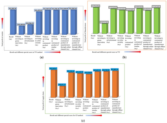
Figure 4.
Graphical presentation of result and special cases: (a) retailer in the VN method, (b) manufacturer in the VN method, and (c) supply chain in CP method.
For the purpose of this study, numerical comparisons to the existing literature are shown in Table 9. Pal et al. [60] studied green innovation and promotional effort. However, their research neglected customized products and cybersecurity. They obtained profits of $16,237.2 and $14,567.90 for the CP and VN methods, respectively, which are 69.45% and 71.95% less than the profits obtained in this study, respectively. Kar et al. [61] studied a dual-channel strategy, advertisement, and green innovation, but their research did not consider customized products and cybersecurity policies. The profit in the CP method was $2226.93, which 95.81% less than that obtained in this study. They did not consider a decentralized policy.
Table 9.
Comparison with previous findings in the academic literature.
6.4. Sensitivity Analysis
To analysis the solutions, sensitivity analysis has been performed. Sensitivity analyses are shown in the tornado chart in Figure 5 and Table 10. This examines the impact of altering a parameter between the range of to .
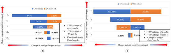
Figure 5.
Tornado graph for a comparison of sensitivity analyses: (a) +25% changes for a and c and +10% changes for and in CP and VN methods; (b) +50% changes for , , and and +20% changes for and in CP and VN methods.
- is the most sensitive parameter, which is the cross-selling parameter. With a 10% positive change, it elevates the profits by 103.69% in the CP method and 86.3% in the VN method. For 20% changes, the VN methods provides changes, but the CP method diverges; that is, the CP method is more sensitive than VN method.
- The base demand is the next-most sensitive parameter. A decrement in a decreases profit of the supply chain by , and an increase of a increases the total supply chain profit by . The effect on the retailer’s profit is greater in offline channel than in the other cases.
- Greenness level is also a very sensitive parameter. Out of the two policies, in the CP method, the greenness level (c) has more impact on the total profit. A decrease of in greenness level decreases the total profit by , and an increase of increases the total profit by . c is more sensitive for the retailer in the VN method. The parameter c is similarly sensitive for other cases.
- The parameter related to the cybersecurity of the retailer () is more sensitive than the manufacturer’s cybersecurity parameter (). Out of these policies, the CP method shows the greatest amount of variation. A increment in and increases profit by and , respectively, whereas a decrement in and decreases the profit by and , respectively.
- is one of the most sensitive parameters, as it only varies between 10% to 20%. In the centralized and VN method, the parameter is too sensitive, decreases greater than 10% causes divergence in the results.
- The variable transportation cost of the manufacturer () is a more sensitive parameter than the variable transportation cost of the retailer (). The transportation cost of the manufacturer does not affect the retailer’s profit in the VN method. In the VN method, is much less sensitive, but in the CP Method, is a sensitive parameter. The effects of and are negligible.
Table 10.
Sensitivity analysis of principal parameters in the VN and CP methods.
7. Managerial Interpretation and Insights
In this section, managerial interpretation and insights are discussed separately in two subsections.
7.1. Business Interpretation with an Example
An example of a real-life scenario can help better understand the relationship between the present study and real business cases.
- An electronics manufacturer produces Bluetooth headphones. They use both online and offline channels for business.
- However, the manufacturer is not available offline in the market, especially for consumers. The manufacturer only opens sales for consumers through the online channel. The manufacturer sells Bluetooth headphones to retailers through offline channels.
- In that case, consumers can buy products according to their choice due to their ability to provide customized products. The online sales channel is operated by the manufacturer, and the offline sales channel is operated by the retailer.
- Customized product design is available for consumers from both channels, i.e., online and offline. The retailer passes the customization request to the manufacturer for the offline channel, and the manufacturer directly receives the Bluetooth headphone customization request from consumers.
- The Bluetooth headphones have a long-lasting battery that reduces the number of charges. This reduces carbon footprint for environmental sustainability.
- Since Bluetooth headphones connect through mobile or web applications, the electronics company prioritizes data protection, secure connectivity, and regular software updates for applications. This is categorized as cybersecurity, which builds consumers’ trust, reduces the risk of cyber threats, and protects both users’ and the electronics company’s reputation.
7.2. Managerial Insights
Some recommendations for managers are listed below.
- Industrial managers are advised to open a new policy named customized product service through dual channels. This is because by satisfying a customer and meeting their needs, managers can improve the business according to the customer’s experience and taste [62]. As a result, the company can increase the brand’s value in the competitive market and can earn maximum profit.
- Industrial managers should take care of the customer’s loyalty and trust by securing the customer’s data safety and avoiding interrupted operations. Therefore, manufacturers should invest in cybersecurity to maintain brand value in the market and retain the same trust between all supply chain members.
- Embracing green practices not only minimizes environmental footprint but also enhances the brand image and customer confidence. Managers must see green endeavors as strategic investments that can generate cost savings, regulatory conformance, and competitive advantages.
- Providing both online and offline channels increases customer convenience and market coverage. Managers need to carefully balance the prices, inventories, and quality of services across the channels to prevent conflict and provide consistency. Using data from both channels offers greater consumer insight and allows personalized approaches. Properly integrating dual channels leads to stronger loyalty among customers and sustainable business growth.
- Managers need to spend advertising funds efficiently by approaching the appropriate market segments to achieve maximum return on investment. Combining traditional and digital platforms ensures broader reach and flexibility in response to shifts in consumer behavior. Finally, ongoing assessment of the effectiveness of advertisements allows refining of strategies and maintaining a long-term competitive edge.
8. Conclusions
An SCN model was developed where the manufacturer and the retailer were the supply chain members. The model was developed with customized product, cybersecurity, green innovation, dual-channel retailing, and advertisement, which contribute significantly to the industry by maximizing the total profit.
- The study indicated that customized products enhance brand loyalty, and robust security practices minimized data breaches and business risks.
- It was found that the CP method always provided increased profit over the VN method, i.e., centralized policy is better than decentralized policy.
- When the manufacturer did not invest in green innovation, then the system’s profit reduced the most among all methods. Without investing in customized products and cybersecurity, the profit of the supply chain decreased by 2.36% in the centralized method, which is the most among the CP and VN methods.
This study can be extended in various directions. Investigating long-term sustainability issues for the implementation of green innovation is an immediate extension [63,64]. It can be extended for deteriorating products by considering preservation technology [65]. Uncertainty methodologies such as fuzzy logic [66] and metaheuristic approaches can be used to extend this study. It can be extended using home delivery policy to obtain an advantage over the competition [67]. Customer care support for service can be used [68] as an extension.
Author Contributions
Conceptualization, data curation, P.M. and M.S.; methodology, R.G. and M.S.; writing of original draft, P.M.; software, P.M., S.P., B.K.D., and R.G.; resources, review and editing, P.M., S.P., A.G., and M.S.; validation, M.S., B.K.D., and R.G.; visualization, formal analysis, B.K.D., R.G., M.S., and A.G.; supervision S.P.; investigation, S.P., M.S., B.K.D., and R.G. All authors have read and agreed to the published version of the manuscript.
Funding
This research received no external funding.
Data Availability Statement
The original contributions presented in this study are included in the article. Further inquiries can be directed to the corresponding authors.
Conflicts of Interest
The authors declare no conflicts of interest.
Appendix A
Table A1.
All parameters that are used in the special cases and sensitivity analysis.
Appendix B
All derivatives in this appendix are here.
All other partial derivatives are zero. This research endeavor assesses the globally optimal solution through the utilization of a Hessian matrix (H) within the framework of a CP method.
The first-order principal minor of a Hessian matrix is . The second-order principal minor of a Hessian matrix is
The third-order principal minor of a Hessian matrix is
= − + . The fourth-order principal minor of a Hessian matrix is
= . As . The fifth-order principal minor of a Hessian matrix is =
and . The sixth-order principal minor of a Hessian matrix is =
= . As and . The seventh-order principal minor of a Hessian matrix is =
= . As and . The eighth-order principal minor of an Hessian matrix is =
= . As and . The ninth-order principal minor of a Hessian matrix is =
= . As and . The tenth-order principal minor of a Hessian matrix is = = . As and .
Appendix C
Two Appendices are discussed in this section.
Appendix C.1
All first- and second-order partial derivatives that is needed in the Hessian matrix for manufacturer in the VN method.
All other partial derivatives are zero. The Hessian matrix of this appendix is =
The first-order principal minor of a Hessian matrix is , if . The second-order principal minor of a Hessian matrix is
and . The third-order principal minor of a Hessian matrix is =
If + , i.e., and as . The fourth-order principal minor of Hessian matrix of is =
As , and, . The fifth-order principal minor of a Hessian matrix is =
and . The sixth-order principal minor of a Hessian matrix is = = () . = and .
Appendix C.2
All first- and second-order partial derivatives that are needed for the retailer in H in the VN method.
Other partial derivatives are zero. The Hessian matrix H of this appendix is =
The first-order principal minor of a Hessian matrix is if . The second-order principal minor of a Hessian matrix is
and . The third-order principal minor of a Hessian matrix is =
If , i.e., and as . The fourth-order principal minor of a Hessian matrix is = and .
References
- Monaro, M.; Bettelli, A.; Portello, G.; Pierobon, L.; Orso, V.; Caputo, A.; Campanini, M.L.; Giachetti, A.; Gamberini, L. Enhancing shopping experience in augmented reality by customizing product manipulation modalities: A customer experience study. Int. J. Hum. Comput. Stud. 2025, 202, 103553. [Google Scholar] [CrossRef]
- Frutos, J.D.; Borenstein, D. A framework to support customer company interaction in mass customization environments. Comput. Ind. 2004, 54, 115–135. [Google Scholar] [CrossRef]
- Sarkar, B.; Sao, S.; Ghosh, S.K. Smart production and photocatalytic ultraviolet (PUV) wastewater treatment effect on a textile supply chain management. Int. J. Prod. Econ. 2025, 283, 109557. [Google Scholar] [CrossRef]
- Safitra, M.F.; Lubis, M.; Fakhrurroja, H. Counterattacking cyber threats: A framework for the future of cyber security. Sustainability 2023, 15, 13369. [Google Scholar] [CrossRef]
- Unsal, O. Corporate crimes and innovation: Evidence from US financial firms. Econ. Model. 2023, 120, 106183. [Google Scholar] [CrossRef]
- Adhikari, A.; Basu, S.; Avittathur, B. Greening innovation, advertising, and pricing decisions under competition and market coverage. J. Clean. Prod. 2025, 494, 144951. [Google Scholar] [CrossRef]
- Trentin, A.; Forza, C.; Perin, E. Embeddedness and path dependence of organizational capabilities for mass customization and green management: A longitudinal case study in the machinery industry. Int. J. Prod. Econ. 2015, 169, 253–276. [Google Scholar] [CrossRef]
- Olsen, G.D.; Pracejus, J.W. Customized advertising: Allowing consumers to directly tailor messages leads to better outcomes for the brand. J. Bus. Res. 2020, 116, 245–257. [Google Scholar] [CrossRef]
- Moon, I.; Yun, W.Y.; Sarkar, B. Effects of variable setup cost, reliability, and production costs under controlled carbon emissions in a reliable production system. Eur. J. Ind. Eng. 2022, 16, 371–397. [Google Scholar] [CrossRef]
- He, B.; Ozdemir Akyildirim, O.; Yuan, K. Product customization schemes and value co-creation with platform driven C2M model. Electron. Commer. Res. Appl. 2023, 62, 101339. [Google Scholar] [CrossRef]
- Singh, S.K.; Chauhan, A.; Sarkar, B. Sustainable biodiesel supply chain model based on waste animal fat with subsidy and advertisement. J. Clean. Prod. 2023, 382, 134806. [Google Scholar] [CrossRef]
- Du, B.; Yuan, J.; Shu, W.; Shen, Y. Optimal product customization and cooperative advertising strategies in supply chain with social influence. Procedia Comput. Sci. 2023, 221, 992–999. [Google Scholar] [CrossRef]
- Chauhan, R.; Majumder, A.; Kumar, V. The impact of adopting customization policy and sustainability for improving consumer service in a dual channel retailing. J. Retail. Consum. Serv. 2023, 75, 103504. [Google Scholar] [CrossRef]
- Gautam, P.; Maheshwari, S.; Kausar, A.; Jaggi, C.K. Sustainable retail model with preservation technology investment to moderate deterioration with environmental deliberations. J. Clean. Prod. 2023, 390, 136128. [Google Scholar] [CrossRef]
- Battaglini, F. Will the European green deal enhance Europe’s security towards Russia? A political economy perspective. Energy Econ. 2024, 134, 107551. [Google Scholar] [CrossRef]
- Song, J.M.; Wang, T.; Yen, J.C.; Chen, Y.H. Does cyber security maturity level assurance improve cyber security risk management in supply chains? Int. J. Account. Inf. Syst. 2024, 54, 100695. [Google Scholar] [CrossRef]
- Mahapatra, A.S.; Sengupta, S.; Dasgupta, A.; Sarkar, B.; Goswami, R.T. What is the impact of demand patterns on integrated online offline and buy online pickup in store (BOPS) retail in a smart supply chain management? J. Retail. Consum. Serv. 2025, 82, 104093. [Google Scholar] [CrossRef]
- Liu, L.; Xu, J.; Fang, J.; Sun, G. Research on optimization of distributed network security framework based on blockchain under green computing framework. Sustain. Comput. Inform. Syst. 2025, 48, 101183. [Google Scholar] [CrossRef]
- Chauhan, R.; Majumder, A. Involvement of carbon regulation in a smart dual channel supply chain for customized products under uncertain environment. Environ. Dev. Sustain. 2025, 27, 6997–7032. [Google Scholar] [CrossRef]
- Zhang, J.; Wu, D. How to design channel structures in the dual channel supply chain with sequential entry of manufacturers? Comput. Ind. Eng. 2022, 169, 108234. [Google Scholar] [CrossRef]
- Huang, Y.; Ho, J.; Wu, G. A study on promotion with strategic two stage customized bundling. J. Retail. Consum. Serv. 2022, 68, 103004. [Google Scholar] [CrossRef]
- Flacandji, M.; Vlad, M.; Lunardo, R. The effects of retail apps on shopping well being and loyalty intention: A matter of competence more than autonomy. J. Retail. Consum. Serv. 2024, 78, 103762. [Google Scholar] [CrossRef]
- Wang, J.; Jiang, H.; Yu, M. Pricing decisions in a dual channel green supply chain with product customization. J. Clean. Prod. 2020, 247, 119101. [Google Scholar] [CrossRef]
- Zhang, T.; Tang, Z. Should manufacturers open live streaming shopping channels? J. Retail. Consum. Serv. 2023, 71, 103229. [Google Scholar] [CrossRef]
- Kim, H.; Ryu, M.H.; Lee, D.; Kim, J.H. Should a small sized store have both online and offline channels? An efficiency analysis of the O2O platform strategy. J. Retail. Consum. Serv. 2022, 64, 102823. [Google Scholar] [CrossRef]
- Pan, Z.; Wang, Z.; Qiu, L.; Zhang, S.; Zhu, H.; Zhang, H.; Xiang, F.; Cheng, C. ConfigRec: An efficient recommendatory configuration design method for customized products. J. Manuf. Syst. 2025, 82, 161–177. [Google Scholar] [CrossRef]
- Hosseini-Motlagh, S.M.; Johari, M.; Pazari, P. Coordinating pricing, warranty replacement and sales service decisions in a competitive dual channel retailing system. Comput. Ind. Eng. 2022, 163, 107862. [Google Scholar] [CrossRef]
- Lu, F.; Lian, Y.; Sun, W.; Min, X.; Zhai, G. A study on the user viewing experience of implanted advertisement videos based on visual saliency. Expert Syst. Appl. 2025, 291, 128499. [Google Scholar] [CrossRef]
- Mirzagoltabar, H.; Shirazi, B.; Mahdavi, I.; Khamseh, A.A. Sustainable dual channel closed loop supply chain network with new products for the lighting industry. Comput. Ind. Eng. 2021, 162, 107781. [Google Scholar] [CrossRef]
- Zhang, C.; Li, Y.; Ma, Y. Direct selling, agent selling, or dual format selling: Electronic channel configuration considering channel competition and platform service. Comput. Ind. Eng. 2021, 157, 107368. [Google Scholar] [CrossRef]
- Qiu, R.; Hou, L.; Sun, Y.; Sun, M.; Sun, Y. Joint pricing, ordering and order fulfillment decisions for a dual channel supply chain with demand uncertainties: A distribution free approach. Comput. Ind. Eng. 2021, 160, 107546. [Google Scholar] [CrossRef]
- Nishio, K.; Hoshino, T. Quantifying the short and long term effects of promotional incentives in a loyalty program: Evidence from birthday rewards in a large retail company. J. Retail. Consum. Serv. 2024, 81, 103957. [Google Scholar] [CrossRef]
- Pei, Z.; Yan, R. National advertising, dual channel coordination and firm performance. J. Retail. Consum. Serv. 2013, 20, 218–224. [Google Scholar] [CrossRef]
- Sarkar, B.; Singh, S.K.; Chauhan, A. An advanced robust possibilistic chance constrained programming model for the animal fat based biodiesel supply chain network. J. Ind. Inf. Integr. 2025, 47, 100884. [Google Scholar] [CrossRef]
- Gao, Y.; Lu, S.; Cheng, H.; Liu, X. Data driven robust optimization of dual channel closed loop supply chain network design considering uncertain demand and carbon cap and trade policy. Comput. Ind. Eng. 2024, 187, 109811. [Google Scholar] [CrossRef]
- Kumar, S.; Sigroha, M.; Kumar, N.; Kumari, M.; Sarkar, B. How does the retail price maintain trade credit management with continuous investment to support the cash flow? J. Retail. Consum. Serv. 2025, 83, 104116. [Google Scholar] [CrossRef]
- Chaudhari, U.; Bhadoriya, A.; Jani, M.Y.; Sarkar, B. A generalized payment policy for deteriorating items when demand depends on price, stock, and advertisement under carbon tax regulations. Math. Comput. Simul. 2023, 207, 556–574. [Google Scholar] [CrossRef]
- Motlagh, P.H.; Nasiri, G.R. Developing a pricing strategy and coordination in a dual channel supply chain incorporating inventory policy and marketing considerations. Comput. Ind. Eng. 2023, 185, 109607. [Google Scholar] [CrossRef]
- Benmalek, M. Ransomware on cyber physical systems: Taxonomies, case studies, security gaps, and open challenges. Internet Things Cyber Phys. Syst. 2024, 4, 186–202. [Google Scholar] [CrossRef]
- Govindarajan, U.H.; Singh, D.K.; Gohel, H.A. Forecasting cyber security threats landscape and associated technical trends in telehealth using Bidirectional Encoder Representations from Transformers (BERT). Comput. Secur. 2023, 133, 103404. [Google Scholar] [CrossRef]
- Jana, D.K.; Ghosh, R. Novel interval type-2 fuzzy logic controller for improving risk assessment model of cyber security. J. Inf. Secur. Appl. 2018, 40, 173–182. [Google Scholar] [CrossRef]
- Li, L.; Yan, S.; Peng, S.; Hou, P. The interplay of blockchain and channel structure with consideration of cyber-security in a platform supply chain. Transp. Res. Part E Logist. Transp. Rev. 2025, 197, 104045. [Google Scholar] [CrossRef]
- Wang, S.S. Integrated framework for information security investment and cyber insurance. Pac. Basin Financ. J. 2019, 57, 101173. [Google Scholar] [CrossRef]
- Gombár, M.; Vagaská, A.; Korauš, A.; Račková, P. Application of structural equation modelling to cyber security risk analysis in the era of industry 4.0. Mathematics 2024, 12, 343. [Google Scholar] [CrossRef]
- Tayyab, M.; Habib, M.S.; Jajja, M.S.S.; Sarkar, B. Economic assessment of a serial production system with random imperfection and shortages: A step towards sustainability. Comput. Ind. Eng. 2022, 171, 108398. [Google Scholar] [CrossRef]
- Rajabion, L.; Khorraminia, M.; Andjomshoaa, A.; Ghafouri Azar, M.; Molavi, H. A new model for assessing the impact of the urban intelligent transportation system, farmers? Knowledge and business processes on the success of green supply chain management system for urban distribution of agricultural products. J. Retail. Consum. Serv. 2019, 50, 154–162. [Google Scholar] [CrossRef]
- Samanta, S.; Dubey, V.K.; Sarkar, B. Measure of influences in social networks. Appl. Soft Comput. 2021, 99, 106858. [Google Scholar] [CrossRef]
- Saen, R.F.; Karimi, B.; Fathi, A. Unleashing efficiency potential: The power of non convex double frontiers in sustainable transportation supply chains. Socio Econ. Plan. Sci. 2025, 98, 102143. [Google Scholar] [CrossRef]
- Sherif, S.U.; Asokan, P.; Sasikumar, P.; Mathiyazhagan, K.; Jerald, J. Integrated optimization of transportation, inventory and vehicle routing with simultaneous pickup and delivery in two echelon green supply chain network. J. Clean. Prod. 2021, 287, 125434. [Google Scholar] [CrossRef]
- Nugroho, Y.K.; Zhu, L. Strategic supply and transportation planning of a supply chain for agricultural biomass to hydrogen and syngas. Comput. Ind. Eng. 2024, 197, 110640. [Google Scholar] [CrossRef]
- Tayyab, M.; Sarkar, B. An interactive fuzzy programming approach for a sustainable supplier selection under textile supply chain management. Comput. Ind. Eng. 2021, 155, 107164. [Google Scholar] [CrossRef]
- Yige, Z.; Haibo, K.; Min, W.; Meng, Z.; Jianzhao, L. Research on government subsidy strategy of green shipping supply chain considering corporate social responsibility. Res. Transp. Bus. Manag. 2025, 60, 101368. [Google Scholar] [CrossRef]
- Debnath, A.; Sarkar, B. Effect of circular economy for waste nullification under a sustainable supply chain management. J. Clean. Prod. 2023, 385, 135477. [Google Scholar] [CrossRef]
- Alamri, O.A.; Lamba, N.K.; Jayaswal, M.K.; Mittal, M. A sustainable inventory model with advertisement effort for imperfect quality items under learning in fuzzy monsoon demand. Mathematics 2024, 12, 2432. [Google Scholar] [CrossRef]
- Habib, M.S.; Omair, M.; Ramzan, M.B.; Chaudhary, T.N.; Farooq, M.; Sarkar, B. A robust possibilistic flexible programming approach toward a resilient and cost efficient biodiesel supply chain network. J. Clean. Prod. 2022, 366, 132752. [Google Scholar] [CrossRef]
- Ahmed, W.; Moazzam, M.; Sarkar, B.; Rehman, S.U. Synergic effect of reworking for imperfect quality items with the integration of multi period delay in payment and partial backordering in global supply chains. Engineering 2021, 7, 260–271. [Google Scholar] [CrossRef]
- Yadav, D.; Singh, R.; Kumar, A.; Sarkar, B. Reduction of pollution through sustainable and flexible production by controlling by-products. J. Environ. Inform. 2022, 40, 106–124. [Google Scholar] [CrossRef]
- Levi-Bliech, M.; Dahan, G. The impact of green innovation products on an organization’s social performance via green supply chain management. Green Technol. Sustain. 2025, 4, 100273. [Google Scholar] [CrossRef]
- Guchhait, R.; Sarkar, B. A decision making problem for product outsourcing with flexible production under a global supply chain management. Int. J. Prod. Econ. 2024, 272, 109230. [Google Scholar] [CrossRef]
- Pal, B.; Sarkar, A.; Sarkar, B. Optimal decisions in a dual channel competitive green supply chain management under promotional effort. Expert Syst. Appl. 2023, 211, 118315. [Google Scholar] [CrossRef]
- Kar, S.; Basu, K.; Sarkar, B. Advertisement policy for dual channel within emissions controlled flexible production system. J. Retail. Consum. Serv. 2023, 71, 103077. [Google Scholar] [CrossRef]
- Dey, B.K.; Pareek, S.; Tayyab, M.; Sarkar, B. Autonomation policy to control work-in-process inventory in a smart production system. Int. J. Prod. Res. 2021, 59, 1258–1280. [Google Scholar] [CrossRef]
- Sarkar, B.; Mridha, B.; Pareek, S. A sustainable smart multi-type biofuel manufacturing with the optimum energy utilization under flexible production. J. Clean. Prod. 2022, 332, 129869. [Google Scholar] [CrossRef]
- Garai, A.; Sarkar, B. Economically independent reverse logistics of customer-centric closed-loop supply chain for herbal medicines and biofuel. J. Clean. Prod. 2022, 334, 129977. [Google Scholar] [CrossRef]
- Mahapatra, A.S.; Mahapatra, M.S.; Sarkar, B.; Majumder, S.K. Benefit of preservation technology with promotion and time dependent deterioration under fuzzy learning. Expert Syst. Appl. 2021, 201, 117169. [Google Scholar] [CrossRef]
- Garai, A.; Chowdhury, S.; Sarkar, B.; Roy, T.K. Cost-effective subsidy policy for growers and biofuels-plants in closed-loop supply chain of herbs and herbal medicines: An interactive bi-objective optimization in T-environment. Appl. Soft Comput. 2021, 100, 106949. [Google Scholar] [CrossRef]
- Silva, N.; Nilsson, F. Enabling competitiveness in home-delivery through sustainable packaging logistics. Int. J. Retail. Distrib. Manag. 2025, 53, 75–89. [Google Scholar] [CrossRef]
- Vannucci, V.; Dasmi, C.; Nechaeva, O.; Pizzi, G.; Aiello, G. WHY do you care about me? The impact of retailers’ customer care activities on customer orientation perceptions and store patronage intentions. J. Retail. Consum. Serv. 2023, 73, 103305. [Google Scholar] [CrossRef]


Disclaimer/Publisher’s Note: The statements, opinions and data contained in all publications are solely those of the individual author(s) and contributor(s) and not of MDPI and/or the editor(s). MDPI and/or the editor(s) disclaim responsibility for any injury to people or property resulting from any ideas, methods, instructions or products referred to in the content. |
© 2026 by the authors. Licensee MDPI, Basel, Switzerland. This article is an open access article distributed under the terms and conditions of the Creative Commons Attribution (CC BY) license.