Dynamic Topology-Aware Linear Attention Network for Efficient Traveling Salesman Problem Optimization

Abstract

The Traveling Salesman Problem (TSP) is a classic combinatorial optimization problem with broad applications in logistics and smart agriculture. However, despite significant progress in Transformer-based deep reinforcement learning methods, two major challenges remain. First, standard linear embedding layers struggle to capture dynamic local geometric relationships between nodes. Second, the quadratic complexity of self-attention in the decoder hinders efficiency in large-scale TSP instances. To address these issues, this paper proposes a Dynamic Topology-Aware Linear Attention Network (DTALAN). The encoder employs a Channel-aware Topological Refinement Graph Convolution (CTRGC) module to model local geometric structures and a Global Attention Mechanism (GAM) for adaptive feature recalibration. The decoder introduces a temporal locality-aware attention mechanism that focuses only on recently visited nodes, reducing self-attention complexity from quadratic to linear while preserving solution quality. The policy network is trained using the REINFORCE algorithm with baseline and the Adam optimizer. Experiments on random instances and the TSPLIB benchmark show that DTALAN outperforms leading deep reinforcement learning methods in both optimality gap and inference efficiency. For TSP100, it achieves an optimality gap of 0.55%, producing near-optimal solutions. Ablation studies confirm that both the improved CTRGC and enhanced GAM modules are essential to these results.

1. Introduction

The Traveling Salesman Problem (TSP) is a classic challenge in combinatorial optimization [1]. It aims to find the shortest closed route that allows a salesman to visit each city in a given set exactly once, starting and ending at the same location. Many real-world problems can be modeled as variations of TSP. Beyond its theoretical significance in computer science, TSP has practical applications in logistics planning [2], drilling path optimization for circuit boards [3], and warehouse order picking [4]. However, as an NP-hard problem, TSP’s computational complexity grows exponentially with the number of cities [5]. This poses significant challenges for exact solution methods and real-world applications involving large-scale instances.

Traditional approaches to solving TSP can be categorized into two categories [6]: exact algorithms and heuristic algorithms. Exact algorithms (e.g., Concorde [7]) employ branch-and-bound or integer linear programming to obtain optimal solutions for small-scale problems. However, their computational and memory costs grow exponentially with problem size, making them difficult to scale. Metaheuristic algorithms (e.g., genetic algorithms, ant colony optimization, and the Lin-Kernighan-Helsgaun (LKH-3) [8]) generate approximate solutions through iterative optimization. While efficient, their performance relies on manually crafted rules, often leading to suboptimal local solutions and limited adaptability to dynamic environments.

Recent advances in artificial intelligence have enabled novel approaches to combinatorial optimization through the integration of deep learning (DL) and reinforcement learning (RL) [9]. DL models such as graph neural network and Transformer autonomously extract features to generate high-quality approximate solutions, eliminating reliance on manually designed heuristic rules. When combined with RL’s trial-and-error policy optimization framework, these methods form deep reinforcement learning (DRL), which demonstrates enhanced adaptability and generalization in solving TSP [10].

DRL-based TSP solvers are generally categorized into two categories [11]: search-based DRL algorithms and end-to-end DRL algorithms. End-to-end DRL constructs complete routes through iterative selection of unvisited nodes, while search-based DRL refines existing solutions through optimization. Although search-based methods yield higher-quality solutions, their computational demands grow substantially with iteration counts and search depth, limiting real-time applicability. Current end-to-end DRL approaches face challenges in large-scale TSP instances, where insufficient extraction of critical node features leads to decision biases, and underutilized model potential during inference constrains solution quality [12].

Recent studies highlight Transformer models’ strong performance in combinatorial optimization, but existing Transformer-based end-to-end approaches face two critical limitations: insufficient local topology modeling and excessive computational demands [13]. The linear embedding layers in standard Transformers struggle to dynamically capture local geometric dependencies between nodes, resulting in reduced sensitivity to neighboring nodes during path planning. Additionally, the fully connected self-attention mechanism creates computational bottlenecks for large-scale instances, where training time and memory requirements grow quadratically with the number of cities.

To address these challenges, the Dynamic Topology-Aware Linear Attention Network (DTALAN), an encoder–decoder architecture, is proposed [14]. The encoder employs a dynamically weighted aggregation layer to map city coordinates into a high-dimensional space, explicitly capturing local geometric dependencies between nodes. Adaptive relational matrices enhance spatial topology representations of neighboring nodes. A multi-level residual attention fusion module further integrates global path constraints with a multi-head self-attention mechanism and a combined channel-spatial weighting strategy, enabling efficient selection of critical local features and multi-scale information aggregation. The decoder features a temporal locality-aware attention mechanism that focuses only on recently visited nodes. This design reduces the complexity of self-attention from quadratic to linear in terms of the number of visited nodes, while maintaining the ability to capture essential path dependencies. A masking strategy prevents nodes from being revisited, further improving computational efficiency. This innovation significantly reduces memory and computational bottlenecks in large-scale TSP instances. A masking strategy eliminates redundant interactions, reducing the complexity of traditional self-attention from quadratic to linear. This innovation substantially alleviates memory and computational bottlenecks in large-scale instances. During training, this study adopts a baseline-optimized policy gradient algorithm with adaptive learning rates and gradient clipping to balance exploration and exploitation. The primary contributions of this work are as follows:

• A dynamic topology-aware encoder for TSP is introduced, which uniquely integrates a Channel-aware Topological Refinement Graph Convolution (CTRGC) with a Global Attention Mechanism (GAM). The CTRGC module captures dynamic local geometric structures between nodes via k-NN-based graph attention, addressing the standard Transformer’s weakness in local structure modeling. Concurrently, the GAM module adaptively recalibrates feature dimensions through channel-wise weighting, enhancing the representation of multi-scale path dependencies.
• To address TSP-specific challenges, a lightweight decoder featuring temporal locality-aware attention is proposed. By focusing attention only on the most recently visited nodes rather than the entire history, this design reduces the self-attention complexity from quadratic to linear levels. It effectively alleviates memory and computational bottlenecks for large-scale TSP instances while maintaining solution quality comparable to theoretical optima.
• During experiments, the trained model was evaluated not only on random instances but also on public real-world datasets with different distributions and on larger problem sizes. The results demonstrate that the proposed model can effectively solve real-world instances without retraining, confirming its strong generalization capability.

The remainder of this paper is structured as follows. Section 2 reviews related work, covering both traditional exact/heuristic algorithms and modern end-to-end deep reinforcement learning methods for solving the TSP. Section 3 provides a detailed exposition of the proposed DTALAN framework. The problem is first formalized as a Markov Decision Process. This is followed by a comprehensive description of the network architecture, which includes the topology-aware encoder integrating the CTRGC and GAM modules and the decoder with linear complexity. The training strategy based on the REINFORCE algorithm is also explained. Section 4 presents the experimental setup and results. It introduces the datasets, implementation details, and evaluation metrics. A comparative analysis against state-of-the-art methods is then provided on both synthetic datasets and the TSPLIB benchmark, complemented by ablation studies that verify the contribution of key components. Finally, Section 5 concludes the paper by summarizing the principal findings and contributions and suggesting potential directions for future research.

2. Related Work

2.1. Traditional Algorithm

Exact algorithms like Concorde [7] formulate TSP as mixed-integer programming problems and employ branch-and-bound strategies for global optimal solutions. However, their computational complexity grows exponentially with problem size, limiting practical application to small and medium-scale instances. To balance efficiency and solution quality, researchers have developed various heuristic algorithms. The Lin-Kernighan-Helsgaun (LKH-3) algorithm [8], for instance, progressively approaches global optima through iterative local improvements like edge exchanges and path deformation, demonstrating strong performance on medium-scale problems. The classical 2-OPT algorithm [15] reduces total cost by swapping pairs of edges in the path. While its simplicity ensures efficiency for small instances, it becomes prone to local optima and escalating computational demands as problem size increases. Christofides algorithm [16], a polynomial-time approximation approach, constructs solutions through minimum spanning trees and minimum-weight perfect matching, guaranteeing paths within 1.5 times the optimal length [6]. Despite this theoretical bound, its practical performance on large-scale problems typically underperforms modern heuristic methods. Insertion heuristics like Farthest Insertion [17] (prioritizing distant nodes) and Cheapest Insertion [18] (selecting minimal incremental cost nodes) demonstrate competitive performance for TSP. However, both suffer from high computational complexity, particularly in large-scale instances where solution time increases substantially. The Nearest Neighbor algorithm [19] adopts a greedy strategy by sequentially visiting the closest unvisited node. Although computationally efficient, it frequently generates suboptimal paths, particularly in cases of non-uniform node distribution. Despite their prevalence in practical applications, these heuristic methods face significant challenges when handling large-scale or complex instances due to inherent time complexity and scalability limitations.

2.2. End-to-End DRL Algorithms

Beyond traditional approaches, deep learning and reinforcement learning have gained prominence in solving TSP, particularly for large-scale instances and efficiency improvements. End-to-end methods process inputs to outputs through a unified model without explicit decomposition into discrete steps. In deep learning, end-to-end DRL approaches for combinatorial optimization are categorized into three architectural categories [20]: pointer network-based methods, Transformer-based methods, and graph neural network-based methods.

Pointer Network-based methods: Pioneered by Vinyals et al. [21], pointer network introduced a sequence-to-sequence (Seq2Seq) architecture with attention mechanisms to address dynamic output size limitations in traditional models. These networks demonstrated effectiveness in geometric optimization tasks (e.g., convex hulls, Delaunay triangulation, and planar TSP). However, their reliance on supervised learning required extensive labeled data and exhibited limited generalization to large-scale problems. Bello et al. [22] enhanced this framework by integrating reinforcement learning (RL), using policy gradients to optimize parameters without fixed labels. This approach achieved superior approximate solutions for TSP and knapsack problems while improving model flexibility and performance. Nazari et al. [23] extended pointer networks to vehicle routing problems (VRP). By replacing RNN encoders with 1D convolutional layers, they reduced computational complexity and enabled real-time near-optimal solutions for dynamic demand scenarios, overcoming earlier limitations in dynamic systems.

Transformer-based methods: Transformer have been widely adopted for TSP due to their representational power and self-attention mechanisms. Deudon et al. [24] first applied Transformers to TSP using RL and 2-OPT local search, revealing their potential despite computational overhead in large-scale instances. Kool et al. [25] advanced this by combining self-attention with REINFORCE and greedy decoding, improving training efficiency for path planning. However, these models struggled with solution diversity and stability in symmetric problem configurations. Kwon et al. [26] addressed symmetry issues with Policy Optimization with Multiple Optima (POMO), leveraging solution symmetries to reduce gradient variance. POMO enhanced training stability and solution quality via multi-start greedy search, advancing Transformer performance in complex routing tasks.

As problem scales increased, computational bottlenecks emerged. Bresson et al. [14] (2021) refined decoder design by integrating partial path information with global graph representations and beam search, improving inference accuracy but retaining complexity challenges. Pan et al. [27] introduced H-TSP, a hierarchical RL framework that decomposes large-scale problems into subproblems, scaling to 10,000 node instances with reduced time complexity while preserving solution quality. Lischka et al. [28] optimized Transformer attention via graph sparsification, combining attention masks with adjacency matrices to reduce global graph dependency and enhance sparse graph performance. Luo et al. [29] (2024) proposed a Lightweight Encoder-Heavy Decoder (LEHD) structure, simplifying encoders while dynamically capturing node relationships during decoding. Their Random Re-Construct strategy reduced training data demands and improved solution quality.

Graph Neural Network-based methods: GNN have emerged as natural tools for combinatorial optimization due to their graph-structured data processing capabilities. Dai et al. [30] developed Structure2Vec, using Q-learning to greedily construct TSP solutions, but its weak generalization and reliance on local search constrained efficiency. Ma et al. [31] incorporated graph embeddings into a Graph Pointer Network with hierarchical RL for constrained TSP, enabling scalability from small to large instances, though model complexity and constraint stability remained challenges. Drori et al. [32] unified GAT-based GNNs with RL decoders, achieving linear time complexity across graph optimization tasks while maintaining solution quality. However, their performance on real-world complex graphs required further enhancement. Lei et al. [33] designed Residual E-GAT, integrating edge features and residual connections to mitigate gradient vanishing in deep GATs. Combined with PPO and modified REINFORCE, this framework improved generalization for TSP and CVRP. Ouyang et al. [34] enhanced generalization via equivariance and local search in their eMAGIC framework, which stabilized training and improved solution quality across small- to large-scale graphs.

While existing methods have achieved notable progress in specific scenarios, persistent limitations in local topology modeling and high computational complexity remain. To address these challenges, this study proposes DTALAN, which builds upon the encoder–decoder architecture from prior work [14]. Inspired by CTRGC and GAM, the encoder incorporates a local geometric enhancement module that dynamically captures spatial dependencies between neighboring nodes through k-NN graph attention and adaptively recalibrates feature channels. To overcome the quadratic computational complexity bottleneck of traditional Transformer self-attention in the decoder, we design a temporal locality-aware attention mechanism that focuses only on the most recently visited nodes. This design reduces the self-attention complexity from quadratic to linear in the number of visited nodes, significantly reducing memory consumption while preserving path generation quality.

3. Method

3.1. Problem Definition

The Traveling Salesman Problem (TSP) is a classic combinatorial optimization challenge. Given a set of cities and pairwise distances, the objective is to find the shortest closed route that visits each city exactly once and returns to the starting point, minimizing total travel distance.

This work focuses on the two-dimensional Euclidean TSP. Let $G\left(V,E\right)$ denote an undirected complete graph where $V=\{v_1,v_2,\dots ,v_N\}$ represents N cities, and $E=\{e_{i,j}\mid 1\le i,j\le N\}$ comprises all edges. Each edge $e_{i,j}$ carries a non-negative weight $d_{i,j}$, corresponding to the Euclidean distance between cities $v_i$ and $v_j$. The goal is to find a Hamiltonian circuit—a closed path visiting each city once—with minimal total distance.

$$J\left(\pi |s\right)={||x_{{\pi }_n}-x_{{\pi }_1}||}_2+\sum _{i=1}^{n-1}{||x_{{\pi }_{i+1}}-x_{{\pi }_i}||}_2$$

(1)

Here, $\pi$ denotes a permutation of cities representing the salesman’s route. The position of city ${\pi }_i$ is given by $x_{{\pi }_i}$, and ${|\cdot |}_2$ refers to the Euclidean ($L2$) norm. The total path length $J\left(\pi |s\right)$ comprises two components: the return distance from the last city to the origin $|x_{{\pi }_n}-x_{{\pi }_1}{|}_2$, and the sum of distances between consecutive cities ${\sum }_{i=1}^{n-1}|x_{{\pi }_{i+1}}-x_{{\pi }_i}{|}_2$. We formulate the TSP solution process as a Markov Decision Process (MDP), defined by the following key components:

State: At decoding step $t$, the state $s_t$ comprises the current partial tour ${\pi }_{<\mathrm{t}}=\left({\pi }_1,{\pi }_2,...,{\pi }_{t-1}\right)$, the initial coordinates and embedding features of all cities, and the set of unvisited cities.

Action: The action ${ a}_{t }$ is the selection of the next city to visit ${\pi }_t$ from the set of unvisited cities.

Reward: Upon completing an entire tour $\pi$, the agent receives a reward signal equal to the negative of the total tour length, $R\left(\pi \right)=-L\left(\pi \right)$. Maximizing the expected cumulative reward is thus equivalent to minimizing the total path length.

A stochastic policy $p_{\theta }\left(\pi |s\right)$, parameterized by $\theta$, is employed. This policy defines a probability distribution over all possible tours $\pi$ for a given problem instance $s$. This distribution is factorized via the chain rule into a sequence of conditional probabilities:

$$p_{\theta }\left(\pi |s\right)=\prod _{i=1}^n{p}_{\theta }\left({\pi }_i|{\pi }_{<i},s\right)$$

(2)

Here, $p_{\theta }\left({\pi }_t|{\pi }_{<t},s\right)$ represents the probability of selecting city ${\pi }_{<t}$ at the $t$ step, conditioned on the partial tour ${\pi }_t$ and the complete state $s$.

3.2. Network Architecture

This study proposes a deep learning model based on an encoder–decoder architecture for efficient TSP solving (as shown in Figure 1). By integrating local geometric relationships with global path dependencies through a hybrid attention mechanism, the model achieves high-precision route planning with reduced computational complexity.

The encoder employs a multi-stage attention mechanism where CTRGC [35] dynamically captures local spatial dependencies between neighboring cities through k-NN-based graph attention, enhancing initial embedding features. Subsequently, stacked global attention modules alternate between Multi-Head Attention (MHA), Feed-Forward Networks (FF), and GAM [36] to capture complex inter-node dependencies, with GAM adapted as a channel-wise feature recalibration module for node embeddings. Residual connections and layer normalization ensure training stability, while a graph aggregation layer generates compact global path representations. The decoder incorporates a local self-attention mechanism [37] that focuses only on the most recently visited nodes, reducing the self-attention complexity from quadratic to linear in the number of visited nodes, thereby enabling efficient large-scale problem solving. A context-aware node selection strategy combined with dynamic masking prevents node revisitation, progressively constructing optimal paths.

During training, this study optimizes the policy network using a baseline-augmented REINFORCE algorithm with gradient clipping to reduce variance and accelerate convergence. The model architecture is illustrated in Figure 2, with detailed component descriptions provided below.

3.2.1. Encoder

The encoder transforms input city data into high-dimensional embeddings to support optimal path generation by the decoder. Building on the TSP Transformer [14], the encoder comprises three components: an enhanced embedding layer, N identical global-attention-integrated attention layers, and a graph aggregation layer. The enhanced embedding layer projects 2D city coordinates into high-dimensional space via linear mapping. A CTRGC module then captures local geometric relationships between nodes using dynamic relational matrices, strengthening neighborhood dependencies for precise path planning. Each global-attention-integrated layer contains three sublayers: Multi-Head Attention (MHA), Feed-Forward Network (FF) [13], and GAM. Residual connections and layer normalization follow each sublayer to mitigate gradient vanishing and stabilize training. The MHA sublayer employs parallel attention heads to model global dependencies. The FF sublayer enhances nonlinear representations through two fully connected layers with ReLU activation. The GAM sublayer adaptively weights channel and spatial features to refine node embeddings, improving critical feature extraction for TSP. The graph aggregation layer generates global path representations via average pooling of all node embeddings, ensuring comprehensive consideration of city relationships during path generation.

Enhanced Embedding Layer: Nodes represent cities, with edges denoting inter-city paths. To embed coordinates into high-dimensional space, we first linearly project 2D coordinates $\left(x_i,y_i\right)$ to $d_{embed}$ features:

$${\mathrm{h}}_{\mathrm{i}}^{\left(0\right)} ={ \mathrm{W}}_{\mathrm{embed}}{\mathrm{x}}_{\mathrm{i}}+{ \mathrm{b}}_{\mathrm{embed}}$$

(3)

where $x_i=\left(x_i,y_i\right)$ denotes city i’s coordinates, with $W_{embed}$ and $b_{embed}$ as learnable parameters. However, such independent linear embeddings fail to capture the spatial dependencies between cities. To enhance local geometric awareness, this study introduces CTRGC module and adapt it for the TSP, focusing on capturing local spatial relationships between cities.

First, a k-nearest neighbor (k-NN) local neighborhood ${\mathcal{N}}_k\left(i\right)$ is constructed for each city based on the Euclidean distance between coordinates. Then, local relational weights between nodes are computed via a dynamic attention mechanism:

$$e_{ij}=\mathrm{L}\mathrm{e}\mathrm{a}\mathrm{k}\mathrm{y}\mathrm{R}\mathrm{e}\mathrm{L}\mathrm{U}\left({\mathrm{a}}^T\left[W_q{h}_i^{\left(0\right)}\parallel W_k{h}_j^{\left(0\right)}\right]\right), j\in {\mathcal{N}}_k\left(i\right)$$

(4)

$${\alpha }_{ij}={\displaystyle \frac{\mathrm{e}\mathrm{x}\mathrm{p}\left(e_{ij}\right)}{{\sum }_{j^{\prime }\in {\mathcal{N}}_k\left(i\right)}\mathrm{e}\mathrm{x}\mathrm{p}\left(e_{i{j}^{\prime }}\right)}}$$

(5)

Here, $Wq,Wk\in R^{dembed\times dembed}$ are learnable weight matrices, $\mathrm{a}\in {\mathbb{R}}^{2d_{\mathrm{e}\mathrm{m}\mathrm{b}\mathrm{e}\mathrm{d}}}$ is a learnable vector, and $\parallel$ denotes the concatenation operation. The attention weights for nodes outside the neighborhood are set to zero, i.e., ${\alpha }_{ij}=0$ when $j\notin {\mathcal{N}}_{\mathcal{k}}\left(i\right)$.

Finally, an enhanced node embedding is obtained by aggregating the neighbor features with the computed weights:

$${\mathrm{h}}_i^{\mathrm{C}\mathrm{T}\mathrm{R}\mathrm{G}\mathrm{C}}=\sigma \left(\sum _{j\in {\mathcal{N}}_k\left(i\right)}{\alpha }_{ij}{\mathrm{W}}_v{\mathrm{h}}_j^{\left(0\right)}\right)$$

(6)

where $Wv\in R^{dembed\times dembed}$ is a learnable weight matrix and $\mathsf{\sigma }$ is a nonlinear activation function.

Global-Attention-Integrated Layers: The CTRGC-processed features $h_i^{\left(ctrgc\right)}$ pass through n stacked layers, each containing MHA, FF, and feature selection sublayers to capture global dependencies and nonlinear patterns. For the MHA sublayer, queries $q_i$, keys $k_i$, and values $v_i$ derive from:

$$q_i=W^Q{h}_i^{\left(l-1\right)},k_i=W^K{h}_i^{\left(l-1\right)},v_i=W^V{h}_i^{\left(l-1\right)}\hspace{1em}\hspace{1em}$$

(7)

where ${\mathrm{W}}^{\mathrm{Q}},{ \mathrm{W}}^{\mathrm{K}},{ \mathrm{W}}^{\mathrm{V}} \in { \mathrm{R}}^{{\mathrm{d}}_{\mathrm{k}} \times {\mathrm{d}}_{\mathrm{embed}}}$ are learnable matrices, ${\mathrm{d}}_{\mathrm{k}} ={\displaystyle \frac{{\mathrm{d}}_{\mathrm{embed}}}{\mathrm{M}}}$ (M = 8). Scaled dot-product attention weights are computed as:

$${\mathrm{u}}_{\mathrm{ij}}={\displaystyle \frac{{\mathrm{q}}_{\mathrm{i}}^{\top }{\mathrm{k}}_{\mathrm{j}}}{\sqrt{{\mathrm{d}}_{\mathrm{k}}}}}, {\mathrm{a}}_{\mathrm{ij}}={\displaystyle \frac{\exp \left({\mathrm{u}}_{\mathrm{ij}}\right)}{{\sum }_{\mathrm{j}=1}^{\mathrm{N}}\exp \left({\mathrm{u}}_{\mathrm{ij}}\right)}}$$

(8)

Node embeddings update via weighted aggregation:

$$h_i^{\prime \left(l\right)}=\sum _{j=1}^N{a}_{i}j{v}_j$$

(9)

Multi-head outputs concatenate results from M parallel heads:

$$h_i^{MHA}=\sum _{m=1}^M{W}_O^m{h}_i^{\prime m}$$

(10)

where $h_i^{\prime m}$ is the m-th head’s output, and $W_O^m$ linearly combines head results. MHA thus enables nodes to encode both local geometric and global path dependencies. The FF sublayer refines nonlinear features via:

$$h_i^{hidden}=ReLU\left(W^{ff,0}{h}_i^{\prime \left(l\right)}+b^{ff,0}\right)$$

(11)

$$h_i^{\left(l\right)}=W^{ff,1}{h}_i^{hidden}+b^{ff,1}$$

(12)

The FF sublayer captures complex path relationships through nonlinear transformations. Residual connections and layer normalization stabilize training:

$$h_i^{\left(l\right)}=Norm\left(h_i^{\left(l-1\right)}+h_i^{MHA}\right)$$

(13)

$$h_i^{\left(l\right)}=Norm\left(h_i^{\left(l\right)}+h_i^{FF}\right)$$

(14)

To further enhance feature representation, we introduce GAM module. Unlike the original GAM, this study adapts it as a feature recalibration module suitable for node embeddings. This module employs a channel attention mechanism to adaptively adjust the importance of different feature dimensions. First, the global statistics of the node features are computed:

$$\mathrm{z}={\displaystyle \frac{1}{\mathrm{N}}}\sum _{\mathrm{i}=1}^{\mathrm{N}}\mathrm{b}{\mathrm{h}}_{\mathrm{i}}^{\mathrm{F}\mathrm{F},\mathrm{n}\mathrm{o}\mathrm{r}\mathrm{m}}$$

(15)

A channel-weight vector is then generated via a two-layer fully connected network and a Sigmoid function:

$$w=\sigma \left(W2\delta \left(W1z\right)\right)$$

(16)

Here, $W1\in R^{dembed/\mathrm{r}\times dembed}$ and $W2\in R^{dembed\times dembed/\mathrm{r}}$ are learnable weight matrices, $\mathsf{\delta }$ denotes the ReLU activation function, $r$ is the reduction ratio, and $\mathsf{\sigma }$ represents the Sigmoid function.

Finally, channel-wise reweighting is applied to the node features:

$$h_i^{\left(l\right)}=h_i^{FF,norm}\odot w$$

where $\odot$ denotes element-wise multiplication. The GAM module enhances representational efficiency by emphasizing feature dimensions critical for path planning while suppressing less relevant ones.

Graph Aggregation Layer: After N attention layers, node embeddings $h_i^{\left(n\right)}$ containing global-local features are aggregated via average pooling:

$$h_{graph}={\displaystyle \frac{1}{N}}\sum _{i=1}^N{h}_i^{\left(n\right)}$$

(17)

3.2.2. Decoder

The decoder generates an optimal TSP tour sequence through an autoregressive process, utilizing features from the encoder. Inspired by predecessors, we observe a strong temporal locality in TSP path planning: the selection of the next node is predominantly influenced by the most recently visited nodes, rather than the entire history. Based on this insight, we designed an efficient decoder with a local attention mechanism.

At each timestep $t$, the decoder selects the next node ${\pi }_t$ based on partial path ${\mathsf{\pi }}_{1:\mathrm{t}-1}=\left({\mathsf{\pi }}_1,{\mathsf{\pi }}_2,\dots ,{\mathsf{\pi }}_{\mathrm{t}-1}\right)$, where ${\pi }_1$ denotes the starting node and ${\mathsf{\pi }}_{\mathrm{t}-1}$ the last selected node. The context vector ${\mathrm{x}}_{\mathrm{context}}$ combines graph embedding $H_g$ with node embeddings: for $t=1$, null placeholders $e_{null}$ are used; for $t>1$, current and previous node embeddings are concatenated:

$$x_{context}=\left\{\begin{array}{ll}Concat\left(h_{graph},e_{start},e_{last}\right),& t=1\\ Concat\left(h_{graph},h_{{\pi }_1},h_{{\pi }_{t-1}}\right),& t>1\end{array}\right.$$

(18)

A standard Transformer decoder calculates self-attention over all previously visited nodes, requiring full connectivity among $t-1$ nodes with $O\left(t^2\right)$ complexity. Noting that the current decision in TSP planning is primarily influenced by the last $m$ visited nodes, we introduce a local self-attention mechanism. This mechanism operates on a local history window:

$$H_t^{local}=h_{{\pi }_{max\left(1,t-m\right)}},h_{{\pi }_{max\left(1,t-m+1\right)}},\dots ,h_{{\pi }_{t-1}}\in {\mathbb{R}}^{m\times d_{embed}}$$

(19)

where the window size $m$ is a constant much smaller than $n$.

The current decoding state $h_t$, derived from the query vector ${\mathrm{q}}_t={\mathrm{W}}_q{\mathrm{x}}_{\mathrm{context}}$, interacts with this local history via attention:

$$h_t^{local}=LayerNorm\left(h_t+MHA\left(q_t,H_t^{local},H_t^{local}\right)\right)$$

(20)

where $m$ is a fixed constant independent of the step $t$.

The locally enhanced query vector $h_t^{local}$ is then used in a cross-attention operation with all node embeddings from the encoder to assess the relevance of each unvisited node:

$$q_t^{global}={W^{\prime }}_q^{h_t^{local}}, k_j=W_k{e}_j^L, v_j=W_v{e}_j^L$$

(21)

Node relevance scores ${\mathrm{u}}_{\mathrm{cj}}$ are computed via scaled dot-product attention with masking:

$$u_{cj}= \left\{\begin{array}{ll}C\cdot tanh\left({\displaystyle \frac{q_t^{global}{k}_j}{\sqrt{d_k}}}\right),& if \mathrm{j} not in route\\ -\infty ,& otherwise\end{array}\right.$$

(22)

where $\mathrm{C}$ is a constant used to control the range of similarity output, based on the work of Bello et al. [22], the tanh activation function is used to truncate this coefficient within $\left[-C,C\right]$ (selected in this paper $C = 10$). A Softmax layer then generates node selection probabilities:

$$p_i = p_{\theta }\left({\pi }_t= j|s,{\pi }_1,{\pi }_2,\dots ,{\pi }_{t-1}\right) = {\displaystyle \frac{e^{u_{cj}}}{{\displaystyle \sum _j}{e}^{u_{cj}}}}$$

(23)

The decoder iteratively selects nodes using greedy or beam search strategies until all cities are visited.

3.3. Training Method

Training deep neural networks for TSP typically employs supervised or reinforcement learning paradigms. Supervised approaches require extensive labeled optimal paths, demanding significant time and computational resources while being inherently constrained by label quality. Therefore, this study adopts reinforcement learning to optimize model parameters, specifically implementing the REINFORCE algorithm with baseline [25]. This approach enables continuous improvement of route length minimization $L\left(\pi \right)$ without dependency on precomputed labels.

The model treats path length as a negative reward signal, with the loss function defined as the expected tour length: $J\left(\theta |s\right)=E_{P_{\theta }\left(\pi |s\right)}L\left(\pi \right)$. Training minimizes this expectation for each input instance. Policy gradient updates refine model parameters iteratively. The Adam optimizer [38] implements gradient-based optimization with adaptive learning rates, following the gradient expression:

$$J\left(\theta |s\right)=E_{p_{\theta }\left(\pi |s\right)}\left[L\left(\pi \right)-b\left(s\right)\right]\nabla \mathit{log}{p}_{\theta }\left(\pi |s\right)$$

(24)

where $b\left(s\right)$ denotes the baseline model’s predicted path length, $p_{\theta }\left(\pi |s\right)$ represents the policy’s path probability distribution, and $\theta$ contains trainable parameters. Gradient updates based on path length feedback progressively refine routing strategies to minimize total distance. The complete training procedure is detailed in Algorithm 1.

Algorithm 1 Reinforce Learning Algorithm for TSP

Input: Instance $S$, number of epochs $E$, batch size $N$ Output: Trained parameters $\theta$ 1: init $\theta ,{\theta }_v$ 2: $\mathbf{for} \mathrm{epochs} =1,\dots ,E \mathbf{do}$ 3: $\hspace{1em} s_i\sim \mathrm{SampleInstance}\left(S\right),\forall i\in \{1,\dots ,N\}$ 4: $\hspace{1em} L\left({\pi }_i\right),{\pi }_i\sim p_{\theta }\left(\pi |s_i\right),\forall i\in \{1,\dots ,N\}$ 5: $\hspace{1em} b\left(s_i\right)\leftarrow \mathrm{baseline} \mathrm{prediction} \mathrm{for} s_i,\forall i\in \{1,\dots ,N\}$ 6: $\hspace{1em} {\nabla }_{\theta }J\left(\theta |s\right)\leftarrow {\displaystyle \frac{1}{N}}{\sum }_{i=1}^N\left[L\left({\pi }_i\right)-b\left(s_i\right)\right]\nabla \mathrm{l}\mathrm{o}\mathrm{g}{p}_{\theta }\left({\pi }_i|s_i\right)$ 7: $\hspace{1em} \theta \leftarrow \mathbf{Adam}\left(\theta ,{\nabla }_{\theta }J\left(\theta |s\right)\right)$ 8: $\hspace{1em} J_v\leftarrow {\displaystyle \frac{1}{N}}{\sum }_{i=1}^N{\parallel b\left(s_i\right)-L\left({\pi }_i\right)\parallel }^2$ 9: $\hspace{1em} {\theta }_v\leftarrow \mathrm{Adam}\left({\theta }_v,{\nabla }_{{\theta }_v}{J}_v\right)$ 10: End for

4. Experimentation

4.1. Experimental Data

This study evaluates model performance using both synthetic and TSPLIB [39] benchmark datasets. The synthetic dataset contains 10,000 test instances with city coordinates uniformly sampled from the [0, 1]² range, covering three problem scales: TSP20, TSP50, and TSP100. Algorithm performance is comprehensively assessed through optimality gap (vs. Concorde’s exact solutions) and computation time.

The TSPLIB dataset, established by Gerhard Reinelt in 1991, provides standardized benchmarks ranging from tens to tens of thousands of nodes across diverse spatial distributions. Nodes are defined by 2D coordinates with edge weights calculated through distance matrices. We normalize all TSPLIB instances to the [0, 1]² range to ensure model input compatibility. This standardized version enables rigorous evaluation of real-world performance and facilitates cross-method comparisons of generalization capability and robustness. To ensure fair comparisons across datasets, a standardized preprocessing pipeline was applied to all input data. The procedure consists of the following steps:

Data Normalization: For TSPLIB instances, whose original coordinates fall outside the [0, 1]² range, min-max normalization was applied to map all coordinates into the unit square:

$$X_{norm}={\displaystyle \frac{X_{raw}-min\left(X_{raw}\right)}{max\left(X_{raw}\right)-min\left(X_{raw}\right)}}$$

(25)

where $x_{raw}$ is the original coordinate matrix and $x_{norm}$ is the normalized coordinate matrix.

Model Inference: The normalized coordinates served as the direct input to the model for tour inference.

Tour Length Calculation: The predicted tour sequence was used to calculate the total path length by first denormalizing the coordinates back to their original spatial scale.

Performance Comparison: The final tour length, computed on the denormalized coordinates, was compared against the results from the Concorde solver and other baseline methods within the same original coordinate space, ensuring an equitable assessment. This standardized TSPLIB framework was thus used to validate real-world performance and to enable a comparative analysis of the generalization and robustness of different algorithms.

For randomly generated datasets, whose coordinates are natively within the [0, 1]² range, no additional normalization was required.

4.2. Hyperparameter Settings

All experiments were conducted on an NVIDIA GeForce 3090 GPU (a product of NVIDIA Corporation, headquartered in Santa Clara, CA, USA). The model was implemented using Python 3.8 with the PyTorch 1.13.0 framework, leveraging CUDA for acceleration. Following the methodologies of Kool et al. [25] and Bresson et al. [14], the model was trained in an end-to-end manner. The Adam optimizer was employed with a learning rate of 0.0001, a batch size of 512, and the training process was run for 100 epochs. The model architecture comprises six encoder layers (N = 6), each integrating a multi-head attention mechanism and a feedforward neural network (FFN). A preliminary sensitivity analysis was performed on the TSP20 dataset to validate key parameter choices. The results indicated that model performance remained relatively stable when the embedding dimension varied within the range [64, 256]. Furthermore, varying the number of attention heads from 4 to 16 showed that 8 heads provided a favorable balance between performance and computational cost. The input embedding dimension ($d_{emb}$) and hidden layer dimension ($d_h$) were both set to 128 to balance model expressiveness and computational efficiency. The embedding layer projects node coordinates into a high-dimensional space, while subsequent hidden layers refine feature extraction. The FFN’s hidden dimension was expanded to 512 ($d_{ff}$ = 512) to enhance nonlinear feature representation. Eight parallel attention heads (M = 8) were implemented to capture multi-subspace relationships, enabling nuanced analysis of node interactions. Training employed an exponential moving average baseline with a decay rate (β) of 0.8 to reduce variance and accelerate convergence, coupled with gradient clipping (threshold = 1.0) to prevent gradient explosions. The Adam optimizer was configured with a learning rate of 0.0001 and a batch size of 512. The model underwent 100 training epochs, with extended training cycles showing potential for further performance gains.

4.3. Evaluation Indicators

Three metrics were used to evaluate model performance: average tour length (Len.), optimality gap (Gap), and inference time (Time). The average tour length reflects solution quality. It was computed as the mean length across a fixed test set of 10,000 instances (Equation (21), with S = 10,000), where a smaller value indicates a better solution. The optimality gap quantifies the proximity to theoretical optimality. It measures the average percentage deviation of the algorithm’s solution from the exact solution obtained by the Concorde solver [39], calculated over the same set of 10,000 instances (Equation (22)). Inference time (Time) reports the average computation time per TSP instance (in seconds), serving as an indicator of computational efficiency.

The inference time serves as an indicator of computational efficiency, reporting the average time in seconds required to solve a single TSP instance. This time was measured using Python’s time() function, capturing the complete inference process from the start of the model’s forward pass until a full tour was obtained. Data loading and preprocessing overhead were excluded from this measurement.

$$APL={\displaystyle \frac{1}{S}}\sum _{i=1}^S{L}_i$$

(26)

$$Gap={\displaystyle \frac{1}{S}}\sum _{i=1}^S {\displaystyle \frac{{Len.}_{algorithm}-{Len.}_{optimal}}{{Len.}_{optimal}}}\times 100\%$$

(27)

4.4. Results and Analysis

4.4.1. Random Dataset Experiments

To validate the proposed model, we trained and tested it on three randomly generated TSP datasets of varying scales. Comparative methods were categorized into two groups: classical algorithms (including the Concorde exact solver [39], nearest insertion, and farthest insertion) and deep learning approaches (supervised and reinforcement learning models from Bello et al. [22], Dai et al. [30], Deudon et al. [24], Kool et al. [25], Xu et al. [40], Joshi et al. [41], Bresson et al. [14], Jung et al. [42] and Zhang et al. [43]). As shown in

Table 1. Comparison of results of different methods on randomized TSP dataset.

Method	Type	TSP20			TSP50			TSP100
		Len	Gap	Time	Len	Gap	Time	Len	Gap	Time
Concorde	Solver	3.83	0.00%	18 s	5.69	0.00%	2 min	7.76	0.00%	3 min
NI	H,G	4.33	12.91%	1 s	6.78	19.03%	2 s	9.46	21.82%	6 s
RI	H,G	4.00	4.36%	0 s	6.13	7.65%	1 s	8.52	9.69%	3 s
FI	H,G	3.93	2.36%	1 s	6.01	5.53%	2 s	8.35	7.59%	7 s
NN	H,G	4.50	17.23%	0 s	7.00	22.94%	0 s	9.68	24.73%	0 s
Vinyals [21]	SL,G	3.88	1.15%	-	7.66	34.48%	-	-	-	-
Bello [22]	RL,G	3.89	1.42%	-	5.95	4.46%	-	8.30	6.90%	-
Dai [30]	RL,G	3.89	1.42%	-	5.99	5.16%	-	8.31	7.03%	-
Deudon [24]	RL,G	3.86	0.66%	2 min	5.92	3.98%	5 min	8.42	8.41%	8 min
Deudon [24]	RL,2-OPT	3.85	0.42%	4 min	5.85	2.77%	26 min	8.17	5.21%	3 h
Kool [25]	RL,G	3.85	0.34%	0 s	5.80	1.76%	2 s	8.12	4.53%	6 s
Xu [40]	RL,G	3.84	0.26%	0.37 s	5.76	1.23%	0.91 s	8.05	3.74%	2 s
Joshi [41]	SL,G	3.86	0.60%	6 s	5.87	3.10%	55 s	8.41	8.38%	6 min
Bresson [14]	RL,G	3.89	1.57%	0 s	5.75	1.05%	14 s	8.01	3.22%	19 s
Jung [42]	RL,G	3.84	0.25%	0 s	5.75	0.98%	6 s	8.00	3.00%	12 s
Ours	RL,G	3.84	0.36%	2 s	5.74	0.96%	1 s	7.96	2.64%	4 s
Bello [22]	RL,S	-	-	-	5.75	0.95%	-	8.00	3.03%	-
Zhang [43]	RL,S	3.84	0.11%	5 min	5.77	1.28%	17 min	8.75	12.70%	56 min
Kool [25]	RL,B	3.84	0.08%	5 min	5.73	0.52%	24 min	7.94	2.26%	1 h
Bresson [14]	RL,B	3.85	0.34%	14 min	5.75	0.97%	44.8 min	7.86	1.26%	1.5 h
Jung [42]	RL,B	3.83	0.00%	1.4 min	5.72	0.46%	26.2 min	7.86	1.22%	1.83 h
Ours	RL,B	3.83	0.00%	2 min	5.72	0.67%	11 min	7.80	0.55%	50 min

H: heuristic method; SL: supervised learning; RL: reinforcement learning; S: sample search; G: greedy search; B beam search; 2-OPT: 2-OPT local search.

, results for classical algorithms and the method were newly computed, while others were reproduced from original studies. Metrics include average tour length (“Len”), optimality gap relative to Concorde (“Gap”), and total computation time (“Time”), with missing data denoted by “-”.

During inference, we employed two standard decoding strategies: greedy decoding and beam search [41]. Greedy decoding enables efficient inference through stepwise optimal choices (low complexity, minimal memory usage), though its myopic decisions may compromise global optimization. In contrast, beam search maintains a beam width of B candidate sequences during decoding, enabling multi-step dependency analysis to improve solution quality. The beam width critically impacts performance: small values risk overlooking high-quality candidates, while large values exponentially increase computational demands. For fair comparison, we standardized the beam width at B = 2500 across experiments, balancing solution quality and computational efficiency according to established practices.

As shown in Table 1, under greedy decoding, the method achieves optimality gaps of 0.36%, 0.96%, and 2.64% for TSP20, TSP50, and TSP100, respectively. These results significantly outperform traditional heuristics (e.g., 21.82% for Nearest Insertion) and most reinforcement learning models (e.g., 5.21% for Deudon et al.). The performance advantage becomes more pronounced with increasing problem scale, attributable to two key innovations: The performance advantage becomes more pronounced with increasing problem scale, attributable to two key innovations: (1) the improved Channel-aware Topological Refinement Graph Convolution (CTRGC), which dynamically captures local geometric relationships through k-NN graph attention, and (2) the enhanced Global Attention Mechanism (GAM), which adaptively recalibrates feature dimensions through channel-wise weighting. With beam search (B = 2500), the model further approaches theoretical optimality, reducing the TSP100 optimality gap to 0.55%—surpassing results from Bresson et al. (1.26%) and Jung et al. (1.22%).

As shown in

Table 2. Average Cost and Time for the TSP (Mean and 95% Confidence Interval).

Problem	Avg Cost	Avg Serial Duration	Avg Parallel Duration	Time
TSP20	3.84 ± 0.006	0.214 ± 0.009	0.0002	2 s
TSP50	5.74 ± 0.005	0.172 ± 0.003	0.0001	1 s
TSP100	7.96 ± 0.005	0.360 ± 0.003	0.0004	4 s

, the proposed model achieved average tour lengths of 3.84, 5.74, and 7.96 on the three problem scales, respectively. The half-widths of the 95% confidence intervals were all below 0.01, indicating a high degree of statistical significance in the results. The inference time analysis revealed optimal time efficiency for the TSP50 scale, at 0.172 s per instance. Leveraging parallel processing, all tests were completed within seconds.

4.4.2. TSPLIB Dataset Experiments

To evaluate generalization capability, this study tested the method on 10 real-world TSPLIB instances against three state-of-the-art deep reinforcement learning approaches. As shown in

Table 3. Comparative results on the real-world dataset TSPLIB.

Problem	Concorde	Kool et al. [25]		Bresson et al. [14]		Jung et al. [42]		Ours
		Len	Gap	Len	Gap	Len	Gap	Len	Gap
eil51	426	439	3.05%	438	2.82%	429	0.70%	433	1.64%
berlin52	7542	8017	6.30%	7637	1.26%	7610	0.90%	7544	0.03%
st70	675	698	3.41%	710	5.19%	676	0.15%	689	2.07%
eil76	538	560	4.09%	565	5.02%	564	4.83%	550	2.23%
kroA100	21,282	23,078	8.44%	21,747	2.18%	21,620	1.59%	21,824	2.55%
kroC100	20,749	21,565	3.93%	21,788	5.01%	21,523	3.73%	21,449	3.37%
rd100	7910	8441	6.71%	8078	2.12%	8044	1.69%	8348	5.54%
eil101	629	665	5.72%	681	8.27%	668	6.20%	662	5.25%
ch130	6110	6549	7.18%	6569	7.51%	6552	7.23%	6208	1.60%
ch150	6528	7242	10.94%	7390	13.20%	7050	8.00%	6682	2.36%

, the method achieves the lowest optimality gaps across six instances (berlin52, eil76, kroC100, eil101, ch130, and ch150). Notably, it attains a 0.03% gap on berlin52, closely approaching the Concorde solver’s optimal solution and outperforming Kool et al. (6.30%), Bresson et al. (1.26%), and Jung et al. (0.90%). This demonstrates the effectiveness of the CTRGC module, which employs dynamic relational matrices to model local geometric dependencies. For large-scale instances like ch150, the method achieves a 2.36% gap, substantially surpassing Kool et al. (10.94%) and Bresson et al. (13.20%).

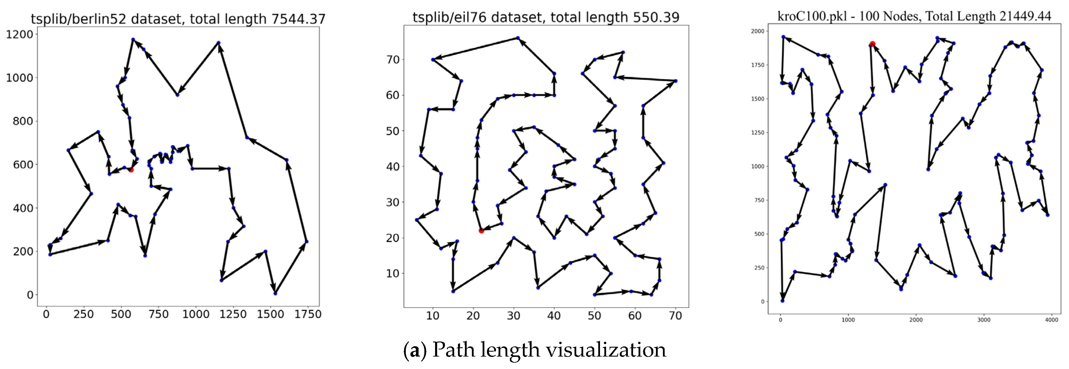
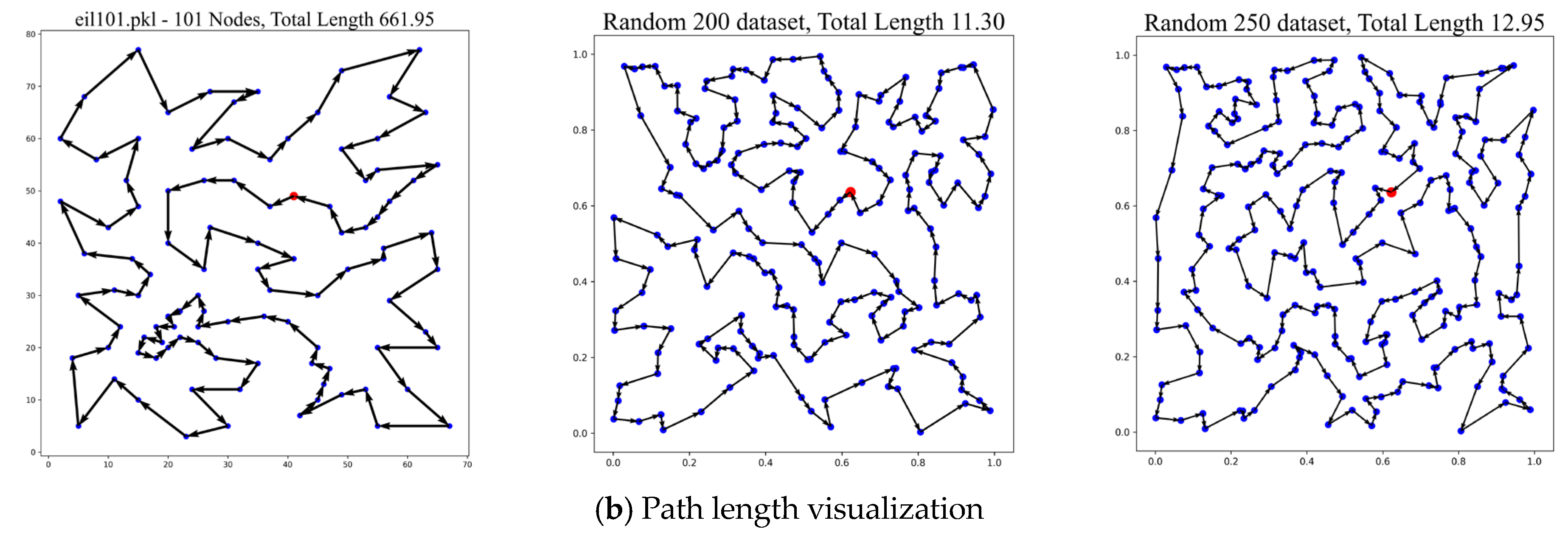
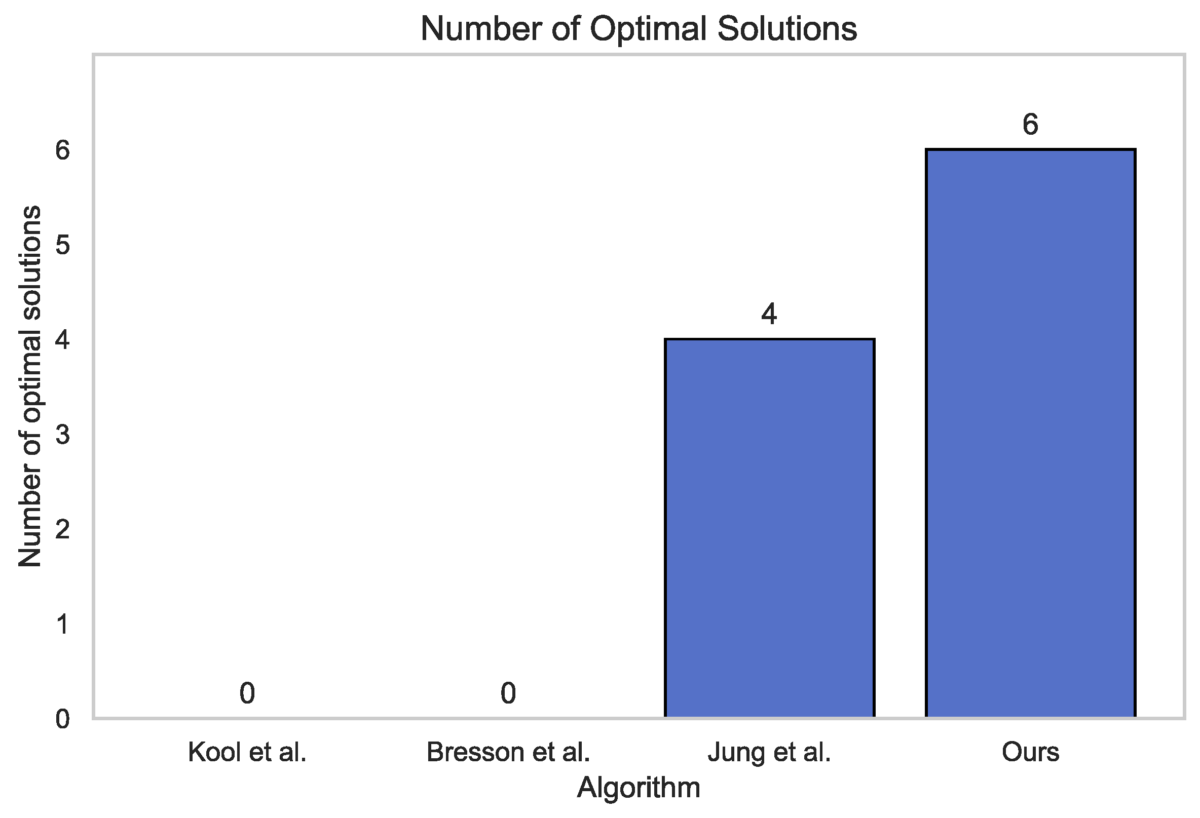
Figure 3 summarizes the comparative performance: our method secures optimal solutions for 6 out of 10 instances, while Kool’s and Bresson’s approaches yield no optimal solutions, and Jung’s method achieves 4. For small-scale instances, solution quality matches both Concorde’s exact solutions and Jung’s method, while large-scale instances exhibit significant improvements over all deep learning baselines, confirming robust generalization. Visualizations of representative tours are provided in Figure 4. Red markers denote starting cities, with blue markers indicating other cities. The algorithm iteratively constructs tours by sequentially visiting cities along arrow directions, ultimately returning to the origin. Visualization examples include varying problem scales and corresponding tour lengths.

To validate the statistical significance of the results, the Friedman test—a non-parametric statistical test suitable for comparing the performance rankings of multiple algorithms across multiple problem instances—was conducted on the four methods. The test revealed a statistically significant difference in performance among the methods across the 10 TSP instances (Friedman ${\chi }^2$ = 14.04, * p* < 0.01). As shown in

Table 4. Ranking Results by Different Methods.

Problem	Kool [25]	Bresson [14]	Jung [42]	Ours
eil51	4	3	1	2
berlin52	4	3	2	1
st70	3	4	1	2
eil76	2	4	3	1
kroA100	4	2	1	3
kroC100	3	4	2	1
rd100	4	2	1	3
eil101	2	4	3	1
ch130	2	4	3	1
ch150	3	4	2	1

, the proposed method achieved the best average rank (1.6), outperforming the baseline methods.

4.5. Ablation Experiment

To assess the contributions of the CTRGC and GAM, this study conducts ablation experiments on TSP100 using three model variants: Variant 1 (without CTRGC), Variant 2 (without GAM), and Variant 3 (lacking both components). As shown in

Table 5. Ablation experiments on key parts of the model.

Model	Len	Gap
Variant 1	7.817	0.73%
Variant 2	7.819	0.76%
Variant 3	7.821	0.78%
Ours	7.803	0.55%

and Figure 5, the full model achieves the smallest optimality gap, confirming that CTRGC’s dynamic relational matrices are critical for modeling local geometric dependencies, while GAM’s joint channel-spatial weighting effectively integrates global features. Both components independently improve performance compared to Variant 3, demonstrating their complementary roles in solution quality enhancement.

To further quantify the individual contributions of the CTRGC and GAM components to performance improvement, a contribution analysis was conducted based on ablation study results. The analysis revealed that CTRGC alone contributed a 0.02% performance gain, while GAM alone contributed 0.05%. Notably, their synergistic effect contributed 0.16%, indicating that the two components exhibit complementary functions, with synergy playing the dominant role in the overall improvement.

5. Discussion and Conclusions

This study has several limitations. First, the model’s performance on certain TSPLIB instances (e.g., rd100) still lags behind some baseline methods, indicating a need to enhance its adaptability to irregular node distributions. Second, although the linear attention mechanism reduces complexity, its scalability to very large-scale problems (e.g., TSP500+) has not been fully validated. Third, the current model is designed specifically for the Euclidean TSP; its generalization to variants with non-Euclidean or dynamically weighted distances requires further investigation.

The proposed Dynamic Topology-Aware Linear Attention Network (DTALAN) demonstrates superior performance in Traveling Salesman Problem (TSP) optimization through synergistic integration of local geometric modeling and global feature refinement. Experimental results reveal strong generalization across both synthetic and real-world benchmarks, with DTALAN achieving significantly smaller optimality gaps than traditional heuristics and state-of-the-art deep reinforcement learning methods. This validates two core innovations: (1) the Channel-aware Topology-Refined Graph Convolution (CTRGC), which dynamically captures local geometric dependencies, and (2) the Global Attention Mechanism (GAM), enabling effective cross-feature integration. Ablation studies confirm the indispensable role of CTRGC-GAM synergy—removing either component degrades solution quality. The decoder’s linear attention mechanism reduces computational complexity for large-scale problems, enabling efficient real-time path planning.

Our future work will extend the framework to broader combinatorial optimization domains, including vehicle routing (CVRP) and capacitated TSP variants. We will further validate robustness in non-Euclidean scenarios such as 3D logistics networks and multi-objective optimization systems.

References

1. Halim, A.H.; Ismail, I. Combinatorial Optimization: Comparison of Heuristic Algorithms in Travelling Salesman Problem. Arch. Comput. Methods Eng. 2017, 26, 367–380. [Google Scholar] [CrossRef]
2. Qian, W.-W.; Zhao, X.; Ji, K. Region Division in Logistics Distribution with a Two-Stage Optimization Algorithm. IEEE Access 2020, 8, 212876–212887. [Google Scholar] [CrossRef]
3. Onwubolu, G.C.; Clerc, M. Optimal path for automated drilling operations by a new heuristic approach using particle swarm optimization. Int. J. Prod. Res. 2004, 42, 473–491. [Google Scholar] [CrossRef]
4. Madani, A.; Batta, R.; Karwan, M. The balancing traveling salesman problem: Application to warehouse order picking. Top 2021, 29, 442–469. [Google Scholar] [CrossRef]
5. Sanyal, S.; Roy, K. Neuro-Ising: Accelerating Large-Scale Traveling Salesman Problems via Graph Neural Network Guided Localized Ising Solvers. IEEE Trans. Comput. Aided Des. Integr. Circuits Syst. 2022, 41, 5408–5420. [Google Scholar] [CrossRef]
6. Melab, N.; Mezmaz, M. Multi and many-core computing for parallel metaheuristics. Concurr. Comput. Pract. Exp. 2017, 29, e4116. [Google Scholar] [CrossRef]
7. Applegate, D.L.; Bixby, R.E.; Chvátal, V.; Cook, W.J. The Traveling Salesman Problem: A Computational Study. In The Traveling Salesman Problem; Princeton University Press: Princeton, NJ, USA, 2011. [Google Scholar]
8. Chen, P.; Wang, Q. Learning for multiple purposes: A Q-learning enhanced hybrid metaheuristic for parallel drone scheduling traveling salesman problem. Comput. Ind. Eng. 2024, 187, 109851. [Google Scholar] [CrossRef]
9. Helsgaun, K. An Extension of the Lin-Kernighan-Helsgaun TSP Solver for Constrained Traveling Salesman and Vehicle Routing Problems. Rosk. Rosk. Univ. 2017, 12, 966–980. [Google Scholar]
10. Wang, X.; Wang, S.; Liang, X.; Zhao, D.; Huang, J.; Xu, X.; Dai, B.; Miao, Q. Deep Reinforcement Learning: A Survey. IEEE Trans. Neural Netw. Learn. Syst. 2024, 35, 5064–5078. [Google Scholar] [CrossRef]
11. Ma, X.; Liu, C. A Travel Salesman Problem Solving Algorithm Based on Feature Enhanced Attention Model. J. Comput. 2024, 35, 215–230. [Google Scholar]
12. Liu, C.; Feng, X.-F.; Li, F.; Xian, Q.-L.; Jia, Z.-H.; Wang, Y.-H.; Du, Z.-D. Deep reinforcement learning combined with transformer to solve the traveling salesman problem. J. Supercomput. 2024, 81, 161. [Google Scholar] [CrossRef]
13. Vaswani, A.; Shazeer, N.M.; Parmar, N.; Uszkoreit, J.; Jones, L.; Gomez, A.N.; Kaiser, L.; Polosukhin, I. Attention is All you Need. In Proceedings of the Neural Information Processing Systems, Long Beach, CA, USA, 12 June 2017. [Google Scholar]
14. Bresson, X.; Laurent, T. The Transformer Network for the Traveling Salesman Problem. arXiv 2021. [Google Scholar] [CrossRef]
15. Okada, M.; Taji, K.; Fukushima, M. Probabilistic analysis of 2-opt for travelling salesman problems. Int. J. Syst. Sci. 1998, 29, 297–310. [Google Scholar] [CrossRef]
16. Christofides, N. Worst-Case Analysis of a New Heuristic for the Travelling Salesman Problem. Oper. Res. Forum 2022, 3, 20. [Google Scholar] [CrossRef]
17. Clarke, G.; Wright, J.W. Scheduling of Vehicles from a Central Depot to a Number of Delivery Points. Oper. Res. 1964, 12, 568–581. [Google Scholar] [CrossRef]
18. Bellmore, M.; Nemhauser, G.L. The Traveling Salesman Problem: A Survey. Oper. Res. 1968, 16, 538–558. [Google Scholar] [CrossRef]
19. Rosenkrantz, D.J.; Stearns, R.E.; Lewis, P.M., II. An Analysis of Several Heuristics for the Traveling Salesman Problem. SIAM J. Comput. 1977, 6, 563–581. [Google Scholar] [CrossRef]
20. Sui, J.; Ding, S.; Huang, X.; Yu, Y.; Liu, R.; Xia, B.; Ding, Z.; Xu, L.; Zhang, H.; Yu, C.; et al. A survey on deep learning-based algorithms for the traveling salesman problem. Front. Comput. Sci. 2024, 19, 196322. [Google Scholar] [CrossRef]
21. Vinyals, O.; Fortunato, M.; Jaitly, N. Pointer Networks. arXiv 2015. [Google Scholar] [CrossRef]
22. Bello, I.; Pham, H.; Le, Q.V.; Norouzi, M.; Bengio, S. Neural Combinatorial Optimization with Reinforcement Learning. arXiv 2017. [Google Scholar] [CrossRef]
23. Nazari, M.; Oroojlooy, A.; Snyder, L.; Takác, M. Reinforcement Learning for Solving the Vehicle Routing Problem. In Proceedings of the Neural Information Processing Systems, Montréal, QC, Canada, 12 February 2018. [Google Scholar]
24. Deudon, M.; Cournut, P.; Lacoste, A.; Adulyasak, Y.; Rousseau, L.-M. Learning Heuristics for the TSP by Policy Gradient. In Integration of Constraint Programming, Artificial Intelligence, and Operations Research; Van Hoeve, W.-J., Ed.; Springer International Publishing: Cham, Switzerland, 2018; pp. 170–181. [Google Scholar]
25. Kool, W.; Hoof, H.V.; Welling, M. Attention, Learn to Solve Routing Problems! In Proceedings of the International Conference on Learning Representations, Vancouver, BC, Canada, 22 March 2018. [Google Scholar]
26. Kwon, Y.-D.; Choo, J.; Kim, B.; Yoon, I.; Gwon, Y.; Min, S. POMO: Policy Optimization with Multiple Optima for Reinforcement Learning. In Proceedings of the Advances in Neural Information Processing Systems 33 (NeurIPS 2020), Virtual, 30 October 2020. [Google Scholar]
27. Pan, X.; Jin, Y.; Ding, Y.; Feng, M.; Zhao, L.; Song, L.; Bian, J. H-TSP: Hierarchically Solving the Large-Scale Travelling Salesman Problem. In Proceedings of the AAAI Conference on Artificial Intelligence (AAAI 2023), Washington, DC, USA, 7–14 February 2023. [Google Scholar]
28. Lischka, A.; Wu, J.; Basso, R.; Chehreghani, M.H.; Kulcsár, B. Less is More—On the Importance of Sparsification for Transformers and Graph Neural Networks for TSP. arXiv 2024, arXiv:2403.17159. [Google Scholar]
29. Luo, F.; Lin, X.; Liu, F.; Zhang, Q.; Wang, Z. Neural Combinatorial Optimization with Heavy Decoder: Toward Large Scale Generalization. In Proceedings of the Neural Information Processing Systems (NeurIPS) 2023, Main Conference Track, New Orleans, LA, USA, 10 December 2023. [Google Scholar]
30. Khalil, E.B.; Dai, H.; Zhang, Y.; Dilkina, B.; Song, L. Learning Combinatorial Optimization Algorithms over Graphs. arXiv 2017, arXiv:1704.01665. [Google Scholar]
31. Ma, Q.; Ge, S.; He, D.; Thaker, D.; Drori, I. Combinatorial Optimization by Graph Pointer Networks and Hierarchical Reinforcement Learning. arXiv 2019, arXiv:1911.04936. [Google Scholar]
32. Drori, I.; Kharkar, A.; Sickinger, W.R.; Kates, B.; Ma, Q.; Ge, S.; Dolev, E.; Dietrich, B.; Williamson, D.P.; Udell, M. Learning to Solve Combinatorial Optimization Problems on Real-World Graphs in Linear Time. In Proceedings of the 2020 19th IEEE International Conference on Machine Learning and Applications (ICMLA), Miami, FL, USA, 14–17 December 2020; pp. 19–24. [Google Scholar]
33. Lei, K.; Guo, P.; Wang, Y.; Wu, X.; Zhao, W. Solve routing problems with a residual edge-graph attention neural network. Neurocomputing 2022, 508, 79–98. [Google Scholar] [CrossRef]
34. Ouyang, W.; Wang, Y.; Weng, P.; Han, S. Generalization in Deep RL for TSP Problems via Equivariance and Local Search. arXiv 2021, arXiv:2110.03595. [Google Scholar]
35. Chen, Y.; Zhang, Z.; Yuan, C.; Li, B.; Deng, Y.; Hu, W. Channel-wise Topology Refinement Graph Convolution for Skeleton-Based Action Recognition. arXiv 2021, arXiv:2110.03595. [Google Scholar]
36. Liu, Y.; Shao, Z.; Hoffmann, N. Global Attention Mechanism: Retain Information to Enhance Channel-Spatial Interactions. arXiv 2021, arXiv:2112.05561. [Google Scholar]
37. Beltagy, I.; Peters, M.E.; Cohan, A. Longformer: The Long-Document Transformer. arXiv 2020. [Google Scholar] [CrossRef]
38. Kingma, D.P.; Ba, J. Adam: A Method for Stochastic Optimization. arXiv 2017. [Google Scholar] [CrossRef]
39. Reinelt, G. TSPLIB—A Traveling Salesman Problem Library. ORSA J. Comput. 1991, 3, 376–384. [Google Scholar] [CrossRef]
40. Xu, Y.; Fang, M.; Chen, L.; Xu, G.; Du, Y.; Zhang, C. Reinforcement Learning with Multiple Relational Attention for Solving Vehicle Routing Problems. IEEE Trans. Cybern. 2022, 52, 11107–11120. [Google Scholar] [CrossRef]
41. Joshi, C.K.; Cappart, Q.; Rousseau, L.-M.; Laurent, T. Learning TSP Requires Rethinking Generalization. In Proceedings of the 27th International Conference on Principles and Practice of Constraint Programming (CP 2021), Montpellier, France, 25–29 October 2021; Volume 2021, pp. 33:1–33:21. [Google Scholar]
42. Jung, M.; Lee, J.; Kim, J. A lightweight CNN-transformer model for learning traveling salesman problems. Appl. Intell. 2024, 54, 7982–7993. [Google Scholar] [CrossRef]
43. Zhang, R.; Prokhorchuk, A.; Dauwels, J. Deep Reinforcement Learning for Traveling Salesman Problem with Time Windows and Rejections. In Proceedings of the 2020 International Joint Conference on Neural Networks (IJCNN), Glasgow, UK, 19–24 July 2020; pp. 1–8. [Google Scholar]
Figure 1. Structure of the model.
Mathematics 14 00166 g001
Figure 2. Structure of encoder and decoder.
Mathematics 14 00166 g002
Figure 3. The number of optimal solutions obtained by each algorithm [14,25,42].
Mathematics 14 00166 g003
Figure 4. Path length visualization. (The red dots represent the starting city, while the blue dots represent the other cities).
Mathematics 14 00166 g004aMathematics 14 00166 g004b
Figure 5. Model training convergence plot.
Mathematics 14 00166 g005