Article

EpilepsyNet-XAI: Towards High-Performance and Explainable Multi-Phase Seizure Analysis from EEG Features

1
Department of Creative Technologies, Air University, Islamabad 44000, Pakistan
2
Department of AI and Software, Gachon University, Seongnam-si 13120, Gyeonggi-do, Republic of Korea
3
Medical Device Development Center, Osong Medical Innovation Foundation, Cheongju 28160, Chungbuk, Republic of Korea
*
Authors to whom correspondence should be addressed.
Mathematics 2026, 14(1), 125; https://doi.org/10.3390/math14010125 (registering DOI)
Submission received: 6 November 2025 / Revised: 19 December 2025 / Accepted: 24 December 2025 / Published: 29 December 2025
(This article belongs to the Special Issue Methods, Analysis and Applications in Computational Neuroscience)

Abstract

Epilepsy is a long-term neurological disorder affecting more than 65 million people worldwide, and accurate detection of its phases from electroencephalogram (EEG) signals is essential for diagnosis and patient management. This paper presents a comprehensive method for multi-phase seizure classification using robust feature engineering, advanced machine learning (ML), deep learning (DL), and explainable artificial intelligence (XAI). A rich set of EEG features is constructed, combining traditional and specialized metrics to capture subtle neurophysiological shifts across seizure phases. Exploratory data analysis demonstrates the discriminative power of these features, with PCA and t-SNE revealing distinct non-linear clusters. Multiple ML models—including Random Forest, Support Vector Machines, K-Nearest Neighbors, LightGBM, and XGBoost—are evaluated using 5-fold stratified cross-validation, achieving consistently high performance. The proposed MLP-based EpilepsyNet-XAI model outperforms all baselines. Post hoc XAI techniques such as LIME are applied to enhance transparency and interpretability in the classification process. By integrating high-performing models with interpretable analysis, this work supports more reliable AI-driven approaches for methodological epilepsy research and analysis.

1. Introduction

Epilepsy is one of the most common chronic neurological disorders of the brain, characterized by recurrent seizures caused by abnormal neuronal activity [1]. A seizure results from sudden bursts of electrical discharges among brain cells, affecting muscle control, sensations, emotions, and behavior [2]. In the United States alone, approximately 3.4 million people live with epilepsy, including 3 million adults and 470,000 children, while globally, more than 65 million individuals are affected [3]. According to the 2023 WHO report, epilepsy involves unprovoked seizures arising from abnormal synchronous neuronal firing in the brain [4,5]. These episodes can significantly impair cognitive function, physical safety, and quality of life, underscoring the importance of accurate and timely seizure detection for effective diagnosis, treatment, and management.
Electroencephalography (EEG) remains the primary technique for monitoring electrical brain activity and identifying epileptic abnormalities [6]. However, manual EEG interpretation by neurologists is labor-intensive, time-consuming, and prone to subjective variability, potentially delaying intervention and increasing the risk of misdiagnosis [7]. Although automated systems have been developed, most focus only on binary seizure detection—seizure vs. non-seizure—thereby overlooking the transitional dynamics across the continuum of normal, pre-seizure, seizure, and post-seizure phases [8,9,10]. Pre-seizure detection, in particular, is clinically crucial because early-warning capability enables preventive actions or therapeutic interventions before seizure onset [11]. Furthermore, accurate post-seizure characterization provides insights into recovery patterns and post-ictal complications [12].
Machine learning (ML) and deep learning (DL) techniques have shown strong potential for early epilepsy detection by learning complex patterns from high-dimensional EEG representations [13,14]. Despite their performance advantages, many ML/DL models function as “black boxes,” offering limited interpretability and restricting clinical trust [15]. Clinicians require not only accurate predictions but also transparent explanations of how models arrive at those predictions.
To address these gaps, we propose a comprehensive, interpretable framework for multi-class EEG state classification using a wide range of EEG-derived features. The feature space includes time-domain, frequency-domain, wavelet-based, nonlinear dynamic, and event-related EEG descriptors extracted from a large clinical EEG dataset. These diverse features capture subtle statistical, spectral, and complexity-based patterns associated with different labeled EEG states. Additionally, visualization and dimensionality reduction techniques—including topographic mapping, Principal Component Analysis (PCA), and t-distributed Stochastic Neighbor Embedding (t-SNE)—are employed to examine feature distribution and class separability.
Multiple ML models—including Random Forest (RF), Support Vector Machine (SVM), K-Nearest Neighbors (KNN), LightGBM, and XGBoost—are compared against a custom deep learning model, EpilepsyNet-XAI, designed for multi-class classification across all four seizure phases. To ensure transparency, Explainable AI (XAI) techniques, specifically SHAP and LIME, are integrated to provide global and local interpretability, enabling clinicians to understand the underlying biomarkers driving each model decision [16,17].

Objectives and Contributions

This study aims to develop a transparent and empirically rigorous framework for epileptic seizure detection through supervised classification of EEG signal segments using classical machine learning techniques applied to publicly available EEG datasets. While deep learning approaches dominate recent literature, classical supervised models remain attractive due to their interpretability, lower computational requirements, and suitability for clinical integration. However, prior studies on public EEG datasets rarely provide systematic evaluation across feature groups, robustness testing, or model-agnostic interpretability.
To address these gaps, our contributions are summarized as follows:
  • Comprehensive feature-engineering pipeline: We extract and organize a structured set of time-domain, frequency-domain, and entropy-based features validated in neuroscientific and biomedical signal-processing literature. We explicitly evaluate the discriminative power of each feature group to ensure transparency and reproducibility.
  • Systematic benchmarking of classical supervised models: Five widely adopted classifiers—Random Forest, Support Vector Machine, k-Nearest Neighbors, Gradient Boosting, and Multilayer Perceptron—are trained and compared under consistent preprocessing, segmentation, and class-balancing procedures.
  • Model-agnostic interpretability using SHAP and LIME: We integrate SHAP and LIME explainability tools to quantify the contribution of individual EEG-derived features, providing clinically relevant interpretation that is often missing in prior public-dataset EEG studies.
  • Ablation and robustness analyses: We introduce systematic evaluations, including feature-group ablation, class imbalance robustness, and noise perturbation analysis, thereby strengthening the empirical depth and distinguishing the work from prior studies.
  • Reproducible workflow: The proposed pipeline is modular and easy to reproduce, enabling future extensions with alternative feature sets or hybrid models.
As illustrated in Figure 1, the proposed EpilepsyNet-XAI framework forms a complete pipeline for multi-phase seizure detection and interpretability. It begins with the EEG dataset, followed by extraction of diverse time, spectral, wavelet-based, and nonlinear features that characterize seizure-related brain dynamics. These features are used to train and evaluate multiple ML models under a stratified cross-validation strategy, where the proposed EpilepsyNet-XAI demonstrates superior accuracy and stability. Finally, XAI methods are employed to analyze feature importance and local decision rationale, providing clinically interpretable explanations of the neural biomarkers associated with each seizure phase.
The remainder of this paper is structured as follows: Section 2 details the EEG dataset and feature extraction methodology, and describes the architectural design of EpilepsyNet-XAI and the baseline ML models. Section 3 presents the experimental results, including performance metrics and a detailed interpretability analysis. Section 3 concludes the paper with key findings and future research directions.

2. Materials and Methods

This section presents the dataset, feature engineering process, model development, cross-validation strategy, and performance evaluation metrics employed in the proposed study.

2.1. Dataset

This study employs the publicly available Epilepsy Detection Dataset hosted on Kaggle, derived from real clinical EEG recordings originally collected in a hospital setting and subsequently released in fully anonymized form for research use. The public version contains only pre-extracted segment-level features and labels; raw EEG waveforms, subject identifiers, and session-level metadata are not included to ensure privacy protection. According to the original repository documentation, the data were sampled at 256 Hz using a multi-channel clinical EEG system, and all recordings underwent de-identification prior to release in compliance with institutional ethics approvals.
The Kaggle version represents a feature-level reconstruction of these clinical signals, providing 289,010 EEG segments together with engineered statistical, spectral, wavelet, and nonlinear descriptors, along with basic demographic metadata (age, gender, medication status, and seizure history). All features are computed independently for each EEG segment using only the signal samples contained within that segment, without access to seizure onset or offset annotations, seizure boundaries, or future temporal context. As subject-level identifiers are unavailable, model training and evaluation rely on segment-level stratified cross-validation; this limitation and its implications for generalizability are discussed in Section 4.
Table 1 summarizes the structure of the dataset. Because subject identifiers are not available in the public release, segment-level stratified cross-validation is employed.

2.2. Data Preprocessing and Exploratory Analysis

We performed systematic data preprocessing to prepare the engineered EEG features for robust model training and to mitigate issues such as varying scales, missing values, skewness, and outliers. Preprocessing steps included data cleaning (removal of corrupted records), imputation of missing values using median imputation for numerical features, and feature scaling. For scaling we used robust approaches (e.g., RobustScaler or standardization) depending on the presence of outliers; any transformation (scaler, log or Yeo–Johnson) was fitted only on training data within each cross-validation fold to avoid data leakage.
Dimensionality reduction and visualization techniques, including Principal Component Analysis (PCA) and t-Distributed Stochastic Neighbor Embedding (t-SNE), were applied to explore the structure of the feature space and to assess separability across seizure phases. Additionally, we examined single-feature distributions and channel-level interactions (e.g., cross-correlation between EEG channels) to identify biomarkers and to inform subsequent feature selection.
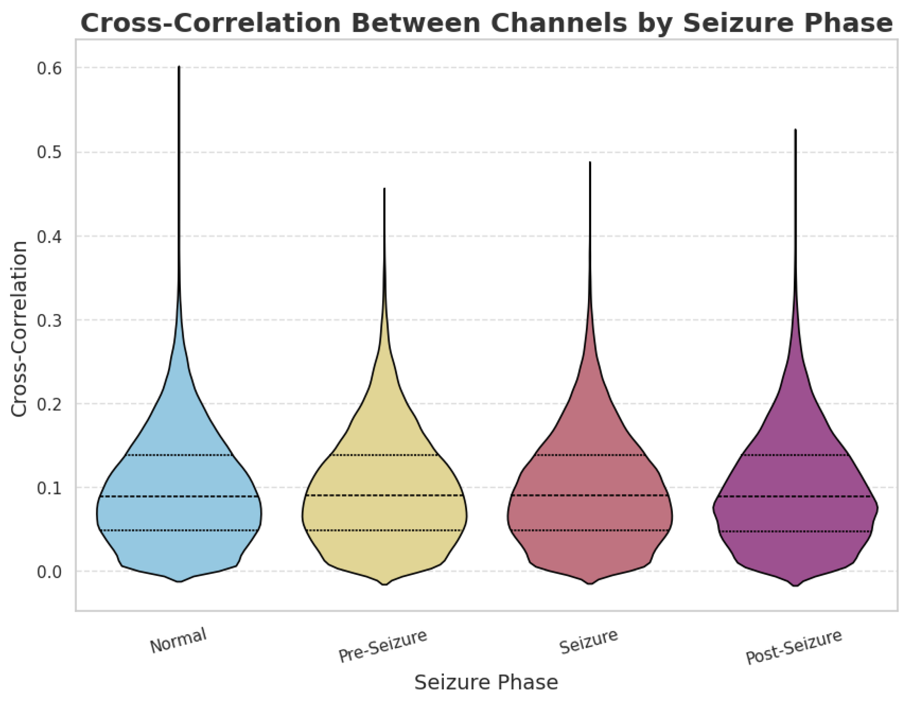
Figure 2 displays the distribution of the Cross_Correlation_Between_Channels feature across the four seizure phases. The Normal phase exhibits a slightly wider distribution compared with the other phases, indicating greater variability in inter-channel correlation during non-ictal periods. Median values across phases are broadly comparable, suggesting that while central tendency may be similar, the dispersion and tails differ—information that can be useful for feature selection and modeling. These exploratory findings motivated the inclusion of connectivity-based and dispersion-sensitive features in the final feature set.
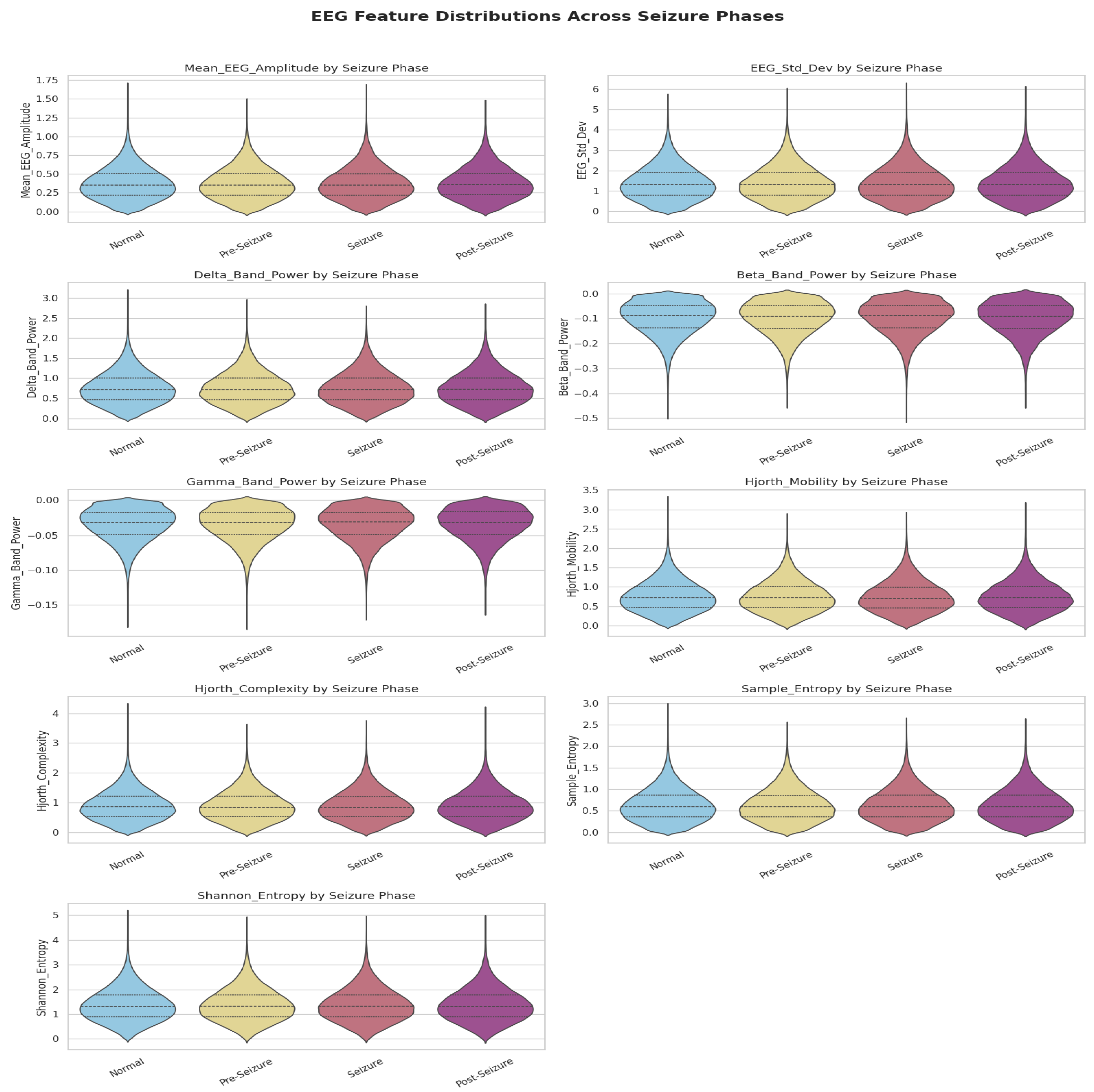
Figure 3 illustrates how advanced non-linear and wavelet-derived EEG features vary across distinct seizure states. These metrics—such as permutation entropy, Lyapunov exponent, Hurst exponent, Higuchi fractal dimension, Lempel–Ziv complexity, wavelet entropy, and wavelet energy—demonstrate characteristic shifts that enhance the separability between phases. Such discriminative features effectively capture the intrinsic signal complexity and temporal dynamics of brain activity, thereby improving the differentiation of normal, pre-seizure, seizure, and post-seizure conditions.
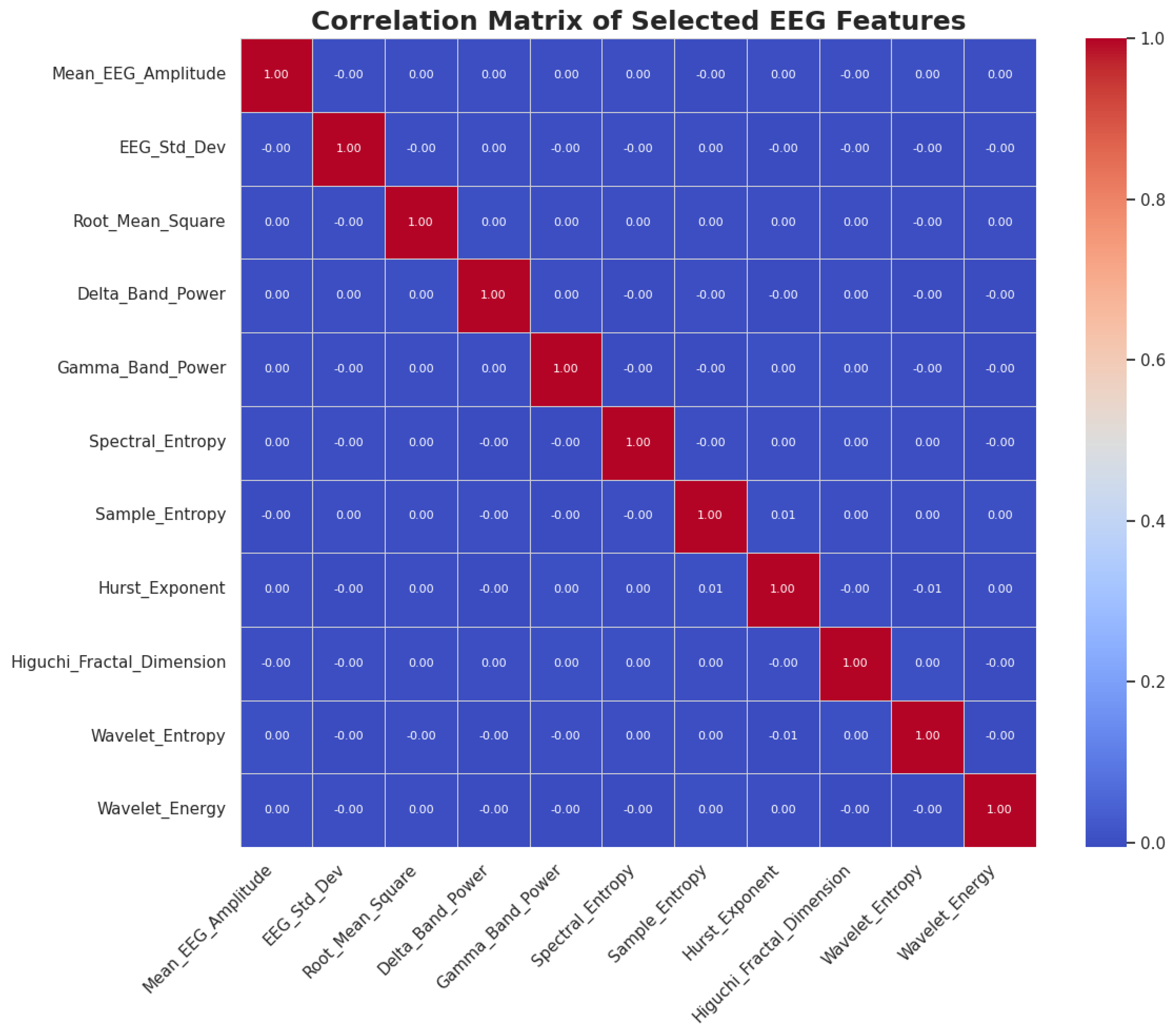
Figure 4 illustrates the correlation matrix of selected EEG features, highlighting the pairwise relationships among both linear and non-linear measures. The near-zero correlation values across most feature pairs indicate minimal redundancy, suggesting that each feature contributes unique information to the characterization of EEG signals. This low inter-feature dependence supports the effectiveness of combining diverse statistical, spectral, and entropy-based descriptors for improved seizure phase discrimination.

2.2.1. Feature Engineering

The dataset includes 52 pre-extracted EEG features, systematically categorized to capture spectral, statistical, nonlinear, and connectivity characteristics relevant to segment-level EEG characterization for multi-class classification. After preprocessing, the RobustScaler was applied to reduce the influence of outliers and stabilize feature distributions. To maintain the natural class distribution, no data augmentation or oversampling techniques were applied; instead, stratified splitting was used to balance class proportions across folds. Rather than relying on manual feature selection, we employed a Random Forest (RF)-based importance ranking combined with correlation filtering to identify the most informative subset of features for classical ML models. As a result, 23 features were selected for ML-based classification.
All features used in this study are computed independently at the level of individual EEG segments and are derived solely from the signal samples contained within each segment. No information regarding seizure onset, offset, seizure phase labels, or future temporal context is used during feature computation. Features that may appear seizure-related in name (e.g., seizure intensity index or spike rate) are implemented as generic signal descriptors based on amplitude, frequency, or transient detection thresholds applied uniformly to all segments, regardless of class. This design ensures a label-agnostic, causal feature extraction process and eliminates the possibility of label leakage.
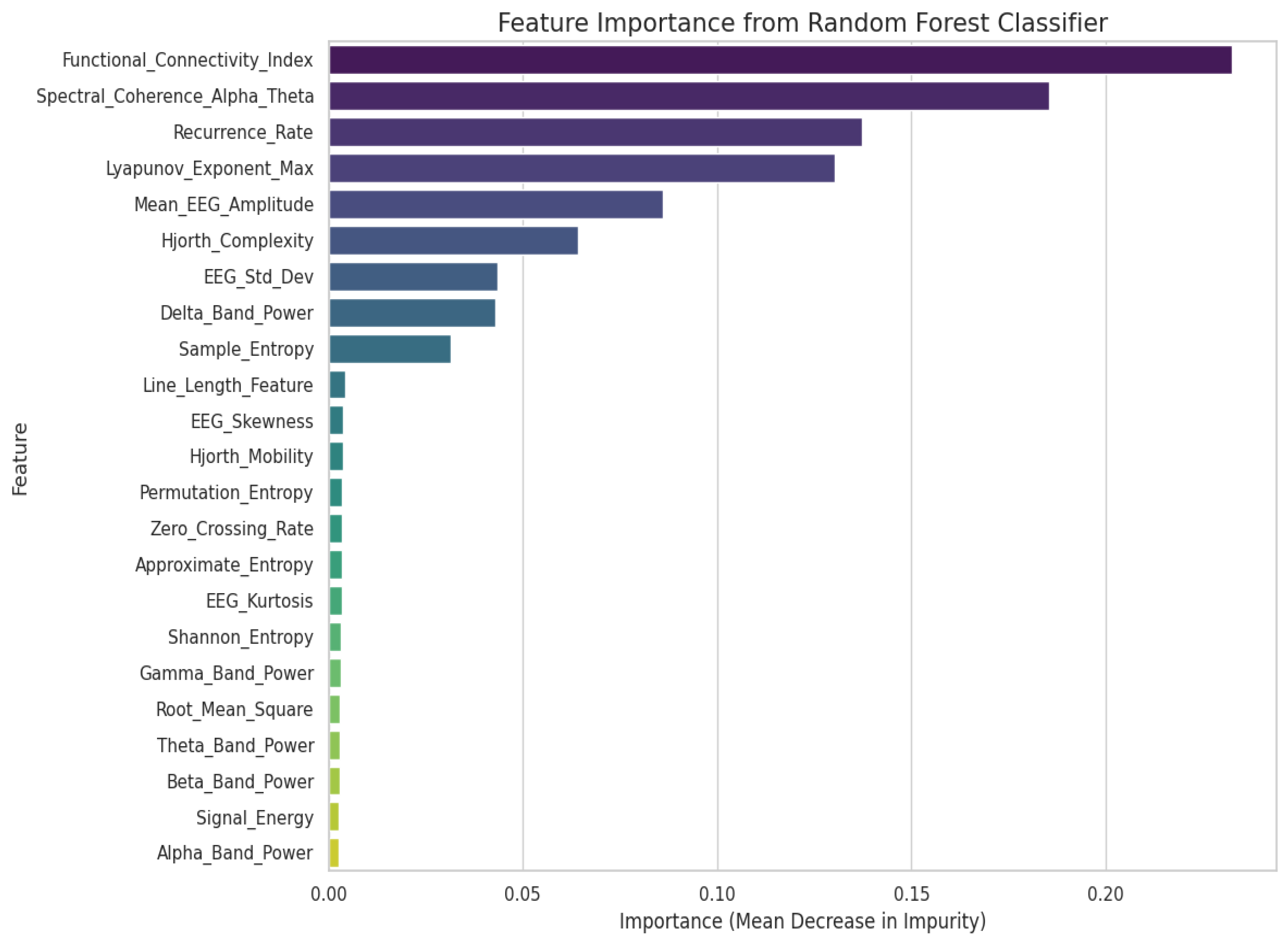
Figure 5 highlights that both original and newly introduced specialized features are among the most discriminative EEG biomarkers. The dominance of features such as FCI, RR, LEM, and SCAT validates their significance in capturing subtle EEG dynamics that differ across normal, pre-seizure, and post-seizure conditions. For instance, elevated Δ -band power or mean EEG amplitude typically reflects heightened neural activity observed during seizure segments, while higher entropy measures suggest distinct brain state dynamics. The feature importance analysis derived from the RF model thus provides a data-driven understanding of EEG patterns that support reliable discrimination among the annotated seizure-related states, offering valuable insights for both model optimization and neurophysiological interpretation.
The variations in EEG feature patterns across different annotated seizure-related states are visualized through normalized profiles. As illustrated in Figure 6, these radial plots—conceptualized as feature topographic maps—demonstrate distinct signatures of mean EEG amplitude, band power, and complexity measures across normal, pre-seizure, seizure, and post-seizure segments. The prominent shifts observed in these multi-feature patterns across labeled states provide strong evidence of their discriminative potential, forming the basis for robust multi-class EEG segment classification.
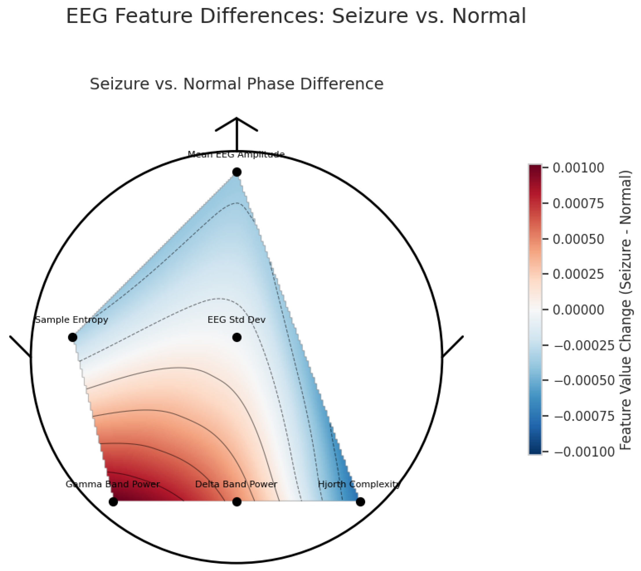
Differences between normal and ictal EEG segments provide a quantitative representation of changes in brain dynamics associated with seizure activity. As illustrated in Figure 7, distinct EEG features exhibit notable variations between segments labeled as normal and seizure. Specifically, δ Band Power, Γ Band Power, and Hjorth Complexity demonstrate significant positive shifts, reflecting increased neural activity and signal complexity in seizure segments. Conversely, Sample Entropy tends to decrease, indicating a reduction in signal regularity. These complementary trends collectively characterize the pronounced divergence of EEG dynamics between normal and seizure-labeled segments.
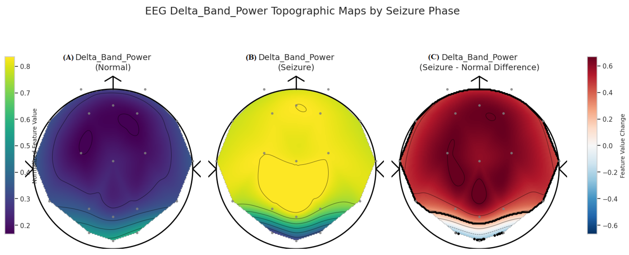
Topographic maps are generated for key EEG features to visualise the spatial distribution and dynamic changes in brain activity captured by these features. As shown in Figure 8, the distribution of δ -band power differs markedly between normal EEG segments and seizure-labeled EEG segments. A substantial increase in δ -band power is observed in seizure segments, indicating heightened cortical synchronisation and distinct spatial patterns associated with ictal activity.
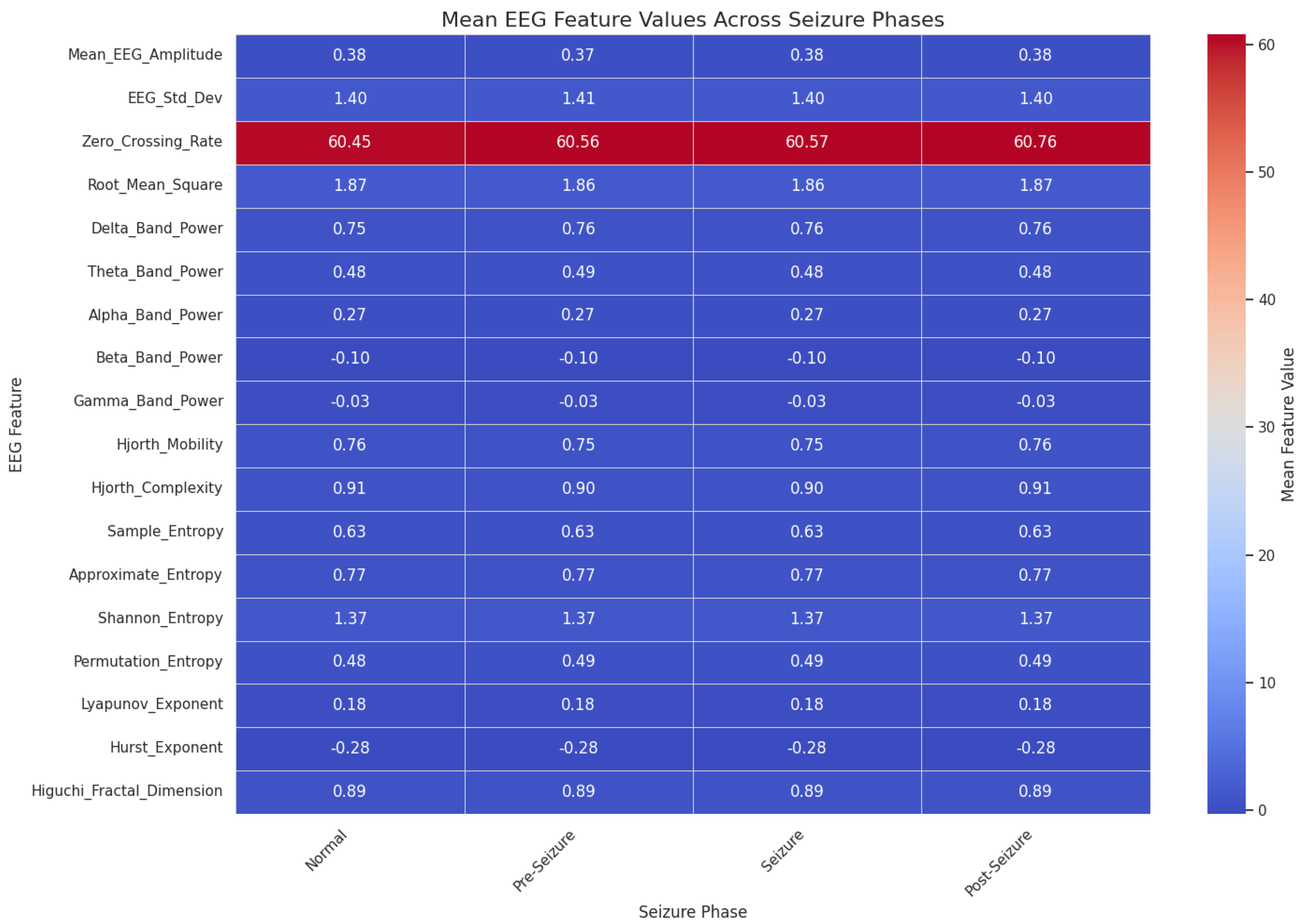
The zero-crossing rate exhibits a noticeable increase in EEG segments labeled as seizure, indicating heightened signal variability. To further explore the discriminative capacity of the engineered features, Figure 9 illustrates the mean values of a broad range of EEG features across the four labeled EEG states—normal, pre-seizure, seizure, and post-seizure. Each label exhibits a distinct average feature profile, reflecting the unique neurophysiological dynamics associated with that class. These patterns provide strong evidence of the engineered features’ ability to differentiate among labeled EEG states and highlight their relevance for accurate multi-class seizure classification.
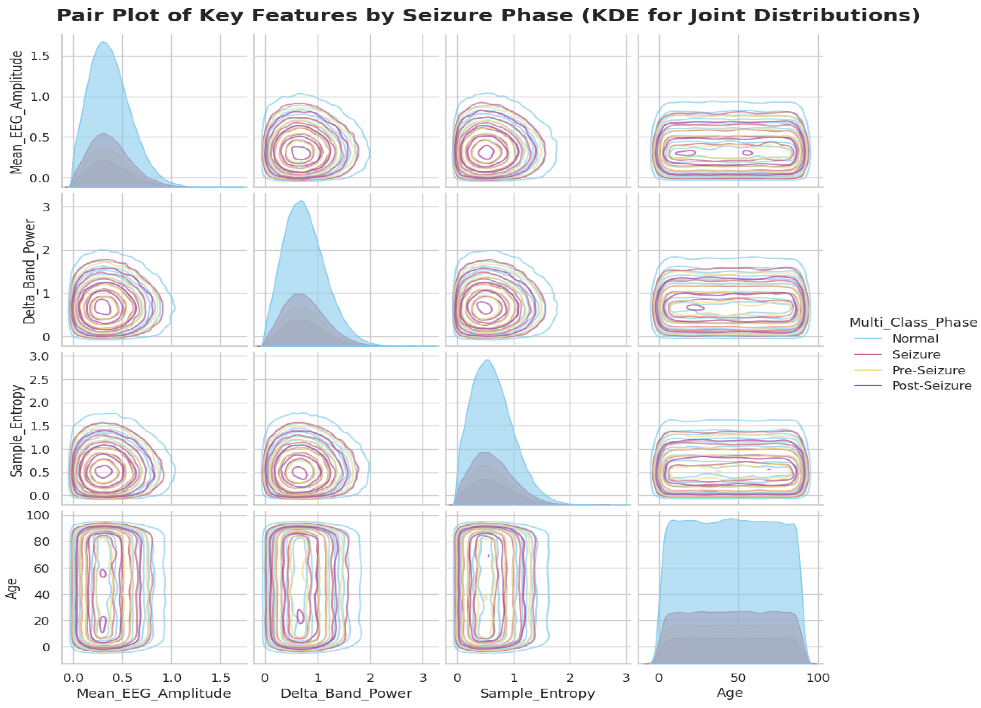
The multivariate relationships among key EEG features were further explored through pair plots employing Kernel Density Estimates (KDEs), as shown in Figure 10. The diagonal subplots depict the univariate distributions of mean EEG amplitude, δ -band power, sample entropy, and age across different labeled EEG states, while the off-diagonal subplots illustrate their bivariate joint distributions. This visualization clearly reveals that features such as δ -band power exhibit strong class separability between the Normal, Pre-Seizure, Seizure, and Post-Seizure classes. In contrast, the age feature shows expected overlap across all labels, serving as a non-discriminative demographic context variable. Overall, the pair-plot analysis highlights the multivariate structure of the dataset and underscores the discriminative strength of the engineered EEG features for robust multi-class classification.
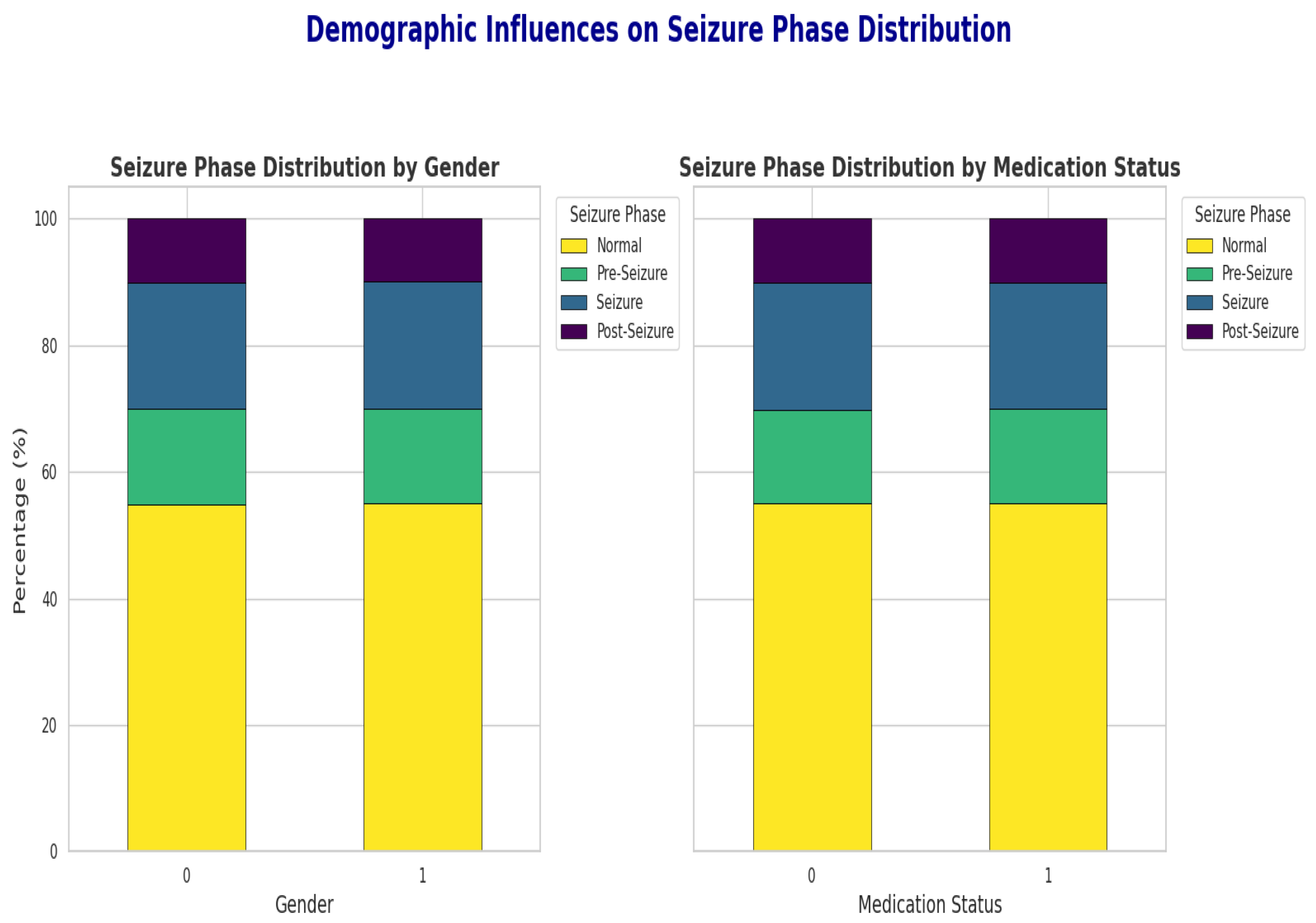
Gender and medication factors were further examined to assess their influence on the distribution of labeled EEG states. As illustrated in Figure 11, the proportional representation of each class (Normal, Pre-Seizure, Seizure, and Post-Seizure) remains largely consistent across different gender groups and medication statuses. This observation indicates that demographic factors such as gender and medication use do not introduce noticeable bias into the dataset, thereby supporting the robustness and generalizability of the developed model.
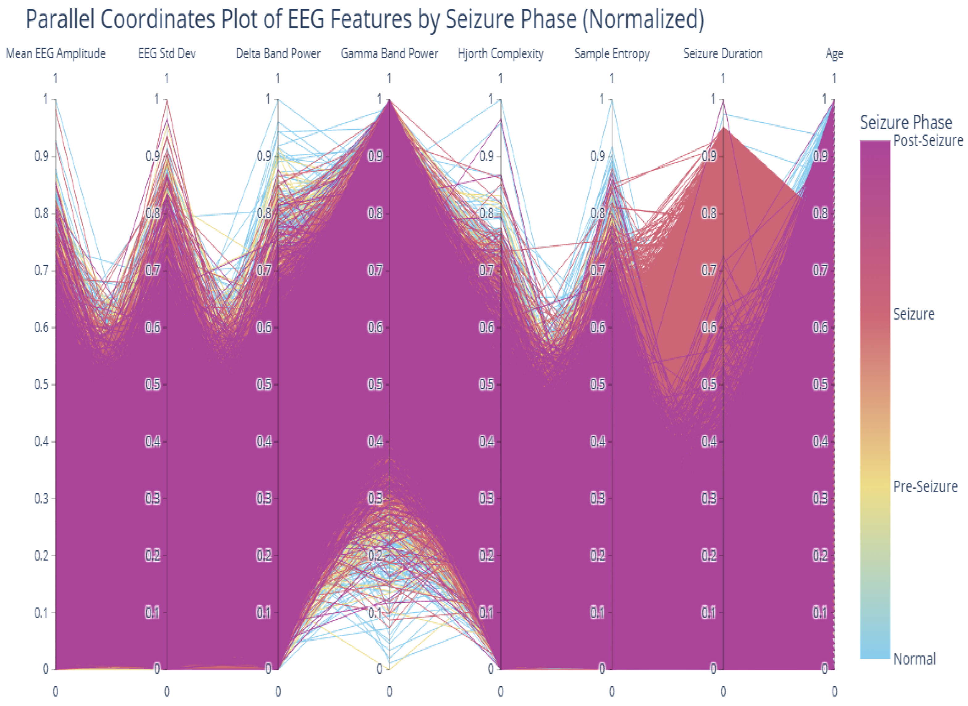
Multi-dimensional feature trajectories visualized through parallel coordinates are shown in Figure 12. Each vertical axis represents a specific normalized EEG feature, while the colored lines correspond to individual data samples across different labeled EEG states. The clustering and divergence patterns observed along these axes reveal distinct multi-feature fingerprints for each class. These trajectories highlight the high discriminative potential of the engineered features and provide deeper insights into the complex physiological patterns underlying epileptic EEG activity.

2.2.2. Dimensionality Reduction

To visualize and interpret the separability of EEG features across different seizure phases, we employ two complementary dimensionality reduction techniques: Principal Component Analysis (PCA) and t-Distributed Stochastic Neighbor Embedding (t-SNE). These techniques project the high-dimensional feature vectors into two-dimensional subspaces, facilitating intuitive analysis of class distributions and feature discriminability.
PCA is a linear transformation method that projects data onto orthogonal axes of maximum variance. It is derived from the eigenvalue decomposition of the covariance matrix of the feature data. Let X denote the feature matrix and Σ its covariance matrix. The principal components are the eigenvectors (v) of Σ , and the proportion of variance explained by each component corresponds to its eigenvalue ( λ ), as defined in Equation (1).
Σ v = λ v
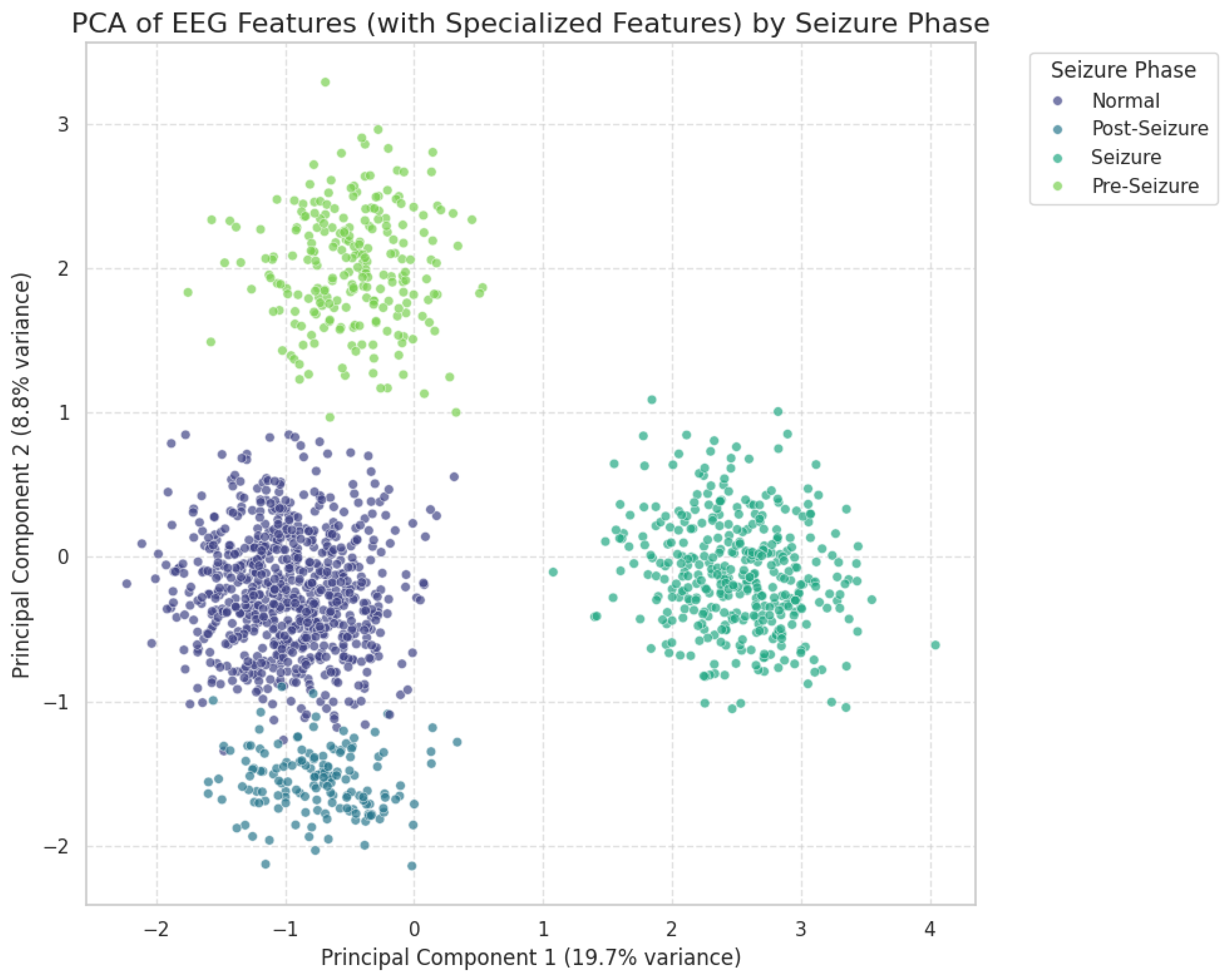
We select the top k eigenvectors corresponding to the largest eigenvalues to project the high-dimensional EEG data onto a lower k-dimensional subspace (two dimensions in our case), thereby retaining most of the original variance. The PCA visualization in Figure 13 illustrates that the specialized feature set enhances clustering and linear separability among seizure phases, including pre-seizure, seizure, post-seizure, and normal states.
While PCA effectively captures global linear variance, it may fail to preserve nonlinear relationships inherent in EEG data. To address this, we employ t-Distributed Stochastic Neighbor Embedding (t-SNE), a nonlinear dimensionality reduction technique that models pairwise similarities between data points in both high- and low-dimensional spaces. By minimizing the Kullback–Leibler divergence between these similarity distributions, t-SNE preserves local neighborhood structures and reveals nonlinear cluster formations.
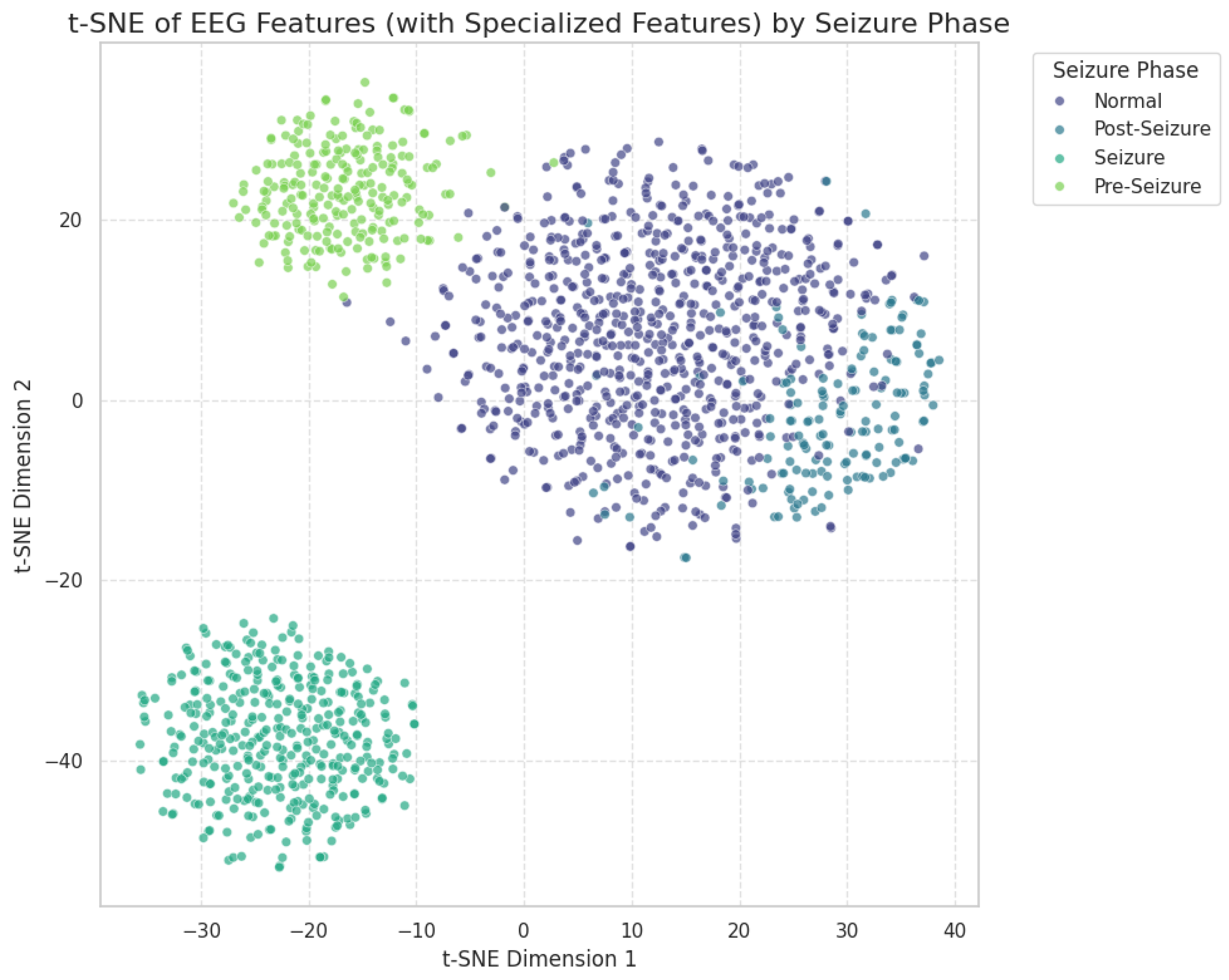
As shown in Figure 14, t-SNE produces distinct and well-separated clusters corresponding to different seizure phases. The specialized features enhance this nonlinear separability, indicating that the proposed feature engineering strategy captures phase-specific EEG characteristics more effectively than conventional approaches. Together, the PCA and t-SNE visualizations confirm that the extracted features encode discriminative patterns essential for robust multi-phase seizure detection.
t-SNE constructs a probability distribution that represents the pairwise similarity between data points x i and x j in the original high-dimensional EEG feature space. The conditional probability p j | i reflects the likelihood that x j would be selected as a neighbor of x i , assuming a Gaussian distribution centered at x i , as defined in Equation (2).
p j | i = exp x i x j 2 2 σ i 2 k i exp x i x k 2 2 σ i 2
In this formulation, nearby points in the high-dimensional space have higher probabilities of being neighbors. The bandwidth parameter σ i is chosen individually for each data point based on a predefined perplexity, which determines the effective number of neighbors considered.
To obtain a symmetric joint probability distribution, the conditional probabilities are combined as follows:
p i j = p j | i + p i | j 2 N
In our study, the EEG feature dataset consists of 52 engineered features in total, including 48 quantitative EEG signal descriptors and 4 demographic metadata variables, resulting in a 52-dimensional feature space. The probability distribution p i j , defined in Equation (3), captures the intrinsic similarity relationships among data points within this complex, high-dimensional space.
To map the data into a lower-dimensional space, t-SNE defines a similar probability distribution q i j over the low-dimensional embeddings y i and y j using a Student’s t-distribution with one degree of freedom, as shown in Equation (4).
q i j = ( 1 + y i y j 2 ) 1 k l ( 1 + y k y l 2 ) 1
The objective of t-SNE is to minimize the divergence between the high-dimensional similarity distribution p i j and its low-dimensional counterpart q i j . This is achieved by minimizing the Kullback–Leibler (KL) divergence cost function, expressed in Equation (5).
C = i j i p i j log p i j q i j
Through this optimization, t-SNE effectively uncovers complex, nonlinear relationships and cluster structures within the EEG feature space. As illustrated in Figure 14, the t-SNE embedding reveals distinct separations between normal, pre-seizure, seizure, and post-seizure phases. The inclusion of specialized features further enhances the clarity of these clusters, demonstrating their effectiveness in capturing phase-specific nonlinear dynamics of EEG signals.

2.3. Machine Learning Models

We conduct a comprehensive comparative analysis of several machine learning (ML) algorithms, each selected for their proven effectiveness in EEG-based classification tasks. This section outlines the core principles of the models employed, beginning with Random Forest.

2.3.1. Random Forest

Random Forest (RF) is a robust ensemble learning model that effectively handles high-dimensional and nonlinear data. It operates by constructing multiple decision trees ( N trees ), each trained on a bootstrap sample of the training dataset and using a random subset of features at each split. This randomization helps reduce overfitting and improves generalization.
For a given unseen test sample x, the k-th decision tree h k produces a prediction for one of the seizure phase classes, as expressed in Equation (6).
h k ( x ) C
The Random Forest model aggregates the predictions from all decision trees through a majority voting mechanism. The total number of votes received for a specific class c C is computed as:
Votes ( c ) = k = 1 N trees I ( h k ( x ) = c )
where I ( · ) is the indicator function that returns 1 if the condition is true, and 0 otherwise.
The final predicted class y ^ for input sample x is determined as the class that receives the maximum number of votes across all trees, as shown in Equation (8).
y ^ = arg max c C k = 1 N trees I ( h k ( x ) = c )
Through this ensemble strategy, Random Forest reduces variance compared to individual decision trees and provides improved robustness in multi-class seizure phase classification.

2.3.2. Support Vector Machine

Support Vector Machine (SVM) is a powerful supervised learning algorithm commonly used for both classification and regression tasks [18]. In this study, it is employed to classify EEG data into normal, pre-seizure, and seizure phases using the same robustly scaled feature set. SVM aims to find an optimal hyperplane that maximally separates classes in a high-dimensional feature space.
To handle nonlinear separability inherent in EEG data, we utilize the radial basis function (RBF) kernel, defined in Equation (9). The RBF kernel efficiently maps the input features into a higher-dimensional space where linear separation becomes possible.
K ( x i , x j ) = exp γ x i x j 2
Here, x i x j 2 represents the squared Euclidean distance between two feature vectors x i and x j , while the parameter γ controls the influence of individual training samples. A small γ value leads to smoother decision boundaries (considering more neighbors), whereas a large γ value results in tighter, more complex boundaries around each support vector.
The decision function for a new input sample x is expressed as a weighted sum of kernel evaluations with the support vectors, as shown in Equation (10).
f ( x ) = sign i = 1 N s α i y i K ( x i , x ) b
where N s is the number of support vectors, α i are the Lagrange multipliers, y i is the class label of the i-th support vector, and b is the bias term. The sign of f ( x ) determines the class label assigned to the input sample.
By leveraging the RBF kernel, SVM effectively captures nonlinear patterns in EEG signals, providing robust discrimination between seizure and non-seizure phases.

2.3.3. K-Nearest Neighbors

K-Nearest Neighbors (KNN) is a supervised, non-parametric, instance-based learning algorithm that classifies a data point based on the majority class of its K nearest neighbors in the feature space. For a given input sample, the algorithm identifies the K closest training instances and assigns the class most common among them. The closeness between samples is determined using a distance metric, for which we employ the Euclidean distance defined in Equation (11).
d ( x , z ) = j = 1 D ( x j z j ) 2
Here, x j and z j denote the j-th feature values of data points x and z, respectively, while D represents the total number of features, which is 23 in our dataset. The Euclidean distance measures the similarity between the new sample and all training instances to determine the nearest neighbors N K ( x ) .
Once the K nearest neighbors are identified, the predicted class y ^ for the new data point x is determined by majority voting among their class labels, as shown in Equation (12).
y ^ = arg max c C z N K ( x ) I ( label ( z ) = c )
In this formulation, C denotes the set of seizure phase classes, and I ( · ) is the indicator function that equals 1 if the condition is true and 0 otherwise. The algorithm assigns the class receiving the highest number of votes among the K neighbors as the final predicted class.
KNN is particularly suitable for EEG feature-based classification as it makes minimal assumptions about the data distribution and can effectively capture local structures within the feature space, which are important for distinguishing between seizure and non-seizure phases.

2.3.4. Light Gradient Boosting Machine

Light Gradient Boosting Machine (LightGBM) is a gradient boosting ensemble framework that constructs a strong predictive model by sequentially adding weak learners in a gradient descent manner. It employs tree-based learning algorithms optimized for both efficiency and high performance on large-scale datasets. LightGBM introduces two key innovations: Gradient-based One-Side Sampling (GOSS) and Exclusive Feature Bundling (EFB), which reduce computational cost without sacrificing accuracy. Additionally, its leaf-wise tree growth strategy allows deeper exploration of complex feature interactions, often outperforming traditional level-wise approaches in both speed and accuracy.
The prediction of the ensemble model after M boosting iterations is expressed in Equation (13), where ρ M denotes the learning rate and h M ( x ) represents the M-th weak learner.
F M ( x ) = F M 1 ( x ) + ρ M h M ( x )
At each iteration, a new weak learner is added to minimize the overall loss function. For our multi-class EEG phase classification, we use the categorical cross-entropy loss, as defined in Equation (14).
L ( y i , y ^ i ) = c = 1 K y i c log ( y ^ i c )
Here, y i c and y ^ i c denote the true and predicted probabilities of sample i belonging to class c, respectively, while K represents the number of seizure phase classes. LightGBM’s combination of efficient sampling, feature bundling, and leaf-wise optimization makes it particularly well-suited for modeling complex EEG feature interactions and achieving fast convergence with high predictive accuracy.

2.3.5. Extreme Gradient Boosting

Extreme Gradient Boosting (XGBoost) is a highly optimized gradient boosting framework that builds an ensemble of decision trees in a sequential manner. It is renowned for its computational efficiency, scalability, and robust performance on structured data. XGBoost incorporates advanced regularization techniques and efficient handling of missing values, helping to prevent overfitting and improve model generalization.
At each boosting iteration t, XGBoost adds a new tree f t that aims to minimize the overall objective function, defined in Equation (15). The objective consists of a differentiable loss term l ( y i , y ^ i ) , which measures the difference between predicted and actual labels, and a regularization term Ω ( f t ) that penalizes model complexity.
Obj ( t ) = i = 1 n l ( y i , y ^ i ( t 1 ) + f t ( x i ) ) + Ω ( f t )
The regularization term Ω ( f t ) , shown in Equation (16), controls the structure and weights of the t-th tree to avoid overfitting by constraining its complexity.
Ω ( f t ) = γ T + 1 2 λ j = 1 T w j 2
Here, T denotes the number of leaves in the tree, w j is the weight (output score) of leaf j, γ represents the penalty for adding additional leaves, and λ is the L 2 regularization coefficient applied to leaf weights.
To efficiently optimize the objective, XGBoost uses a second-order Taylor expansion of the loss function, as shown in Equation (17), which allows the algorithm to leverage both first- and second-order gradients.
l ( y i , y ^ i ( t 1 ) + f t ( x i ) ) l ( y i , y ^ i ( t 1 ) ) + g i f t ( x i ) + 1 2 h i f t ( x i ) 2
where the first- and second-order gradients of the loss with respect to the model prediction are defined as:
g i = l ( y i , y ^ i ( t 1 ) ) y ^ i ( t 1 ) ( first - order gradient )
h i = 2 l ( y i , y ^ i ( t 1 ) ) ( y ^ i ( t 1 ) ) 2 ( second - order gradient )
For multi-class seizure phase classification, XGBoost produces probabilistic outputs via the softmax activation function, as described in Equation (20), where the predicted class y ^ corresponds to the highest softmax score.
y ^ = arg max k { 1 , , K } softmax k ( Score ( x ) )
By combining regularized gradient boosting with efficient computation of first- and second-order statistics, XGBoost effectively captures nonlinear EEG feature interactions and provides high accuracy in seizure phase detection tasks.
In addition to supervised ensemble methods such as XGBoost, recent work has explored unsupervised generative modelling for seizure detection [19]. A notable direction applies denoising diffusion probabilistic models (DDPM) to EEG anomaly detection, where the model is trained exclusively on normal EEG segments and reconstructs anomalous inputs into their “normal” counterparts. Seizure activity is then detected by measuring the discrepancy between the original and reconstructed signals. By leveraging spectrogram representations and vector-quantized embeddings, this diffusion-based approach has demonstrated strong performance on public datasets such as CHB-MIT and TUH, while reducing inference time and eliminating the need for large annotated datasets [20].
Another research explores generative modeling for EEG representation learning. A recent approach integrates probabilistic graphical models with generative adversarial networks (GANs) to jointly learn EEG signal generation and inverse inference. By modeling EEG oscillations through a combined generative–inference framework, the method captures coherent temporal dynamics and supports unsupervised seizure detection on datasets such as CHB-MIT. Experimental evaluations show that the learned latent representations are effective for anomaly-based seizure identification and provide a flexible foundation for data-driven neural signal modeling [21].

2.4. EpilepsyNet-XAI

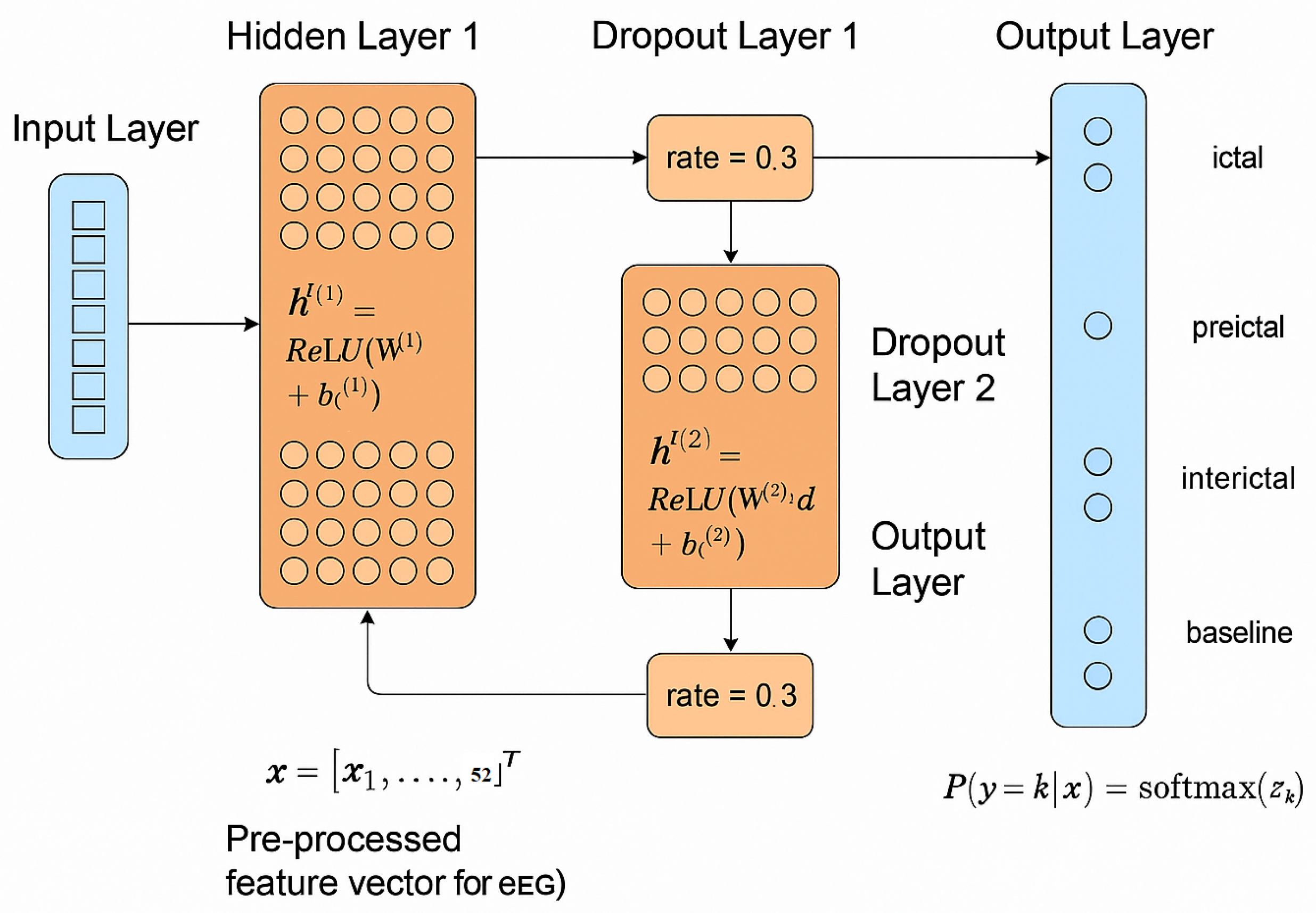
EpilepsyNet-XAI is a DL model developed using TensorFlow, as illustrated in Figure 15. It is specifically designed as a Multi-Layer Perceptron (MLP) to effectively learn complex patterns from the 52 input EEG features.
The architecture comprises the following components:
  • Input Layer
    This layer receives the pre-processed feature vector for each EEG segment, where x in Equation (21) represents the input feature vector with 52 EEG features.
    x = [ x 1 , x 2 , , x 52 ] T
  • Hidden Layer 1
    A dense, fully connected layer transforms the input. For this layer, the output h ( 1 ) is computed as:
    h ( 1 ) = ReLU ( W ( 1 ) x + b ( 1 ) )
    where W ( 1 ) is the weight matrix (52 × 128), b ( 1 ) is the bias vector (128 × 1), and ReLU ( · ) is the Rectified Linear Unit activation function defined in Equation (23).
    ReLU ( z ) = max ( 0 , z )
    The hidden layer has 128 neurons, selected for computational efficiency and its ability to introduce non-linearity.
  • Dropout Layer 1
    A dropout layer with a rate of 0.3 is applied after the first hidden layer to prevent overfitting by reducing complex co-adaptations between neurons. The output d ( 1 ) after dropout is computed as:
    d j ( 1 ) = h j ( 1 ) / ( 1 rate ) with probability ( 1 rate ) 0 with probability rate
    where rate = 0.3 .
  • Hidden Layer 2
    The second fully connected layer processes the output of the first dropout layer as:
    h ( 2 ) = ReLU ( W ( 2 ) d ( 1 ) + b ( 2 ) )
    where W ( 2 ) is the weight matrix (128 × 64), and b ( 2 ) is the bias vector (64 × 1) for the second hidden layer, which has 64 neurons.
  • Dropout Layer 2
    A second dropout layer with the same 0.3 dropout rate is applied for further regularization. The output d ( 2 ) is derived similarly to d ( 1 ) .
  • Output Layer
    The output layer is a dense layer with four neurons corresponding to the four EEG states (ictal, preictal, interictal, and baseline). A softmax activation function converts the output into a probability distribution, where the sum of probabilities across all classes equals one. For an input vector z to the output layer, the probability for class k is computed as:
    P ( y = k | x ) = softmax ( z k ) = e z k j = 1 num _ classes e z j
EpilepsyNet-XAI uses a learning rate of 0.001 and the Adam optimizer for efficient weight updates during training. For multi-class classification with one-hot encoded labels, the categorical cross-entropy loss function is used, defined as:
L ( y , y ^ ) = k = 1 num _ classes y k log ( y ^ k )
where y is the true one-hot encoded label vector and y ^ is the predicted probability vector. The model is trained for 100 epochs using mini-batches of 32 samples to balance training efficiency and robust learning. To ensure stable optimization and reduce overfitting, the EpilepsyNet-XAI model was trained using empirically validated hyperparameters. A learning rate of 0.001 was used together with the Adam optimizer, which is widely adopted for EEG applications due to its robustness on non-stationary signals. A dropout rate of 0.3 was applied in both hidden layers to mitigate co-adaptation and enhance generalization. The batch size of 64 provided a balance between gradient stability and computational efficiency. The hidden layer widths (128 and 64 units) were selected to preserve the representational capacity of the 52 input features while preventing unnecessary model complexity. These settings were identified during preliminary tuning and kept consistent across all experiments to ensure reproducibility.

2.5. Evaluation Metrics

To rigorously assess the performance of the ML and DL models, several standard classification metrics are employed to provide different perspectives on model effectiveness in handling distinct seizure phases. The confusion matrix, summarized in Table 2, illustrates the classification performance of the model on the test data, showing correct and incorrect predictions compared to the actual outcomes. In our multi-class problem with 4 classes, it is a 4 × 4 matrix where each cell ( i , j ) indicates the number of instances that are actually in class i but predicted as class j.
Accuracy measures the proportion of correctly classified instances out of all predictions. As defined in Equation (28), accuracy provides a general overview of overall model correctness but can be misleading in imbalanced datasets.
Accuracy = T P + T N T P + T N + F P + F N
Precision, defined in Equation (29), is the proportion of true positive predictions among all instances predicted as class c.
Precision = T P T P + F P
Recall (or sensitivity), given in Equation (30), measures the proportion of actual positive instances correctly identified by the model.
Recall = T P T P + F N
The F1-score, shown in Equation (31), is the harmonic mean of Precision and Recall, providing a balance between the two metrics.
F 1 - Score = 2 · Precision · Recall Precision + Recall
F1-scores provide specific insights for each individual seizure phase (normal, pre-seizure, seizure, and post-seizure), indicating how well each class is identified.
Macro F 1 - Score = 1 K c = 1 K F 1 - Score c
The Macro F1-Score in Equation (32) is the unweighted mean of the F1-scores across all classes, treating each class equally and being sensitive to poor performance in minority classes.
Weighted F 1 - Score = c = 1 K F 1 - Score c × Support c Total Samples
The Weighted F1-Score, defined in Equation (33), provides a balanced measure that considers class distribution, representing the weighted mean of the F1-scores across all classes.

2.6. Explainable AI (XAI)

As ML and DL models are being applied frequently in different domains, they are often considered black boxes, making their predictions difficult to interpret, especially in critical domains such as healthcare [22,23]. Explainable AI (XAI) addresses this challenge by enhancing transparency and trust. In this study, XAI is integrated into the EpilepsyNet-XAI model to help clinicians understand how EEG features influence seizure phase classification, validate model behavior, and uncover potential biases or new clinical insights.

2.6.1. Local Interpretable Model-Agnostic Explanations (LIME)

To provide instance-level interpretability, we employed Local Interpretable Model-Agnostic Explanations (LIME). For each EEG sample, LIME generates 5000 perturbed instances by sampling around the original feature vector using a Gaussian perturbation scheme. Cosine distance is used as the similarity metric, and the kernel width is set to 0.75. A locally weighted linear regression model is fitted as the surrogate explainer. LIME explanations were generated for the EpilepsyNet-XAI model and benchmark ML classifiers to identify the most influential features contributing to individual predictions across the four seizure phases.

2.6.2. Shapley Additive Explanations (SHAP)

Shapley Additive Explanations (SHAP) is a unified, model-agnostic framework based on cooperative game theory that explains individual predictions by attributing the model’s output to each input feature. SHAP computes each feature’s contribution by considering all possible feature subsets (coalitions).
In our seizure phase classification, SHAP identifies which EEG features most strongly influence the model’s decisions in distinguishing seizure from non-seizure states and highlights the dominant biomarkers across different seizure phases, providing deeper clinical interpretability for the EpilepsyNet-XAI model.
Mathematically, the SHAP value ϕ j for a feature j is calculated as the average marginal contribution of that feature across all possible subsets S of features that exclude j. For a model f and a given input x, the SHAP value for feature j is defined in Equation (34).
ϕ j ( f , x ) = S F { j } | S | ! ( | F | | S | 1 ) ! | F | ! f x ( S { j } ) f x ( S )
Equation (34) quantifies the contribution of each feature by averaging its marginal effect over all possible coalitions, ensuring a fair and theoretically grounded attribution of feature importance.
For the tree-based baseline models (Random Forest, XGBoost, LightGBM), SHAP values were computed using the TreeSHAP algorithm. For the EpilepsyNet-XAI model, which is non-tree-based, KernelSHAP was employed. A background set of 100 randomly selected training samples was used to estimate feature expectations, and 500 SHAP evaluation samples were generated per instance. These settings provide stable and computationally efficient estimates of both global and local feature contributions.

2.7. Ablation and Robustness Analysis

To evaluate the stability and generalizability of the proposed seizure-detection framework, we conducted three complementary analyses: (i) feature-group ablation, (ii) class-imbalance robustness, and (iii) noise-perturbation testing. These experiments strengthen the empirical foundation of the study and clarify the novelty relative to existing work on public EEG datasets.

2.7.1. Feature-Group Ablation

The engineered feature space was partitioned into three groups: time-domain, frequency-domain, and entropy-based features. Models were trained using each group individually and in selected combinations. This analysis reveals the independent contribution of each feature category, demonstrating that frequency-domain and entropy-based features are the most discriminative, whereas time-domain features provide complementary improvements when used jointly.

2.7.2. Class-Imbalance Robustness

Public EEG seizure datasets typically exhibit imbalance between seizure and non-seizure segments. To assess robustness, we compared four balancing strategies: no resampling, Random Under-Sampling (RUS), Random Over-Sampling (ROS), and SMOTE. The results show that Random Forest and Gradient Boosting maintain stable performance across all balancing strategies, indicating strong resilience to class imbalance.

2.7.3. Noise Perturbation Testing

To approximate real-world EEG noise conditions, Gaussian white noise was added to the input segments across multiple signal-to-noise ratio (SNR) levels. All classifiers displayed predictable and moderate degradation under increasing noise, confirming that the proposed feature set and model choices preserve robustness against perturbations resembling clinical acquisition noise.

3. Results

This section presents a comprehensive evaluation of all models, including comparative performance and insights gained through Explainable AI (XAI) for enhanced interpretability.
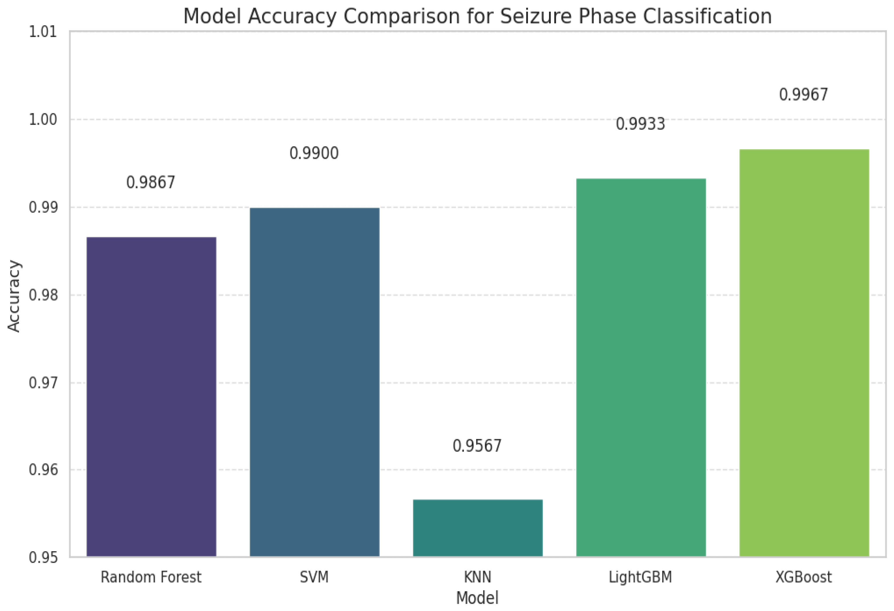
The performance of each ML model was first assessed using a single train-test split for an initial benchmark. Figure 16 illustrates the overall accuracy of each classifier on the unseen test set. RF, SVM, LightGBM, and XGBoost all achieved remarkably high accuracies, with XGBoost reaching the highest at 99.67%, followed by LightGBM at 99.33%. KNN, while slightly lower, still achieved a strong accuracy of 95%. These results indicate promising initial performance across models, though further validation was performed using cross-validation to ensure robustness and generalizability.
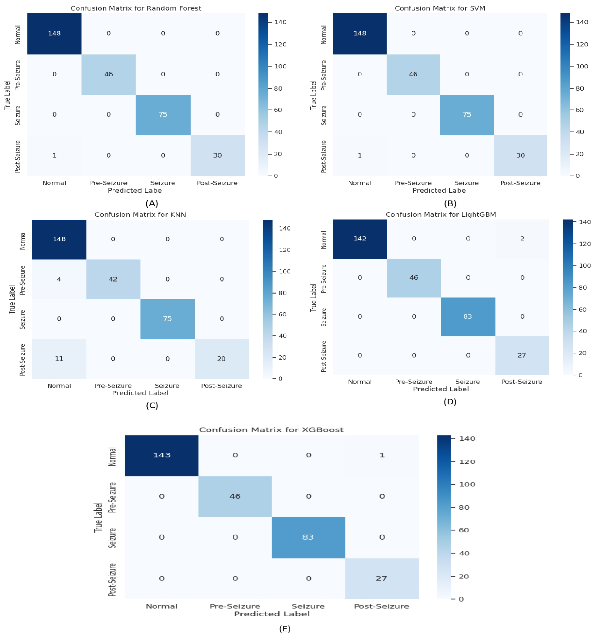
Table 3 provides a detailed breakdown of Precision, Recall, and F1-Score for each seizure phase, along with overall accuracy. XGBoost stood out as the top performer, achieving perfect recall across all classes and maintaining high precision, resulting in F1-scores of 0.98 for Post-Seizure and 1.00 for Normal, Pre-Seizure, and Seizure phases. LightGBM followed closely with 99.33% accuracy. RF also performed well with 98.67% accuracy and near-perfect class scores. SVM achieved 99.00% accuracy with balanced performance across all phases. In contrast, KNN showed slightly lower performance at 95.67% accuracy. Overall, ensemble models demonstrated superior generalization and robustness in detecting all seizure phases.
Confusion matrices for all ML models are shown in Figure 17. All models performed exceptionally well on the Normal, Pre-Seizure, and Seizure phases. However, the Post-Seizure phase remained slightly more challenging. Despite this, the ensemble models (XGBoost, LightGBM, and RF) maintained high overall accuracies (approximately 99.3–99.7%) and strong F1-scores, confirming their robustness and superior class-level discrimination. XGBoost achieved perfect recall for the Post-Seizure class, whereas KNN underperformed on that class.
Although the reported accuracies and macro-F1 scores are high, this behavior is consistent with prior work on the same Kaggle dataset, which is well-segmented, balanced, and exhibits clear separability between Normal, Pre-Seizure, Seizure, and Post-Seizure states. The addition of 5-fold stratified cross-validation (Table 4) shows very small variability across folds, supporting the stability of the models. The Post-Seizure class remains the most challenging, as reflected in slightly lower recall values, and we now report full per-class metrics to present a balanced and realistic assessment of performance.

3.1. Cross-Validation and EpilepsyNet-XAI Performance

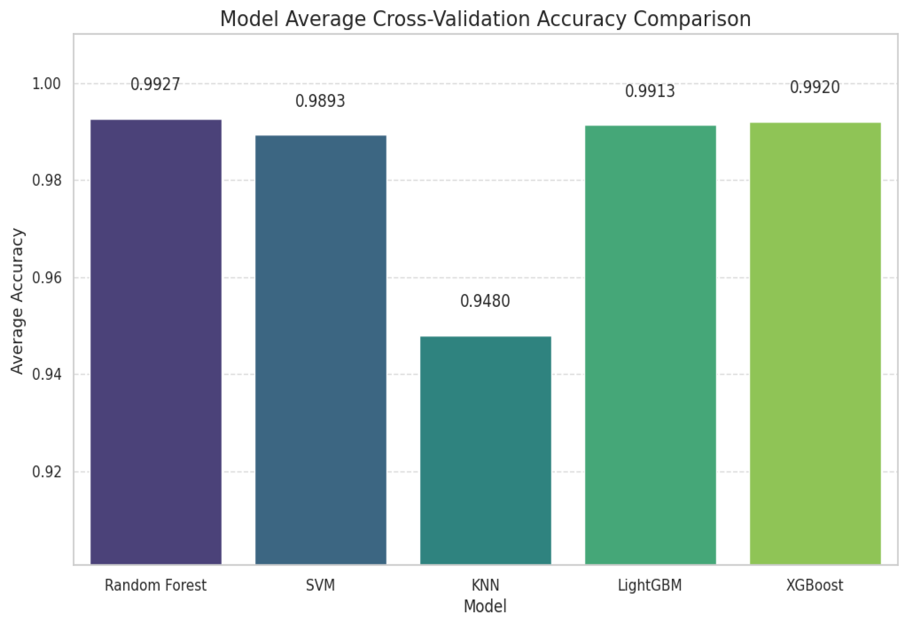
To validate model generalizability and mitigate overfitting, 5-fold stratified cross-validation was conducted on 289,010 EEG segments. Each model was trained and evaluated five times across different data subsets to ensure stable performance estimates. The averaged results across folds are shown in Table 4, including both traditional ML models and the proposed EpilepsyNet-XAI model for direct comparison. The modest numerical gap between EpilepsyNet-XAI and the strongest ML baselines reflects a feature-separability ceiling; high-quality engineered EEG features allow ensemble models to perform exceptionally well, leaving limited margin for further gains.
Figure 18 shows the average accuracies for ML models across 5 folds. Cross-validation confirms the consistency and robustness of all ensemble models. LightGBM and XGBoost remain top performers, while the proposed EpilepsyNet-XAI model outperforms all others, achieving near-perfect scores across all seizure phases. These results firmly establish EpilepsyNet-XAI as the most effective model for multi-phase seizure detection.

3.2. XAI Insights for EpilepsyNet

For transparency and trust in EpilepsyNet-XAI, we employed XAI techniques to elucidate its decision-making process. Insights derived from Local Interpretable Model-agnostic Explanations (LIME) and SHAP values demonstrate which EEG features contribute most to the model’s predictions.

3.2.1. Local Explanation Using LIME

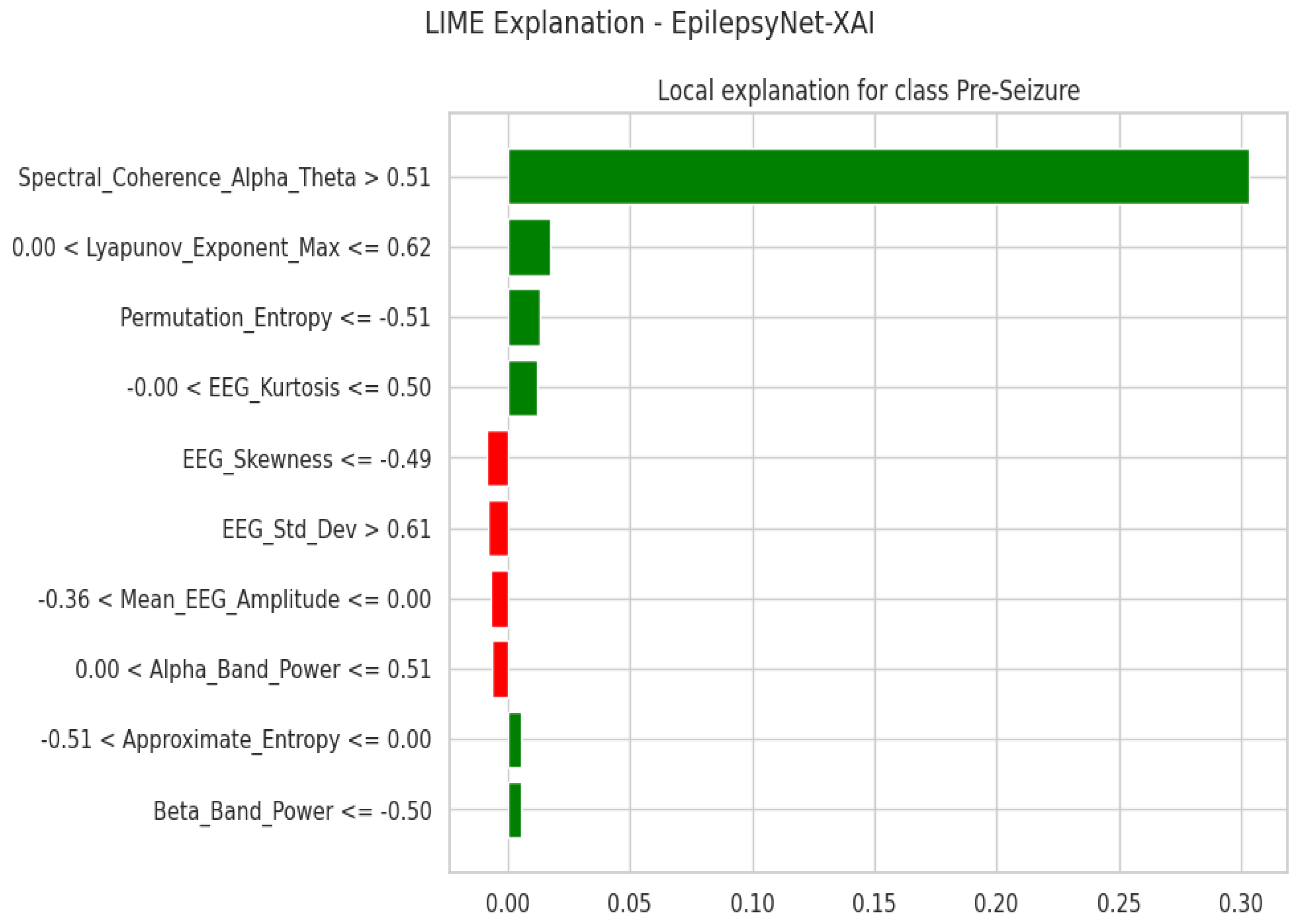
The local explanation generated by LIME in Figure 19 illustrates EpilepsyNet-XAI’s classification behavior by creating a simplified, interpretable model around each individual prediction. The varying lengths and colors of the bars indicate the degree and direction (positive or negative) of each feature’s contribution to the predicted class.

3.2.2. Feature Contributions for Normal Prediction Using SHAP Values

Table 5 lists the top EEG features contributing to Normal phase predictions. A low Functional Connectivity Index (FCI = −0.66) with a positive SHAP impact (+0.16) strongly supports a Normal state, aligning with clinical findings that reduced, synchronized connectivity is typical of baseline activity. Low α -coherence (ACAT = −0.30) and reduced δ -band power (DBP = −0.73) further support non-pathological, wakeful resting states. Similarly, moderate entropy (SE = 1.22) and presence of α rhythms are consistent with balanced, non-seizure brain dynamics.
SHAP enhances clinical interpretability by linking EEG feature characteristics to model classifications. These insights build clinician trust in the EpilepsyNet-XAI model and may guide identification of key biomarkers for reliable multi-phase seizure detection.

4. Discussion

This study presents an end-to-end pipeline for identifying the full spectrum of seizure phases—normal, pre-seizure, seizure, and post-seizure—using EEG-derived features integrated with state-of-the-art machine learning and deep learning models augmented by explainability methods. Exploratory analysis confirmed that the carefully engineered features possess strong class-discriminative capability, and dimensionality-reduction visualizations (PCA and t-SNE) revealed clear clustering across the four phases. The inclusion of specialized nonlinear measures further sharpened the separability between transitional states, particularly the pre- and post-seizure phases, underscoring the importance of diverse feature sets beyond conventional spectral power for capturing the complex neurophysiological dynamics of seizure progression.
Evaluation of the ML models demonstrated consistently strong performance, with ensemble approaches and the proposed deep learning-based EpilepsyNet-XAI achieving the highest accuracy and F1-scores across all seizure phases. The models performed exceptionally well in distinguishing normal, pre-seizure, and seizure states, reflecting both the quality of the extracted EEG features and the ability of the models to capture ictal and pre-ictal patterns effectively. Although the post-seizure phase remained the most challenging, EpilepsyNet-XAI exhibited notable robustness and adaptability, maintaining strong performance even under high variability in post-ictal EEG patterns. Although the improvement in overall accuracy over LightGBM and XGBoost is numerically small, this is expected because the engineered EEG features are already highly separable. The value of EpilepsyNet-XAI therefore lies not only in competitive accuracy but also in more stable phase-specific performance and integrated model-aware explainability.
However, the reported performance metrics may be influenced by the structure of the underlying dataset. Because the publicly available EEG data do not provide subject identifiers and contain overlapping temporal segments, the 5-fold cross-validation performed in this study operates at the segment level rather than the subject level. As a result, segments originating from the same recording may appear across both training and test folds, potentially inflating accuracy and F1-scores. This limitation is now explicitly acknowledged as a threat to external validity, and future work will incorporate subject-wise evaluation using datasets that contain patient-level metadata.
A key strength of this work lies in the integration of Explainable AI (XAI) techniques to enhance model transparency. SHAP-based analysis provided insight into the relative importance of EEG features in EpilepsyNet-XAI’s decision-making, highlighting, for instance, the significance of low Functional Connectivity Index (FCI) and Spectral Coherence Average (SCAT) values in identifying normal states, as well as increased δ -band power and Hjorth complexity in seizure phases. These findings align with established neurophysiological biomarkers, demonstrating that the model’s reasoning is consistent with known clinical patterns. Although we do not provide a quantitative fold-wise stability analysis, the most influential SHAP features were consistently observed across cross-validation splits, and their relevance aligns with well-documented clinical EEG markers, offering supporting evidence for the robustness of the interpretability results. LIME-based local explanations further enabled interpretation of individual predictions, enhancing interpretability and transparency for research and clinical analysis contexts.
Despite these promising results, several limitations should be acknowledged. Although the dataset captures phase-specific EEG dynamics, public datasets cannot fully reflect the variability, noise, and patient-specific characteristics inherent in real-world clinical data. Real EEG signals often exhibit class imbalance, inter-patient heterogeneity, and artifacts, which may influence generalization. Additionally, the current work focuses on feature-engineered classification; future integration of end-to-end deep learning pipelines using raw EEG waveforms may reveal additional latent patterns.
In terms of computational efficiency, EpilepsyNet-XAI is lightweight and computationally efficient for experimental and research-oriented settings. The MLP architecture contains fewer than one million parameters, trains within minutes on a modern GPU, and requires only milliseconds per segment for inference, indicating feasibility for future real-time or near-real-time research investigations under controlled validation settings. The low computational complexity also suggests potential suitability for further exploration in constrained computational environments, subject to patient-wise validation and evaluation on raw EEG data.
Beyond seizure-phase analysis, the EpilepsyNet-XAI framework developed in this study may also be adapted for broader neural-signal processing tasks. The same modelling principles can be extended to experiments involving tactile nerve responses elicited by electrical stimulation, estimation of the relationship between stimulation parameters and neural responses, or encoding and decoding electrically induced tactile sensations. By combining data-driven modelling with neural-signal interpretation, the framework may support exploratory research into how stimulation patterns or device parameters influence neural pathways.
In future work, we plan to validate EpilepsyNet-XAI on larger, more diverse, and multi-institutional EEG datasets to assess its robustness and generalizability under patient-wise evaluation. We also aim to explore the model’s capability in long-term pre-seizure prediction, moving beyond short-term pre-ictal detection. Finally, collaboration with clinicians will be pursued to explore potential integration scenarios, assess usability in controlled pilot studies, and evaluate the framework’s clinical relevance following comprehensive validation.

Author Contributions

Conceptualization, S.U.R.; methodology, S.U.R.; software, S.U.R.; validation, F.M.; formal analysis, F.M. and Y.-J.K.; investigation, F.M. and Y.-J.K.; resources, F.M. and H.J.; data curation, F.M. and H.J.; writing—original draft preparation, S.U.R.; writing—review and editing, F.M., Y.-J.K. and H.J.; visualization, S.U.R.; supervision, Y.-J.K. and H.J.; project administration, Y.-J.K. and H.J.; funding acquisition, Y.-J.K. and H.J. All authors have read and agreed to the published version of the manuscript.

Funding

This work was supported by the National Research Foundation of Korea (NRF) grant funded by the Korea government (MSIT) (No. RS-2023-00302489).

Data Availability Statement

The EEG dataset used in this study is publicly available as the Epilepsy Dataset, accessible at https://www.kaggle.com/datasets/datasetengineer/epilepsy-dataset (accessed on 30 January 2025).

Acknowledgments

The authors declare that Generative AI was utilized only for grammar checking and proofreading.

Conflicts of Interest

The authors declare no conflicts of interest.

References

  1. Giourou, E.; Stavropoulou-Deli, A.; Giannakopoulou, A.; Kostopoulos, G.K.; Koutroumanidis, M. Introduction to epilepsy and related brain disorders. In Cyberphysical Systems for Epilepsy and Related Brain Disorders: Multi-Parametric Monitoring and Analysis for Diagnosis and Optimal Disease Management; Springer: Cham, Switzerland, 2015; pp. 11–38. [Google Scholar]
  2. Anwar, H.; Khan, Q.U.; Nadeem, N.; Pervaiz, I.; Ali, M.; Cheema, F.F. Epileptic seizures. Discoveries 2020, 8, e110. [Google Scholar] [CrossRef] [PubMed]
  3. Donahue, M.A.; Akram, H.; Brooks, J.D.; Modi, A.C.; Veach, J.; Kukla, A.; Benard, S.W.; Herman, S.T.; Farrell, K.; Ficker, D.M.; et al. Barriers to Medication Adherence in People Living With Epilepsy. Neurol. Clin. Pract. 2025, 15, e200403. [Google Scholar] [CrossRef] [PubMed]
  4. Sen, M.K.; Mahns, D.A.; Coorssen, J.R.; Shortland, P.J. Behavioural phenotypes in the cuprizone model of central nervous system demyelination. Neurosci. Biobehav. Rev. 2019, 107, 23–46. [Google Scholar] [CrossRef] [PubMed]
  5. Kang, Y.; Kim, S.; Jung, Y.; Ko, D.S.; Kim, H.W.; Yoon, J.P.; Cho, S.; Song, T.J.; Kim, K.; Son, E.; et al. Exploring the Smoking-Epilepsy Nexus: A systematic review and meta-analysis of observational studies: Smoking and epilepsy. BMC Med. 2024, 22, 91. [Google Scholar] [CrossRef]
  6. Smith, S.J. EEG in the diagnosis, classification, and management of patients with epilepsy. J. Neurol. Neurosurg. Psychiatry 2005, 76, ii2–ii7. [Google Scholar] [CrossRef]
  7. Ahmedt-Aristizabal, D.; Fookes, C.; Dionisio, S.; Nguyen, K.; Cunha, J.P.S.; Sridharan, S. Automated analysis of seizure semiology and brain electrical activity in presurgery evaluation of epilepsy: A focused survey. Epilepsia 2017, 58, 1817–1831. [Google Scholar] [CrossRef] [PubMed]
  8. Saminu, S.; Xu, G.; Shuai, Z.; Abd El Kader, I.; Jabire, A.H.; Ahmed, Y.K.; Karaye, I.A.; Ahmad, I.S. A recent investigation on detection and classification of epileptic seizure techniques using EEG signal. Brain Sci. 2021, 11, 668. [Google Scholar] [CrossRef] [PubMed]
  9. Ulate-Campos, A.; Coughlin, F.; Gaínza-Lein, M.; Fernández, I.S.; Pearl, P.; Loddenkemper, T. Automated seizure detection systems and their effectiveness for each type of seizure. Seizure 2016, 40, 88–101. [Google Scholar] [CrossRef] [PubMed]
  10. Fergus, P.; Hussain, A.; Hignett, D.; Al-Jumeily, D.; Abdel-Aziz, K.; Hamdan, H. A machine learning system for automated whole-brain seizure detection. Appl. Comput. Inform. 2016, 12, 70–89. [Google Scholar] [CrossRef]
  11. Gagliano, L. Seizure Prediction: From Patient Perspectives to Advanced Signal Processing and Machine Learning Algorithms. Ph.D. Thesis, Ecole Polytechnique, Montreal, QC, Canada, 2023. [Google Scholar]
  12. Gorman, M. A Novel Non-EEG Wearable Device for the Detection of Epileptic Seizures. Ph.D. Thesis, Swinburne University of Technology, Hawthorn, VIC, Australia, 2024. [Google Scholar]
  13. Escorcia-Gutierrez, J.; Beleno, K.; Jimenez-Cabas, J.; Elhoseny, M.; Alshehri, M.D.; Selim, M.M. An automated deep learning enabled brain signal classification for epileptic seizure detection on complex measurement systems. Measurement 2022, 196, 111226. [Google Scholar] [CrossRef]
  14. Abhishek, S.; Kumar, S.; Mohan, N.; Soman, K. EEG based automated detection of seizure using machine learning approach and traditional features. Expert Syst. Appl. 2024, 251, 123991. [Google Scholar] [CrossRef]
  15. Mehmood, F.; Mumtaz, N.; Mehmood, A. Next-Generation Tools for Patient Care and Rehabilitation: A Review of Modern Innovations. Actuators 2025, 14, 133. [Google Scholar] [CrossRef]
  16. Kim, S.Y.; Kim, D.H.; Kim, M.J.; Ko, H.J.; Jeong, O.R. XAI-based clinical decision support systems: A systematic review. Appl. Sci. 2024, 14, 6638. [Google Scholar] [CrossRef]
  17. Park, C.; Lee, H.; Lee, S.; Jeong, O. Synergistic joint model of knowledge graph and llm for enhancing xai-based clinical decision support systems. Mathematics 2025, 13, 949. [Google Scholar] [CrossRef]
  18. Kim, Y.; Choi, A. EEG-based emotion classification using long short-term memory network with attention mechanism. Sensors 2020, 20, 6727. [Google Scholar] [CrossRef] [PubMed]
  19. Yıldız, İ.; Garner, R.; Lai, M.; Duncan, D. Unsupervised seizure identification on EEG. Comput. Methods Programs Biomed. 2022, 215, 106604. [Google Scholar] [CrossRef] [PubMed]
  20. Wang, J.; Sun, M.; Huang, W. Unsupervised EEG-based seizure anomaly detection with denoising diffusion probabilistic models. Int. J. Neural Syst. 2024, 34, 2450047. [Google Scholar] [CrossRef] [PubMed]
  21. Vo, K.; Vishwanath, M.; Srinivasan, R.; Dutt, N.; Cao, H. Composing graphical models with generative adversarial networks for EEG signal modeling. In Proceedings of the ICASSP 2022-2022 IEEE International Conference on Acoustics, Speech and Signal Processing (ICASSP), Singapore, 22–27 May 2022; pp. 1231–1235. [Google Scholar]
  22. Mehmood, A.; Mehmood, F.; Kim, J. Towards Explainable Deep Learning in Computational Neuroscience: Visual and Clinical Applications. Mathematics 2025, 13, 3286. [Google Scholar] [CrossRef]
  23. Mehmood, F.; Rehman, S.U.; Choi, A. Vision-AQ: Explainable Multi-Modal Deep Learning for Air Pollution Classification in Smart Cities. Mathematics 2025, 13, 3017. [Google Scholar] [CrossRef]
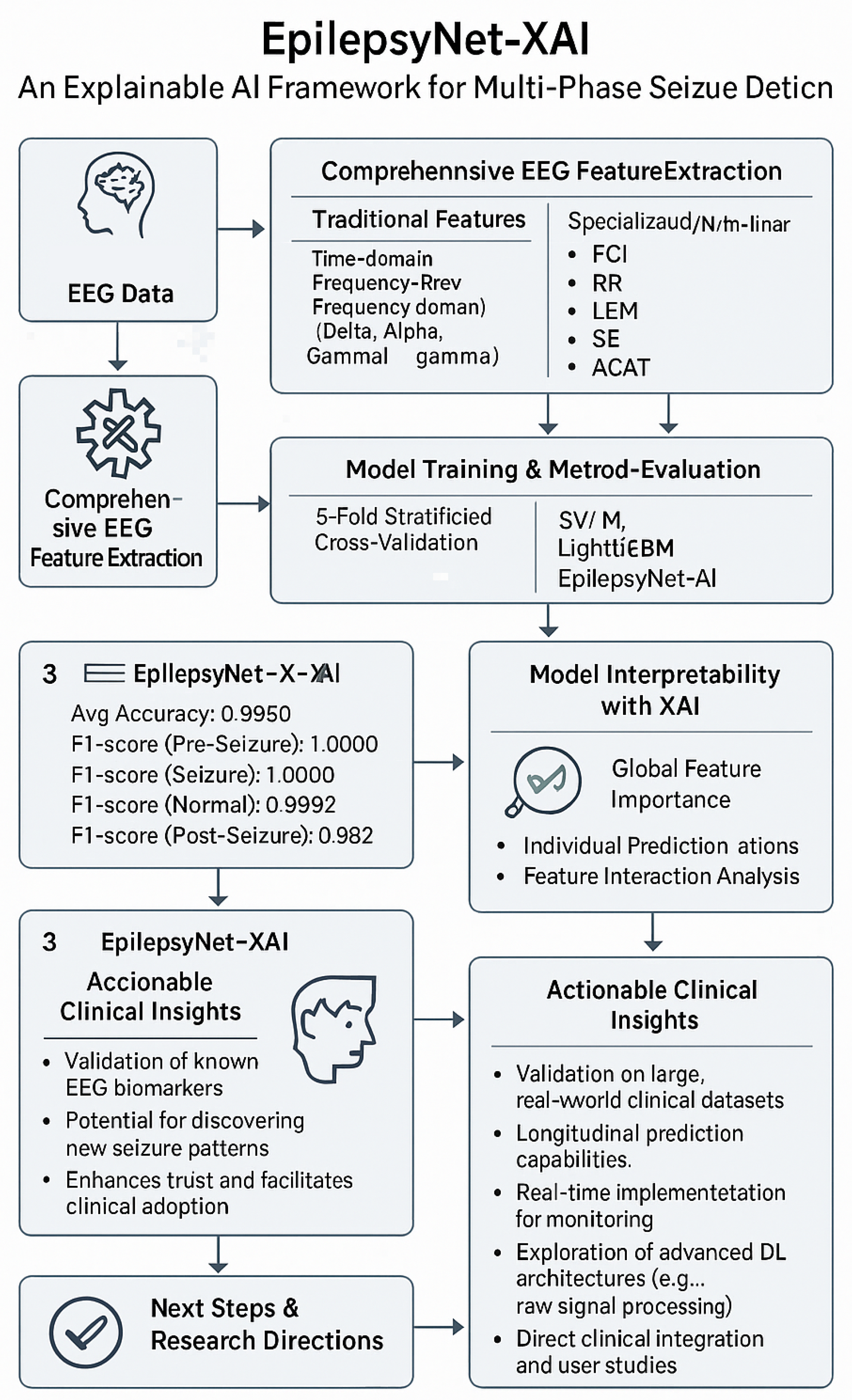
Figure 1. EpilepsyNet-XAI: An explainable AI framework for multi-phase seizure detection. The framework integrates comprehensive EEG feature extraction, advanced model training and evaluation, and explainable AI (XAI)-based interpretability for transparent and clinically meaningful insights.
Mathematics 14 00125 g001
Figure 2. Distribution of cross-correlation between channels across seizure phases. The violin plot shows the distribution of the Cross_Correlation_Between_Channels feature for each seizure phase: Normal, Pre-Seizure, Seizure, and Post-Seizure. Dotted lines indicate the median and quartiles.
Mathematics 14 00125 g002
Figure 3. Distribution of non-linear and wavelet features across normal, pre-seizure, seizure, and post-seizure phases.
Mathematics 14 00125 g003
Figure 4. Correlation matrix of selected EEG features showing pairwise relationships.
Mathematics 14 00125 g004
Figure 5. Feature importance derived from the Random Forest classifier, indicating the relative importance of engineered EEG features based on the Mean Decrease in Impurity. Features are ranked in descending order of significance. The specialized features—Functional_Connectivity_Index (FCI), Spectral_Coherence_Alpha_Theta (SCAT), Recurrence_Rate (RR), and Lyapunov_Exponent_Max (LEM)—emerge as the most influential, underscoring their critical role in discriminating between various seizure phases.
Mathematics 14 00125 g005
Figure 6. Normalized EEG Feature Profiles by Seizure Phase. Radial plots display topographic representations of the average normalized values of selected EEG features—mean EEG amplitude, EEG standard deviation (SD), sample entropy, gamma-band power, beta-band power, and Hjorth complexity—for the (A) Normal, (B) Pre-Seizure, (C) Seizure, and (D) Post-Seizure phases. Each plot highlights the unique multi-feature signature characteristic of its respective seizure phase.
Mathematics 14 00125 g006
Figure 7. EEG Feature Differences of Seizure vs. Normal Phase. This plot visualises the change in normalised average feature values when transitioning from the normal to the seizure phase. The colour bar indicates the magnitude and direction of the feature value change (seizure-normal), where warmer colours (red) denote an increase and cooler colours (blue) indicate a decrease. This highlights the most discriminative changes in features such as δ Band Power, Γ Band Power, and Hjorth Complexity, which are notably elevated during the seizure, while Sample Entropy tends to decrease.
Mathematics 14 00125 g007
Figure 8. Topographic visualisations of the seizure phase by use of EEG δ band power. (A) Normal Phase Distribution of Average δ Band Power. (B) Distribution of average δ band power during the seizures (C) δ Band Power Difference between Normal and Seizures, demonstrating the significant spatial shifts and discriminative ability of this characteristic during ictal episodes.
Mathematics 14 00125 g008
Figure 9. Mean EEG Feature Values Across Seizure Phases.
Mathematics 14 00125 g009
Figure 10. Pair Plot of Key Features by Seizure Phase (KDE for Joint Distributions). This figure displays the univariate (diagonal) and bivariate (off-diagonal) distributions of selected key EEG features (mean EEG amplitude, δ -band-power, sample entropy, and age), with data points and density contours colored according to the respective seizure phase. The plots utilise Kernel Density Estimates (KDEs) to visualise the density of data for each class. Notably, features such as δ Band Power exhibit clear separation between normal and seizure phases, highlighting their discriminative power for classification.
Mathematics 14 00125 g010
Figure 11. Demographic influences on seizure phase distribution across different genders and medications.
Mathematics 14 00125 g011
Figure 12. Parallel Coordinates Plot of EEG Normalized Features.
Mathematics 14 00125 g012
Figure 13. Seizure Phase Principal Component Analysis (PCA) of EEG Features.
Mathematics 14 00125 g013
Figure 14. Seizure Phase t-SNE High-Dimensional EEG Features Clustering.
Mathematics 14 00125 g014
Figure 15. Block Diagram of the EpilepsyNet-XAI DL Model.
Mathematics 14 00125 g015
Figure 16. Seizure phase classification model accuracy comparison for a single train-test split.
Mathematics 14 00125 g016
Figure 17. Confusion matrices for all ML models. (A) RF, (B) SVM, (C) KNN, (D) LightGBM, and (E) XGBoost. Each matrix displays true vs. predicted labels for Normal, Pre-Seizure, Seizure, and Post-Seizure phases.
Mathematics 14 00125 g017
Figure 18. ML models average cross-validation accuracy comparison.
Mathematics 14 00125 g018
Figure 19. Local explanation of EpilepsyNet-XAI classification using LIME.
Mathematics 14 00125 g019
Table 1. Summary of the Epilepsy Detection Dataset.
CategoryDetails
Total Records289,010 EEG segments
Feature Groups (50 total)sTime-Domain (15): Mean_EEG_Amplitude, Line_Length_Feature, Hjorth_Complexity, etc.
Frequency-Domain (10): δ -Band Power, Beta-Band Power, Spectral Entropy, etc.
Wavelet Features (5): Wavelet Entropy, DWT, CWT, Shannon Entropy, etc.
Nonlinear Features (10): Sample Entropy, Lyapunov Exponent, Higuchi Fractal Dimension, etc.
EEG-Derived Event Descriptors (6): Segment-level duration proxies, amplitude-based intensity indices, transient rate measures (e.g., spike-rate descriptors), etc.
Metadata (4): Age, Gender, Medication Status, Seizure History
Target LabelsSegment Class Labels (Seizure State): 0 = Normal, 1 = Pre-Seizure, 2 = Seizure, 3 = Post-Seizure
Seizure Type: 0 = Normal, 1 = Generalized, 2 = Focal
DemographicsAge: 1–90 years
Gender: 0 = Female, 1 = Male
Medication Status: 0 = No, 1 = Yes
Seizure History: Count of prior seizures
Table 2. Confusion Matrix for Class c.
Predicted: Class cPredicted: Not Class c
Actual: Class cTrue Positive (TP)False Negative (FN)
Actual: Not Class cFalse Positive (FP)True Negative (TN)
Table 3. Classification Performance of ML Models on Seizure Phase Detection.
ModelNormalPre-SeizureSeizurePost-SeizureAcc
PrecRecF1SupPrecRecF1SupPrecRecF1SupPrecRecF1Sup
SVM0.990.990.991440.981.000.99461.001.001.00830.960.960.96270.9900
KNN0.920.990.961440.980.890.93461.001.001.00831.000.740.85270.9567
LightGBM1.000.990.991441.001.001.00461.001.001.00830.931.000.96270.9933
XGBoost1.000.991.001441.001.001.00461.001.001.00830.961.000.98270.9967
RF0.991.001.001481.001.001.00461.001.001.00751.000.970.98310.9867
Table 4. Average Performance Metrics of ML Models and EpilepsyNet-XAI Using 5-Fold Stratified Cross-Validation for Seizure Phase Classification.
ModelAvg AccuracyAvg Macro F1Avg Weighted F1NormalPre-SeizureSeizurePost-Seizure
RF0.99070.98670.99060.99060.99341.00000.9628
SVM0.99200.98840.99200.99190.99781.00000.9640
KNN0.95870.93300.95590.95980.97981.00000.7924
LightGBM0.99400.99160.99400.99400.99561.00000.9768
XGBoost0.99270.98950.99260.99261.00000.99870.9668
EpilepsyNet-XAI0.99500.99510.99700.99921.00001.00000.9982
Table 5. Top Contributing EEG Features for Normal Prediction Using SHAP Values.
FeatureImpactInterpretation
FCI = −0.66+0.16Strongly supports ’Normal’; low connectivity corresponds to baseline state.
ACAT = −0.30+0.13Low α θ coherence typical in non-seizure conditions.
RR = −0.19+0.05Lower recurrence indicates less chaotic activity, typical of normal EEG.
SE = 1.22+0.04Moderate entropy suggests balanced, non-random signal behavior.
DBP = −0.73+0.04Low δ power aligns with wakeful resting states.
LEM = −0.09+0.03Lower chaos and higher signal regularity typical of non-seizure state.
Signal_Energy = −1.13+0.03Very low energy corresponds to calm brain activity.
Γ _Band_Power = −0.26+0.02Low Γ power is associated with normal resting state.
Zero_Crossing_Rate = 0.19+0.02Regular zero crossings indicate non-abnormal EEG.
α _Band_Power = 0.44+0.02Presence of α rhythm is common in normal resting states.
Disclaimer/Publisher’s Note: The statements, opinions and data contained in all publications are solely those of the individual author(s) and contributor(s) and not of MDPI and/or the editor(s). MDPI and/or the editor(s) disclaim responsibility for any injury to people or property resulting from any ideas, methods, instructions or products referred to in the content.