On Some Novel Uses of Strain Tensors Beyond Visualization in Modern Shape Analysis

Abstract

Modern Shape Analysis integrates mathematical and statistical methods to study morphology using geometric data from 2D and 3D digitization. Beyond visualization, local deformation analysis offers deeper insight into longitudinal changes like ontogenetic growth. This study explores strain tensors as analytical tools for shape transformations, evaluating Thin Plate Spline, Quadratic Trend, and Cubic Trend interpolants in estimating deformation tensors at landmarks. Simulated 2D data and 3D hominid skulls confirm that tensor-based multivariate analyses, such as Principal Component Analysis, yield results comparable to Parallel Transport methods. Thin Plate Spline more accurately recovers assigned tensors than least square interpolants, making it preferable for local deformation analysis. This method integrates traditional shape comparisons, proving particularly useful for studying ontogenetic trajectories and biomechanical deformations.

1. Introduction

This paper focuses on showcasing the effectiveness of a new approach for studying multigroup longitudinal deformations by inputting deformation strain tensor components in linear ordination analyses, achieving performances comparable to selecting a Riemannian connection and metric in a Parallel Transport procedure. Our work equally targets developers of mathematical and statistical protocols from a methodological perspective and the life sciences research community, in its broadest sense, from paleobiology to clinical research. Current Modern Shape Analysis (MSA) exploits the potential of a vast array of numerical, mathematical, and statistical methods [1]. All these approaches use coordinates (often Cartesian) to represent simulated (analytically/computationally generated) or real forms (shapes and their sizes). In the life sciences, spanning from paleontology to clinical research, raw data are used to digitize/re-digitize manually, semi-automatically, or fully automatically the positions of (ideally) anatomically homologous landmarks on acquired body shapes, aiming to capture comparable locations on anatomical structures with the same evolutionary or embryogenetic origin. Given the elusive nature of anatomical homology when applied to a dimensionless geometric entity such as a single point, researchers typically accept the compromise of assigning to it the status of a homologous landmark. The degree of histological, embryological, and evolutionary homology of a given landmark is often categorized using different “types” of digitized landmarks (e.g., Type I to VI; [2]) based on their (un)ambiguous embryogenetic origin and recognizability in biological tissues.

In cases where curves or surfaces need to be digitized, the semilandmarks technique is commonly employed, allowing points to slide between fixed landmarks [3], optionally minimizing Procrustes distance or bending energy. A landmark-free approach, such as Fourier analysis, provides an alternative for contour-based analyses [4].

Under the point’s correspondence/homology paradigm, the final data consists of a collection of n matrices, each of dimension $k\times m$ with n the number of individuals, k the number of landmarks, and m the number of dimensions (with $m\in \{2,3\}$ in the real physical world). Alternatively, some methods can completely abandon point correspondence for shape comparison and instead leverage specialized diffeomorphic approaches, such as Large Diffeomorphic Deformation Metric Mapping (LDDMM; [5] and references therein).

The fate of these coordinates varies significantly depending on the statistical and computational approaches used today, ranging from simple inter-landmark distance calculations (EDMA) to MSA under different paradigms, including Geometric Morphometrics (GM), Diffeomorphisms, and Continuum Mechanics (CM).

Scaling or non-scaling forms at unit size and alignment criteria for finding a mean shape are matters of arbitrary choices that in recent years have been challenged in several contributions [6,7], especially for defining size as centrod size (CS) or m-Volume. While scaling shapes aligned with their mean leads to a shape space (SS), not doing so leads to a size and shape space (SSS).

The resulting coordinates can then be subjected to various ordination analyses such as Principal Component Analysis (PCA), Linear Discriminant Analysis (LDA), Partial Least Squares (PLS), and regression/factor analyses against independent variables (e.g., size, age/time, environmental parameters, clinical indicators, categorical variables), and various measures of integration [6], among others.

Very often, the longitudinal morphological evolution of different bodies changing shape and size in time is the object of investigations that deal with group-wise morphological trajectories, each constituted by a series of forms/shapes acquired at different times. Besides ontogenetic data in a variety of organisms, the cardiac revolution is a paradigmatic example [8]. It could be of interest to explore differences in deformative processes rather than in form/shapes per se. This situation is the classic one where the use of the Parallel Transport, a technique suited for comparing deformations only, irrespective of the bodies experiencing them, could be highly advantageous. Recently, several approaches have been proposed for this purpose, some of which are equipped with Riemannian structure [5,7,9,10,11,12,13,14], while others are based on optimization of local strain preservation [15,16,17,18,19], and some comparisons with existing diffeomorphic approaches, such as LDDMM, have been published [8,20]. A PT requires a “template” (called elsewhere “atlas”, “common reference”, “mannequin”, “grand mean”, etc.), to which individual deformations “apply”that, in the case of ontogenetic data, would be wise to estimate as the SSS mean (often as the Riemannian Fréchet mean) of the most juvenile individuals (if at all possible, having the same age) for each group/species deformational series. The choice of this mean is a central decision for successive results. PT should be performed on SSS, and successively the transported forms can undergo GPA in SS or SSS followed by PCA or other procedures.

PT is a particular kind of translation, in Riemannian manifolds, that properly manages rotations as well as affine and non-affine components of deformation and it should never be performed as a mere “add and subtract” operation [21,22,23]. The risks in doing so, besides purely mathematical–formal motivations, are partly explained in [7,11]. In some situations, PT is hardly avoidable, such as in cardiac motion data characterized by huge inter-individual variability; if one wants to evaluate deformations only, PT is the most common geometrical tool [5,10,12]. As many other numerical methods are translated to reality, PT implies an a priori choice: that regarding a connection and a metric. This is a completely arbitrary maneuver, analogous to the choice of rotation criteria for a rigid alignment, size measure, an interpolation function, or a definition of a triangulation/tetrahedralization structure.

Diagnostics criteria to assess if original global deformation is maintained in transported data should be performed on metrics that must be different from those conserved in the PT itself in order to avoid circular logic. Here, we will follow [20], who suggest evaluating the maintenance of local deformation when evaluating the goodness of different PT techniques. “Benchmark” local deformation can be quantified using local tensors computed upon deformation of single finite elements by evaluating their discrete transformations (see below). However, even the triangulation/tetrahedralization structure represents an arbitrary choice. This arbitrariness can be mitigated by making it reasonably dense, possibly with a quality check of triangles/tetrahedra in order to avoid quasi-degenerate element shapes and by using the same triangles/tetrahedra points and indices for all comparisons.

Refs. [8,20] show that the“TPS Direct Transport” (DT) performs very well in doing so, even better than the Large Diffeomorphic Deformation Metric Mapping (LDDMM) frequently used in medical image analysis. Using the first gradient of an interpolant, local tensors can be evaluated at any location, including landmark positions. This has some differences with respect to continuum mechanics (CM) finite element analysis, where tensors are computed at the centroids of small elements (triangles or tetrahedra) within a body that is typically “re-meshed” for this specific purpose. Additionally, tensors can be re-interpolated at any desired location using kriging (or other methods [24]), a spatial interpolation method of which TPS is a special case. We choose DT transported shapes inputted in PCA as a “benchmark” to be compared with PCA performed on estimated tensors’ unique components. However, before this, we preliminarily explore the ability of the interpolants we use here in recovering a priori known tensors in explicitly designed deformation series.

In fact, our main objective here is to explore if it could be possible to use tensors in order to estimate natural deformations in SSS, such as growing patterns and physical deformation due to forces at the homologous landmarks locations and to use tensor components (thus not decomposed in eigenvalues and eigenvectors) as “landmarks features” (or maybe better “local features”) with the same aim with which the displacements (after translation, alignment and, optionally, scaling) are treated in GM, i.e., as input in ordination analyses (e.g., PCA here). This possibility was conjectured by [25,26] when referring to “inner tensors” as estimated in finite element analysis, in Section 6.6 of [25]. It is shown there that different interpolations lead to different tensors. However, to the best of our knowledge, no studies have employed the unique components of deformation tensors as input variables in conventional ordination methods such as PCA. The concomitant use of eigenvalues (i.e., magnitudes) and eigenvectors (i.e., directions) [25] could match our approach (although this was not implemented here, thus we did not test the behavior of this procedure), where all unique information is inputted in the analysis. In [27], the statistics (t-test and Hotelling’s $T^2$ but not PCA) on deformation tensors are performed on the tensors associated with the triangles identified by anatomically meaningful triplets of landmarks, not on tensors evaluated at all individual landmarks using interpolants. Because the deformation gradient is uniquely defined only on affine pieces, ref. [27] computes one strain tensor per triangle and assembles a statistical sample from these triangle-based tensors. He does not use the full tensor field as multivariate input (e.g., for PCA) but limits the analysis to descriptive statistics of the triangulation-level tensors. A similar approach can also be found in [28].

We thus list the main contributions of this paper as

• A clear methodological proposal: using tensor components evaluated at landmarks as input for linear ordination to study multigroup longitudinal deformations.
• An empirical assessment of different interpolants (and discrete per-triangle evaluation) in recovering a priori assigned tensors using first gradient partial derivatives.
• A direct comparison with PT approaches, showing that tensor-based PCA yields comparable results while avoiding the need to pick a Riemannian connection and a compatible metric.
• A demonstration of applicability to both unpublished simulated 2D series and original 3D hominid skull datasets (all novel).
• Public release of R scripts and data to ensure full reproducibility and data availability.

2. Defining and Discussing Strain Tensors: Qualitative Considerations

With the aim of helping those not familiar with strain tensors, we briefly recall here some qualitative definitions that link the right Cauchy–Green strain tensor C, the deformation gradient tensor F, and the right stretch tensor U.

Following [29], U can be obtained via $\sqrt{\mathbf{C}}$ with C = F^TF. F, U and C are $m\times m$ matrices, with U and C being symmetric. Synthetically, U can be thought of as F deprived of its local rotation. When a source shape deforms into a target U, tensors must be used to plot deformations on the source and F on the target. The determinant det(U) or det(F) indicates the amount of local m-Volume contraction (<1) or expansion (>1). The eigen-decomposition performed on U returns auto directions (=eigenvectors, v) and their proper eigenvalues ($\lambda$) and informs about the very nature of the local deformation; as $\parallel \mathbf{v}\parallel =1$, $\mathbf{v}$ should be plotted on the undeformed source after scaling them according to their proper $\lambda$; moreover, as this scaling refers to the lack of deformation, i.e., $\lambda =1$, a successive common scaling for all v upon an appropriate shared scalar quantity could be needed for the sake of visualization depending on the actual size of objects illustrated. In order to plot them on the target, $\mathbf{v}$ needs to be pre-multiplied by $\mathbf{F}$ (this operation entails scaling according to $\lambda$) in order to re-assign local rotation.

$\widehat{\mathbf{v}}$ and $\mathbf{F}\widehat{\mathbf{v}}$, are those $\mathbf{v}$ associated with the largest absolute deformation ($\widehat{\lambda }$), with $\widehat{\lambda }=\mathrm{argmax}\left(\right|1-\lambda \left|\right)$.

In the context of homologous landmark-based shape analysis, evaluating tensors at landmark locations is relatively new with respect to tensor usage in morphometrics, and we want to highlight here that the tensors evaluated at landmark locations indicate a deformation even in the case of no displacements.

This happens because a tensor informs about the local deformation occurring around a landmark. At this point, we want to highlight an important aspect of what exactly a shape change is when shape is defined by digitizing some points on a particular biological structure: according to [30], “shape changes result from changes in the tissues between the landmarks, not at the landmarks per se”. This consideration has a central implication for the approach we propose here, as it is based exactly on the idea that a deformation is something not inherently captured by mere landmark displacements. Their positions relative to each other are controlled by differences on materials that mantle the landmarks, not by the landmarks themselves. This is even more factual when a true physical deformation of an undeformed form is under investigation, such as in longitudinal ontogenetic studies, with respect to studies focused on shape differences between different individuals (i.e., cross-sectional).

3. On the Strain Tensor Use in MSA

Historically, the concept of the strain tensor can be traced back to a series of seminal papers by Augustin-Louis Cauchy in the 1820s [31] and by George Green in the 1830s [32]. These works laid the foundation for the mathematical principles underlying elasticity theory and CM, which were developed further throughout the 20th century. For a classical reference, see [29]. In the field of statistical shape analysis and biometrics, Refs. [26,27,33,34,35] made significant contributions and were among the first to explore the potential of tensor evaluation in shape analysis. One of the first mentions relating morphometrics to “symmetric tensor fields” was given [33] (in particular Chapter VI, page 90 and the following), where the method of “biorthogonal grids” was proposed in order to find the principal strains of deformation.

Notably, a quote from [35] regarding the deformation of the human left ventricle states, “There is little chance that the mode of analysis just demonstrated will be in routine clinical use any time soon.” This statement has proven somewhat prophetic in light of recent advances over the last two decades about 40 years after the original publication, in computing two- and three-dimensional strains in cardiac function, thanks to new acquisition technologies and computational tools (see [12] and references therein). The paper from which this quote originates is among the first, to our knowledge, to analyze the human left ventricle in terms of local deformation.

Ref. [36] extended the thin-plate spline framework by incorporating edge information as singular perturbations of landmark-based deformations; this approach demonstrates that integrating local constraints can significantly enrich deformation representations, a concept that similarly influences the modeling of transformation tensors; the technique was proposed mainly for the analysis of biomedical images. Other contributions recognized the potential of finite element analysis as a tool for shape analysis but primarily in relation to visualization rather than statistical analysis. This is partly due to the challenges of finding “homologous” triangulations/tetrahedralizations in different bodies and to the arbitrary choice of the interpolant [25,37,38].

Subsequently, ref. [25] dedicated an entire section to demonstrating that certain tensor-based approaches can be ambiguous due to the arbitrariness of the interpolation map (e.g., TPS versus other methods) and the inherent subjectivity in selecting a tessellation structure. While this is certainly true, the same considerations apply to the choice of registration to remove rotation in GM [7,30,39,40] and to the type of interpolation used to create transformation grids [39,41].

However, if the same family of interpolants is used in all analyses, the computation of tensors can be standardized and compared across different deformation series [42]. In [25], tensors were computed at an arbitrary set of inner locations, while the potential for computing them directly at the landmarks was not fully explored. There is only a single mention in [43], which proposed estimating tensors at landmark locations without delving into the details of such computations. Interest in tensors within morphometrics has fluctuated over the years. Ref. [42] were among the first to propose using the Jacobian’s determinant estimated via TPS, explicitly discussing partial derivatives and evaluation points, as well as other kinds of interpolation functions such as kriging, smoothing splines, and finite element methods. There, the use of some tensor properties (e.g., the determinant) as input data was also proposed in hypothesis-testing methods such as ANOVA.

The benefits of tensor evaluation were also mentioned in [2], specifically in Section 5.2, although the analysis was limited to single triangles. Other important considerations about the relationship between tensors and displacements can be found in [41], together with considerations about pros and cons of different interpolants. Additional literature review about types of deformation maps and relative derivatives can be found in [1] (Sections 12.4 and 12.5).

Recently, tensors have become central descriptors of deformation in Computational Anatomy (CA; [44], and references therein), a field primarily (though not exclusively) focused on neuroimaging research. In this context, MRI brain scans are compared across clinically relevant cohorts to identify differences that may aid in diagnosis and, potentially, treatment. The challenges posed by the absence of easily identifiable homologous landmarks, the presence of artifacts in scans, and variations introduced by different scanner vendors have driven the scientific community to develop mathematically sophisticated methods for aligning neuroimages and estimating appropriate “templates” to be used in longitudinal studies. Deformation tensors are then computed from these templates using a variety of mapping functions applied across the entire geometric domain of interest [45], producing what are known as “tensor fields”. A key feature of interest in CA is the tensor determinant, which provides information about infinitesimal local m-volume changes (see also [46,47,48]). Beyond the determinant, “tensor-based morphometry” [45] seeks to identify multivariate local features that statistically distinguish specific groups of diseased patients from control subjects.

At this stage of neuroimaging research, the “diffusion tensor imaging” (DTI) [49] plays a crucial role; it is an MRI-based neuroimaging technique that models the diffusion of water molecules within biological tissues using deformation tensors. It is particularly useful for visualizing white matter pathways, as water diffusion tends to follow the direction of fiber tracts. By modeling diffusion as a tensor, DTI provides detailed information about the microstructural integrity and orientation of neural fibers, aiding in the study of brain connectivity, neurological disorders, and neurodevelopmental processes.

Table 1. Summary of major contributions cited in the text about the connections between tensors and statistical shape analysis.

Reference	Cultural Field	Context
[31]	Elasticity/Continuum Mechanics	Foundational formulation of strain tensors.
[32]	Elasticity/Continuum Mechanics	Further development of deformation tensor theory.
[26]	Statistical Shape Analysis	Early exploration of strain tensors in biometrics and shape statistics.
[33]	Morphometrics/Mathematical Biology	Introduced symmetric tensor fields and biorthogonal grids to estimate principal strains.
[35]	Cardiac Mechanics/Biomedical Morphometrics	Applied deformation tensors to analyze the human left ventricle (triangle-based tensors).
[27]	Morphometrics (Finite Elements)	Computed one strain tensor per triangle.
[28]	Morphometrics (Finite Elements)	Similar triangle-based finite-element tensor analysis as [27].
[36]	Biomedical Image Analysis	Incorporated edge constraints in TPS influencing transformation tensor modeling.
[37,38]	Biomechanics/Shape Analysis	Finite element analysis for visualization more than statistics.
[44]	Computational Anatomy	Used DTI deformation tensors in LDDMM diffeomorphic mapping frameworks.
[45]	Neuroimaging (Morphometry)	Tensor-based morphometry: used determinant of deformation tensor for MRI comparison.
[46]	Neuroimaging	Used tensor determinants and features for voxelwise MRI deformation analysis.
[47,48]	Neuroimaging	Critique and answer about the general use of tensor fields to investigate local volumetric changes.
[2]	Morphometrics	Used deformation tensors only for single triangles, not evaluated at landmarks.
[41]	Computational Anatomy	Discussed tensors and displacement fields in the context of transformation grids alternative to TPS.
[1]	Shape Analysis	General review of derivative-based deformation maps including strain tensors.
[42]	Morphometrics	Proposed using Jacobian determinant from TPS as statistical variable in ANOVA.
[43]	Morphometrics	Proposed estimating tensors directly at landmarks (not fully developed).

tries to delineate, concisely, the evolution of literature dealing with tensors from different cultural fields ranging from statistical shape analysis to CM.

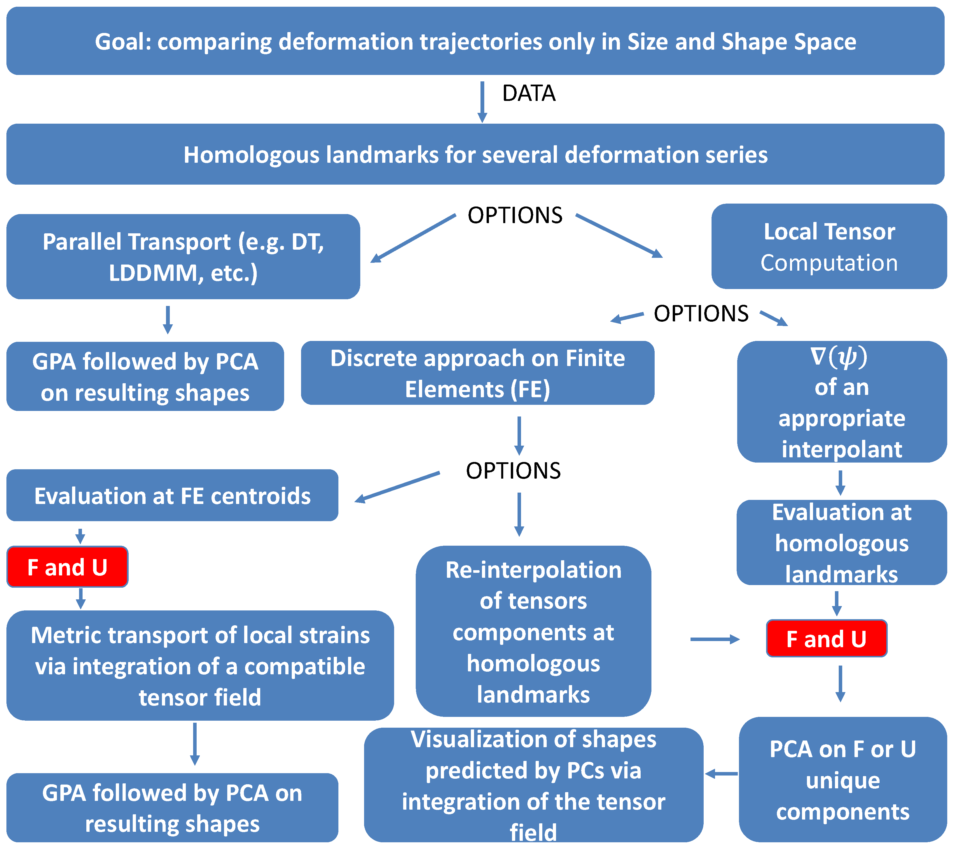
In the summary box of Figure 1 we illustrate main pathways available in order to perform analyses aimed at studying deformative processes only. We related the various options described in the text to the use of tensors in shape analysis.

4. Materials and Methods

4.1. Computational Details

All R code (fully commented) and data (provided as R workspaces) used in the analyses presented in this paper are available as Supplementary Information, ensuring full reproducibility and public accessibility. The functions are included in the R package combin, which is downloadable at the following link: https://figshare.com/articles/software/combin_0_0_0_9000_tar_gz/28737332?file=58130416 and must be installed as a local source using devtools R package [50] by calling the following command line: devtools::install_local(your-path-to-file, upgrade = “never”, force = TRUE) (accessed on 18 October 2025).

This package is undocumented, but the scripts included with this article are fully commented on. This package also contains many functions (some of them very old or just modified/hacked wrappers of some existing functions in other packages used just as ancillary functions) not used for the purposes of this paper. The reader is urged to cite this paper if they want to use the material present in this Supplementary Material in any way. All R scripts are designed to run independently, reproducing all figures presented in the text. They also automatically call and install any required dependencies if missing (note that this process may take some time on a freshly installed R system). R version 4.4.1 or higher is required.

4.2. Strain Tensor Estimation

In the context of MSA, recently, refs. [8,51] presented the use of local strain tensors as

• A tool for interpreting local shape change.
• As a diagnostic criterion to evaluate the goodness of different Parallel Transport methods.

They presented a variety of methods to estimate local tensors $\mathbf{F}$, which can be summarized as follows:

(1)

Discrete Evaluation: this involves using displacement fields at the centroids of predefined finite elements (triangles in both ${\mathbb{R}}^2$ and ${\mathbb{R}}^3$ and tetrahedra in ${\mathbb{R}}^3$) for both undeformed and deformed configurations. The triangulation and tetrahedralization matrices must be “homologous” across different individuals, meaning they should be defined by the same number of elements and identified using the same points (i.e., homologous landmarks + possible Steiner points) indices.

Single elements are defined a priori and are contingent upon the meshing algorithm used for triangulation or tetrahedralization. Creating a sufficiently dense mesh can help mitigate the inherent arbitrariness associated with the triangulation or tetrahedralization structure. This procedure focuses on pure geometric deformation without considering the forces and constraints applied to the body.

Ref. [25] refers to this as the “descriptive finite element,” in contrast to the “constitutive finite element,” which takes into account forces, their directions, and constraints; this approach is proper for CM.

Ref. [51] presented algebraic details for estimating the deformation gradient $\mathbf{F}$ using displacement fields for triangles in both ${\mathbb{R}}^2$ and ${\mathbb{R}}^3$, which will not be reiterated here. The slightly modified workflow for estimating $\mathbf{F}$ between an undeformed tetrahedron X and its deformed state $X^{\prime }$ is as follows:

We calculate the covariant basis vectors ${\mathbf{a}}_1$, ${\mathbf{a}}_2$, and ${\mathbf{a}}_3$ for both X and $X^{\prime }$ as the vector differences between one vertex ${\mathbf{p}}_1$ and the others ${\mathbf{p}}_2$, ${\mathbf{p}}_3$, and ${\mathbf{p}}_4$:

For X we have

$$\begin{array}{cc}\hfill {\mathbf{a}}_1& ={\mathbf{p}}_4-{\mathbf{p}}_1\hfill \end{array}$$

(1)

$$\begin{array}{cc}\hfill {\mathbf{a}}_2& ={\mathbf{p}}_3-{\mathbf{p}}_1\hfill \end{array}$$

(2)

$$\begin{array}{cc}\hfill {\mathbf{a}}_3& ={\mathbf{p}}_2-{\mathbf{p}}_1\hfill \end{array}$$

(3)

For $X^{\prime }$ we have

$$\begin{array}{cc}\hfill {\mathbf{a}}_1^{\prime }& ={\mathbf{p}}_4^{\prime }-{\mathbf{p}}_1^{\prime }\hfill \end{array}$$

(4)

$$\begin{array}{cc}\hfill {\mathbf{a}}_2^{\prime }& ={\mathbf{p}}_3^{\prime }-{\mathbf{p}}_1^{\prime }\hfill \end{array}$$

(5)

$$\begin{array}{cc}\hfill {\mathbf{a}}_3^{\prime }& ={\mathbf{p}}_2^{\prime }-{\mathbf{p}}_1^{\prime }\hfill \end{array}$$

(6)

Next, we can derive the contravariant basis using ${\mathbf{a}}_3$:

$$\begin{array}{cc}\hfill {\mathbf{a}}^1& ={\displaystyle \frac{{\mathbf{a}}_2\times {\mathbf{a}}_3}{{\mathbf{a}}_1·({\mathbf{a}}_2\times {\mathbf{a}}_3)}}\hfill \end{array}$$

(7)

$$\begin{array}{cc}\hfill {\mathbf{a}}^2& ={\displaystyle \frac{{\mathbf{a}}_3\times {\mathbf{a}}_1}{{\mathbf{a}}_1·({\mathbf{a}}_2\times {\mathbf{a}}_3)}}\hfill \end{array}$$

(8)

$$\begin{array}{cc}\hfill {\mathbf{a}}^3& ={\displaystyle \frac{{\mathbf{a}}_1\times {\mathbf{a}}_2}{{\mathbf{a}}_1·({\mathbf{a}}_2\times {\mathbf{a}}_3)}}\hfill \end{array}$$

(9)

The deformation gradient $\mathbf{F}$ is then obtained as

$$\mathbf{F}=({\mathbf{a}}_1^{\prime }\otimes {\mathbf{a}}^1)+({\mathbf{a}}_2^{\prime }\otimes {\mathbf{a}}^2)+({\mathbf{a}}_3^{\prime }\otimes {\mathbf{a}}^3)$$

(10)

where ⊗ denotes the Kronecker product. The $\mathbf{F}$ tensor obtained in this way describes the deformation of the individual element as estimated at its centroid.

(2)

Evaluation of the first gradient $\nabla \left(\psi \right)$ of an appropriate interpolant $\psi$ at desired positions within a body. The choice of the interpolant is completely arbitrary even if some approaches could be more versatile than others (see below). The evaluation points are also an arbitrary choice. Here, they coincide with source homologous landmarks (except for diagnostics made using centroids of finite elements).

Ref. [51] presented algebraic details for the evaluation of $\nabla \left(\psi \right)$ when $\psi$ is represented by the TPS in ${\mathbb{R}}^2$ and ${\mathbb{R}}^3$ and will not be re-proposed here.

Here we add details for the “quadratic trend” (QT) and “cubic trend” (CT) least squares interpolants recently exploited by [39]:

• In ${\mathbb{R}}^2$ the deformation gradient $\mathbf{F}$ is the $2\times 2$ Jacobian matrix $\mathit{J}$

  $$\begin{array}{c}\hfill \mathit{J}(x,y)=\left(\begin{array}{cc}{\displaystyle \frac{\partial {\mathit{\psi }}_1}{\partial x}}& {\displaystyle \frac{\partial {\mathit{\psi }}_1}{\partial y}}\\ {\displaystyle \frac{\partial {\mathit{\psi }}_2}{\partial x}}& {\displaystyle \frac{\partial {\mathit{\psi }}_2}{\partial y}}\end{array}\right)\end{array}$$

  (11)

  In ${\mathbb{R}}^3$ $\mathit{J}$ is the $3\times 3$ matrix

  $$\begin{array}{c}\hfill \mathit{J}(x,y,z)=\left(\begin{array}{ccc}{\displaystyle \frac{\partial {\mathit{\psi }}_1}{\partial x}}& {\displaystyle \frac{\partial {\mathit{\psi }}_1}{\partial y}}& {\displaystyle \frac{\partial {\mathit{\psi }}_1}{\partial z}}\\ {\displaystyle \frac{\partial {\mathit{\psi }}_2}{\partial x}}& {\displaystyle \frac{\partial {\mathit{\psi }}_2}{\partial y}}& {\displaystyle \frac{\partial {\mathit{\psi }}_2}{\partial z}}\\ {\displaystyle \frac{\partial {\mathit{\psi }}_3}{\partial x}}& {\displaystyle \frac{\partial {\mathit{\psi }}_3}{\partial y}}& {\displaystyle \frac{\partial {\mathit{\psi }}_3}{\partial z}}\end{array}\right)\end{array}$$

  (12)
• With $\psi$, a least squares Quadratic Trend regression in ${\mathbb{R}}^2$, we have

  $$\begin{array}{c}\hfill (x^{\prime },y^{\prime })=(a+bx+cy+v{x}^2+sxy+t{y}^2),(d+ex+fy+u{x}^2+vxy+w{y}^2)\end{array}$$

  (13)

  Note: in this case only (QT in ${\mathbb{R}}^2$) we name the coefficients as in [39].

  $$\begin{array}{c}\hfill {\displaystyle \frac{\partial {\mathit{\psi }}_1}{\partial x}}=b+2rx+sy\\ \hfill {\displaystyle \frac{\partial {\mathit{\psi }}_1}{\partial y}}=c+sy+2ty\\ \hfill {\displaystyle \frac{\partial {\mathit{\psi }}_2}{\partial x}}=e+2ux+vy\\ \hfill {\displaystyle \frac{\partial {\mathit{\psi }}_2}{\partial y}}=f+vx+2wy\end{array}$$

  (14)
• With $\psi$, a least squares QT regression in ${\mathbb{R}}^3$, we have

  $$\begin{array}{c}\hfill {(x^{\prime },y^{\prime },z^{\prime })}^T=\left(\begin{array}{c}{a}_0+a_{1}x+a_{2}y+a_{3}z+a_4{x}^2+a_{5}xy+a_{6}xz+a_7{y}^2+a_{8}yz+a_{9}z\\ b_0+b_{1}x+b_{2}y+b_{3}z+b_4{x}^2+b_{5}xy+b_{6}xz+b_7{y}^2+b_{8}yz+b_{9}z\\ c_0+c_{1}x+c_{2}y+c_{3}z+c_4{x}^2+c_{5}xy+c_{6}xz+c_7{y}^2+c_{8}yz+c_{9}z\end{array}\right)\end{array}$$

  (15)

  $$\begin{array}{c}\hfill {\displaystyle \frac{\partial {\mathit{\psi }}_1}{\partial x}}=a_1+2a_{4}x+a_{5}y+a_{6}z\\ \hfill {\displaystyle \frac{\partial {\mathit{\psi }}_1}{\partial y}}=a_2+a_{5}x+2a_{7}y+a_{8}z\\ \hfill {\displaystyle \frac{\partial {\mathit{\psi }}_1}{\partial z}}=a_3+a_{6}x+a_{8}y+2a_{9}z\\ \hfill {\displaystyle \frac{\partial {\mathit{\psi }}_2}{\partial x}}=b_1+2b_{4}x+b_{5}x+b_{6}z\\ \hfill {\displaystyle \frac{\partial {\mathit{\psi }}_2}{\partial y}}=b_2+b_{5}x+2b_{7}y+b_{8}z\\ \hfill {\displaystyle \frac{\partial {\mathit{\psi }}_2}{\partial z}}=b_3+b_{6}x+b_{8}y+2b_{9}z\\ \hfill {\displaystyle \frac{\partial {\mathit{\psi }}_3}{\partial x}}=c_1+2c_{4}x+c_{5}x+c_{6}z\\ \hfill {\displaystyle \frac{\partial {\mathit{\psi }}_3}{\partial y}}=c_2+c_{5}x+2c_{7}y+c_{8}z\\ \hfill {\displaystyle \frac{\partial {\mathit{\psi }}_3}{\partial z}}=c_3+c_{6}x+c_{8}y+2c_{9}z\end{array}$$

  (16)
• With $\psi$, a least squares CT regression in ${\mathbb{R}}^2$, we have:

  $$\begin{array}{c}\hfill {(x^{\prime },y^{\prime })}^T=\left(\begin{array}{c}{a}_0+a_{1}x+a_2{x}^2+a_3{x}^3+a_{4}y+a_{5}xy+a_6{x}^{2}y+a_7{y}^2+a_{8}x{y}^2+a_9{y}^3\\ b_0+b_{1}x+b_2{x}^2+b_3{x}^3+b_{4}y+b_{5}xy+b_6{x}^{2}y+b_7{y}^2+b_{8}x{y}^2+b_9{y}^3\end{array}\right)\end{array}$$

  (17)

  $$\begin{array}{c}\hfill {\displaystyle \frac{\partial {\mathit{\psi }}_1}{\partial x}}=a_1+2a_{2}x+3a_3{x}^2+a_{5}y+2a_{6}xy+a_8{y}^2\\ \hfill {\displaystyle \frac{\partial {\mathit{\psi }}_1}{\partial y}}=a_4+a_{5}x+a_6{x}^2+2a_{7}y+2a_{8}xy+3a_9{y}^2\\ \hfill {\displaystyle \frac{\partial {\mathit{\psi }}_2}{\partial x}}=b_1+2b_{2}x+3b_3{x}^2+b_{5}y+2b_{6}xy+b_8{y}^2\\ \hfill {\displaystyle \frac{\partial {\mathit{\psi }}_2}{\partial y}}=b_4+b_{5}x+b_6{x}^2+2b_{7}y+2b_{8}xy+3b_9{y}^2\end{array}$$

  (18)
• With $\psi$, a least squares CT regression in ${\mathbb{R}}^3$, we have:

  $$\begin{array}{cc}\hfill x^{\prime }=& a_0+a_{1}x+a_2{x}^2+a_3{x}^3+a_{4}y+a_{5}xy+a_6{x}^{2}y+a_7{y}^2+a_{8}x{y}^2+a_9{y}^3+a_{10}z\hfill \\ \hfill +& a_{11}xz+a_{12}{x}^{2}z+a_{13}yz+a_{14}xyz+a_{15}{y}^{2}z+a_{16}{z}^2+a_{17}x{z}^2+a_{18}y{z}^2+a_{19}{z}^3\hfill \\ \hfill y^{\prime }=& b_0+b_{1}x+b_2{x}^2+b_3{x}^3+b_{4}y+b_{5}xy+b_6{x}^{2}y+b_7{y}^2+b_{8}x{y}^2+b_9{y}^3+b_{10}z\hfill \\ \hfill +& b_{11}xz+b_{12}{x}^{2}z+b_{13}yz+b_{14}xyz+b_{15}{y}^{2}z+b_{16}{z}^2+b_{17}x{z}^2+b_{18}y{z}^2+b_{19}{z}^3\hfill \\ \hfill z^{\prime }=& c_0+c_{1}x+c_2{x}^2+c_3{x}^3+c_{4}y+c_{5}xy+c_6{x}^{2}y+c_7{y}^2+c_{8}x{y}^2+c_9{y}^3+c_{10}z\hfill \\ \hfill +& c_{11}xz+c_{12}{x}^{2}z+c_{13}yz+c_{14}xyz+c_{15}{y}^{2}z+c_{16}{z}^2+c_{17}x{z}^2+c_{19}y{z}^2+c_{19}{z}^3\hfill \end{array}$$

  (19)

  $$\begin{array}{cc}\hfill {\displaystyle \frac{\partial {\mathit{\psi }}_1}{\partial x}}=& a_1+2a_{2}x+3a_3{x}^2+a_{5}y+2a_{6}xy+a_8{y}^2+a_{11}z+2a_{12}xz+a_{14}yz+a_{17}{z}^2\hfill \\ \hfill {\displaystyle \frac{\partial {\mathit{\psi }}_1}{\partial y}}=& a_4+a_{5}x+a_6{x}^2+2a_{7}y+2a_{8}xy+3a_9{y}^2+a_{13}z+2a_{15}yz+a_{18}{z}^2\hfill \\ \hfill {\displaystyle \frac{\partial {\mathit{\psi }}_1}{\partial z}}=& a_{10}+a_{11}x+a_{12}{x}^2+a_{13}y+a_{14}xy+a_{15}{y}^2+2a_{16}z+2a_{17}xz+2a_{18}yz+3a_{19}{z}^2\hfill \\ \hfill {\displaystyle \frac{\partial {\mathit{\psi }}_2}{\partial x}}=& b_1+2b_{2}x+3b_3{x}^2+b_{5}y+2b_{6}xy+b_8{y}^2+b_{11}z+2b_{12}xz+b_{14}yz+b_{17}{z}^2\hfill \\ \hfill {\displaystyle \frac{\partial {\mathit{\psi }}_2}{\partial y}}=& b_4+b_{5}x+b_6{x}^2+2b_{7}y+2b_{8}xy+3b_9{y}^2+b_{13}z+2b_{15}yz+b_{18}{z}^2\hfill \\ \hfill {\displaystyle \frac{\partial {\mathit{\psi }}_2}{\partial z}}=& b_{10}+b_{11}x+b_{12}{x}^2+b_{13}y+b_{14}xy+b_{15}{y}^2+2b_{16}z+2b_{17}xz+2b_{18}yz+3b_{19}{z}^2\hfill \\ \hfill {\displaystyle \frac{\partial {\mathit{\psi }}_3}{\partial x}}=& c_1+2c_{3}x+3c_5{x}^2+c_{5}y+2c_{6}xy+c_6{y}^2+c_{11}z+2c_{12}xz+c_{14}yz+c_{17}{z}^2\hfill \\ \hfill {\displaystyle \frac{\partial {\mathit{\psi }}_3}{\partial y}}=& c_4+c_{5}x+c_6{x}^2+2c_{7}y+2c_{8}xy+3c_9{y}^2+c_{13}z+2c_{15}yz+c_{18}{z}^2\hfill \\ \hfill {\displaystyle \frac{\partial {\mathit{\psi }}_3}{\partial z}}=& c_{10}+c_{11}x+c_{12}{x}^2+c_{13}y+c_{14}xy+c_{15}{y}^2+2c_{16}z+2c_{17}xz+2c_{18}yz+3c_{19}{z}^2\hfill \end{array}$$

  (20)

4.3. The Ability to Recover a Priori Assigned Strain Tensors: 2D Simulated Case

The logic behind this simulated case is intentionally circular as it is intended to test how and if methods used to estimate tensors can recover a priori assigned local deformation tensors under explicit expectations of their behavior along longitudinal deformation series. We choose a particular set of toy examples to demonstrate the utility of U or F components when evaluating both local and global features of a deformation. Ref. [52] proposed a series of simulations focused on “distortions” characterized by stress-free morphing, i.e., morphing that occurs without accumulation of elastic energy; this can be realized if and only if the geometric domain to which the field applies is “compatible”.

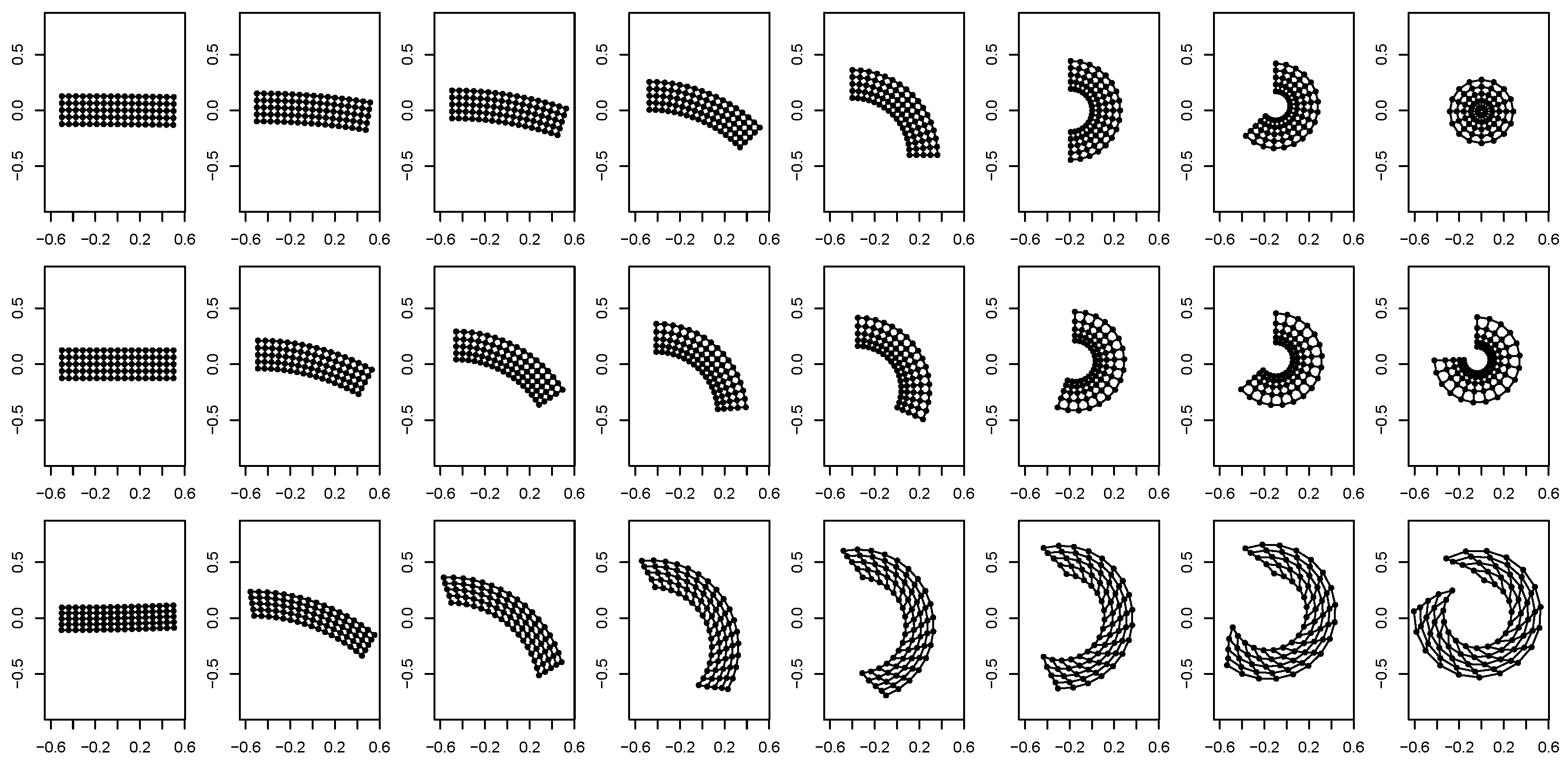
Computationally, this kind of machinery is realized by defining locally appropriate C tensors and integrating $\mathbf{U}=\sqrt{\mathbf{C}}$ over the body domain. As a 2D example, we use a novel modified data version adapted to two dimensions of the example given in Figure 5 of [52] dealing with the bending of a regular parallelepiped as shown in Figure 2.

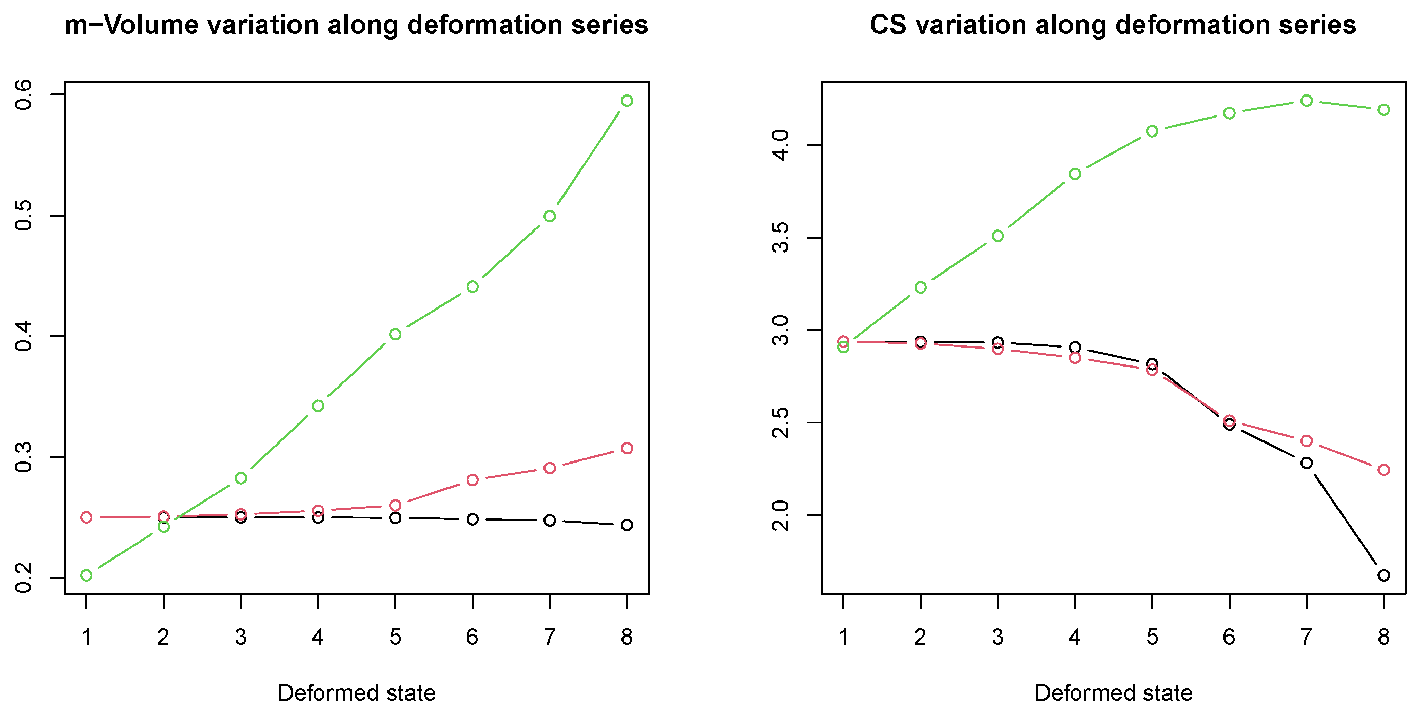
These data are exceptionally valuable, as they provide shape and size deformation series under explicitly a priori assigned strain tensors applied to a compatible geometric domain (see below). As we consider deformations on the x-y plane only, thus ignoring the depth dimension, we use this as a fully two-dimensional example that starts from the (quasi)-regular rectangle (see below). The regular rectangle, composed of 85 landmarks in 2D, is bent in seven deformed forms by tuning, increasing at each step, the curvature radius R of the bending itself. It follows that all forms result from the variation of the sole parameter R. The global deformation can thus be realized by assigning, locally, three different types of (local) U tensors, which are illustrated in Figure 3. Shape changes encoded in these body deformations are relatively large with maximum full Procrustes distance from the source equal to $1.16$, $0.81$ and $0.9$ for the three cases, with $\pi /2$ the maximum allowed. The initial forms are undeformed rectangles, which, due to the parametrization being singular when $R=\infty$, are not perfectly regular. This irregularity is particularly noticeable in the first nematic bending form. Additionally, the initial forms differ in shape from one another; however, this is not a significant issue, as the three series are analyzed separately. The forms belonging to the deformative series experience both shape and size change. It is very interesting to note the completely different behavior of CS and m-Volume (Figure 4). This illustrates how important the quantification of “physical size” could be. We refer the reader to [13] (Section 3: “Two universes for size”) for further consideration on this substantial topic.

Given the very nature of the parameter R in generating these deformation series, we expect, ideally, only one axis explaining 100% of the total variance in a PCA performed on local information extracted by local tensor components.

We motivate here, as illustrated also in the 3D real data example, the use of standard linear PCA. Many other types of non-linear PCA exist that can accommodate the non-linearity of data distributions. Kernel PCA is a classic example [53], while other approaches, such as geodesic PCA [54], can handle shape data lying on Riemannian manifolds. These kinds of PCAs involve several a priori choices, such as the type of kernel or the metric. Our choice here is driven by the need to adopt the most common approach—linear PCA—which is typically used in the majority of shape analyses. Moreover, in the 2D simulated example, we test the ability to recover a single signal (i.e., virtually one principal component) without resorting to non-linear methods.

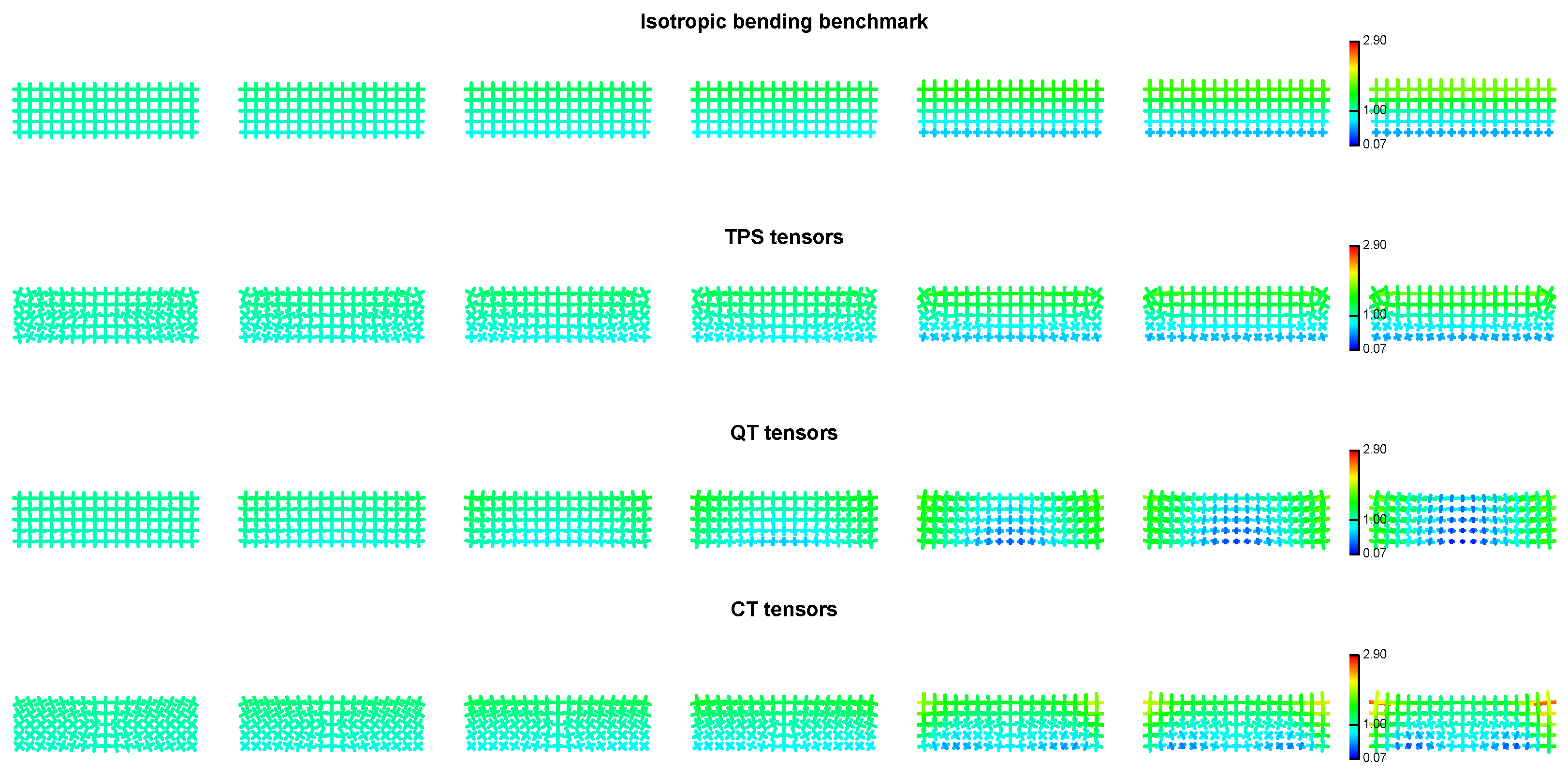
The three types of C strain tensors referring to the three deformed series (“Pure bending”, also called “Normal bending” ), “Isotropic bending”, “Nematic bending”) are the following:

$$\begin{array}{c}\hfill C_{pb}=\left(\begin{array}{cc}{\left(1+\left({\displaystyle \frac{x_3}{R}}\right)\right)}^2& 0\\ 0& 1\end{array}\right)\end{array}$$

(21)

$$\begin{array}{c}\hfill C_{ib}=\left(\begin{array}{cc}{\left(exp\left({\displaystyle \frac{x_3}{R}}\right)\right)}^2& 0\\ 0& 1\end{array}\right)\end{array}$$

(22)

$$\begin{array}{c}\hfill C_{nb}=\left(\begin{array}{cc}{\displaystyle \frac{x_3(1-{\lambda }_{\Vert }^2)}{H}}+{\displaystyle \frac{({\lambda }_{\Vert }^2+1)}{2}}& {\displaystyle \frac{({\lambda }_{\Vert }^2-1)}{2}}\sqrt{1-{\displaystyle \frac{4x_3^2}{H^2}}}\\ {\displaystyle \frac{({\lambda }_{\Vert }^2-1)}{2}}\sqrt{1-{\displaystyle \frac{4x_3^2}{H^2}}}& {\displaystyle \frac{x_3({\lambda }_{\Vert }^2-1)}{H}}+{\displaystyle \frac{({\lambda }_{\Vert }^2+1)}{2}}\end{array}\right)\end{array}$$

(23)

with ${\lambda }_{\Vert }=\sqrt{{\displaystyle \frac{R^2}{H^2+R^2+\sqrt{H^4+4H^2{R}^2}}}}$; $H=\Delta x_3$

With R the bending curvature radius and $x_3$ the value of the y-coordinate in the x-y plane, we use this notation in order to keep it consistent with [52]. With respect to [52], the three formulations have been rewritten in $2\times 2$ format to adapt them to the 2D case and to highlight the sole dependence upon R, given $x_3$. Original (equivalent) definitions ($3\times 3$) are provided by formulas (53) for $C_{\mathrm{pb}}$, (68) for $C_{\mathrm{lb}}$, and (62) for $C_{\mathrm{nb}}$ in [52].

These three parameterized deformations possess some properties allowing particular expectations about tensor features:

• In all three examples, the tensors evaluated at points with the same y-coordinate value on the undeformed shape are constant.
• In “Pure bending”, the local deformation produces only an elongation or a shortening in the x-direction; this means that $\widehat{\lambda }=1$ in the middle of the shape, $\widehat{\lambda }<1$ on the bottom part, and $\widehat{\lambda }>1$ on the upper one.
• In “Isotropic bending”, local deformation maintains, infinitesimally, a local shape; this means that, at any deformed state, we deal exclusively with a spherical local deformation, i.e., ${\lambda }_1/{\lambda }_2=1$ everywhere, and their absolute values increase with the y-coordinate. $det\left(\mathbf{U}\right)=1$ in the middle row, $det\left(\mathbf{U}\right)>1$ on the upper part, and $det\left(\mathbf{U}\right)<1$ on the bottom one. Also, ${\lambda }_1$ and ${\lambda }_2$ absolute values for the same location increase at any deformative step.
• In “Nematic bending”, the shape reflects a nematic elastomer deformation; this means that at each deformative step, ${\lambda }_1/{\lambda }_2=k$, with k constant everywhere at each step and increasing from the first to the last step.

Tensors were computed at landmarks’ locations via TPS, QT, and CT. Source and target were always aligned via OPA (without scaling) before tensor estimation. We performed and compared, for each of the three cases, the following analyses:

• First, we test the ability of the three interpolants we adopt here (TPS, QT and CT) in recovering the assigned U tensors for each step of the three experiments. We did this visually and numerically by evaluating the four above-mentioned expectations. We also directly compared U tensors by computing per-location tensor distance, $d_R=\parallel log\left({\mathbf{S}}_1^{-1/2}{\mathbf{S}}_2{\mathbf{S}}_1^{-1/2}\right)\parallel$, as described by [55] with $S_1$ the assigned tensor and $S_2$ the recovered tensor. The closer $d_R$ is to zero, the better the performance. $d_R$ is the same distance used by [56] (projected on the space of the first few PC scores) in principal coordinate analysis performed on the pairwise $d_R$ distance matrix. The authors of [57] report the same Riemannian distance before proposing their Log-Euclidean transformation on tensors. U tensors’ unique components (3 in ${\mathbb{R}}^2$, 6 in ${\mathbb{R}}^3$) were assembled in a single row for each individual, and on the resulting matrix, we performed an ordination analysis. Using F requires the use all tensor components (4 in ${\mathbb{R}}^2$, 9 in ${\mathbb{R}}^3$). Given n individuals and k tensors, the dimensionality of the matrix of U tensors subjected to PCA is $n\times (k\times 3)$ in ${\mathbb{R}}^2$, $n\times (k\times 6)$ in ${\mathbb{R}}^3$, while for F tensors is $n\times (k\times 4)$ in ${\mathbb{R}}^2$ and $n\times (k\times 9)$ in ${\mathbb{R}}^3$.
• The space of tensors: following [57], U tensors, symmetric, positive-definite matrices, are a specific class of covariance matrices. As noted in the Section 1, they are used in DTI to construct a tensor field, which must often be regularized due to noise inherent in tensor estimation. This regularization is typically performed using non-linear Riemannian metrics. Ref. [57] propose Log-Euclidean transformation followed by exponential map on tensors. This circumvents the above-mentioned issues. Here, we propose to input tensor components into PCA, a Euclidean-linear ordination method. A potential concern is that PCA’s centering step, based on the Euclidean mean, might not be appropriate because the Euclidean mean could deviate significantly from the actual Riemannian (Frechet) mean. However, we argue that in the case of homologous landmark configurations, noise in the deformation mapping is considerably smaller than in typical DTI applications. To empirically assess this assumption, we conduct a direct comparison between the per-location Frechet tensor’s mean vs. Euclidean mean computed across the eight configurations (the undeformed + the seven deformed steps) for the three bending cases. The two means consist of two sets of 85 tensors, each representing one of the two types. We compare these two sets using (i) the ratio between tensor determinants (we expect values $<1$ as it is well known that there is a certain amount of the “swelling” effect in the Euclidean calculus when applied to tensors [57]) and (ii) the Riemannian distance $d_R$ between pairs of homologous tensors. For pure and isotropic bending, a paired Wilcoxon test, coupled with Cohen’s effect size, was performed; for the nematic bending, the determinant is constant, and we limit to the qualitative observation of their ratio. If these diagnostics indicate small differences and small variance, we can reasonably justify the use of the Euclidean mean in this context. We also advocate that, given the very large deformation present in this simulated experiment, the real example (see below), characterized by a maximum Procrustes distance value of 0.37 in pairwise comparisons, will be even less affected by the Euclidean approximation in PCA centering step.
• GPA in SSS followed by PCA on displacements from the first individual.
• PCA on U components computed from the first shape in SSS (TPS, QT and CT).
• PCA on F components computed from the first shape in SSS (TPS, QT and CT).
• Usual GPA in SSS followed by PCA.
• PCA on U components computed from the GPA mean shape in SSS (TPS only).
• PCA on F components computed from the GPA mean shape in SSS (TPS only).
• We visualized predictions of QT and CT for comparison with the original shapes.
• We also visualized $\mathbf{v}$ plotted on source shapes in order to evaluate the behavior of local tensors.
• We computed ${\lambda }_1/{\lambda }_2$ ratio for all tensors (TPS, QT and CT) and plotted their density distribution together with the expected value computed upon the benchmark tensors.

Points 7 and 8 are included to compare PCA on tensors with the usual approach of performing GPA followed by PCA, where displacements are computed from the sample mean.

4.4. Moving to Reality: The 3D Case of Hominidae Skull

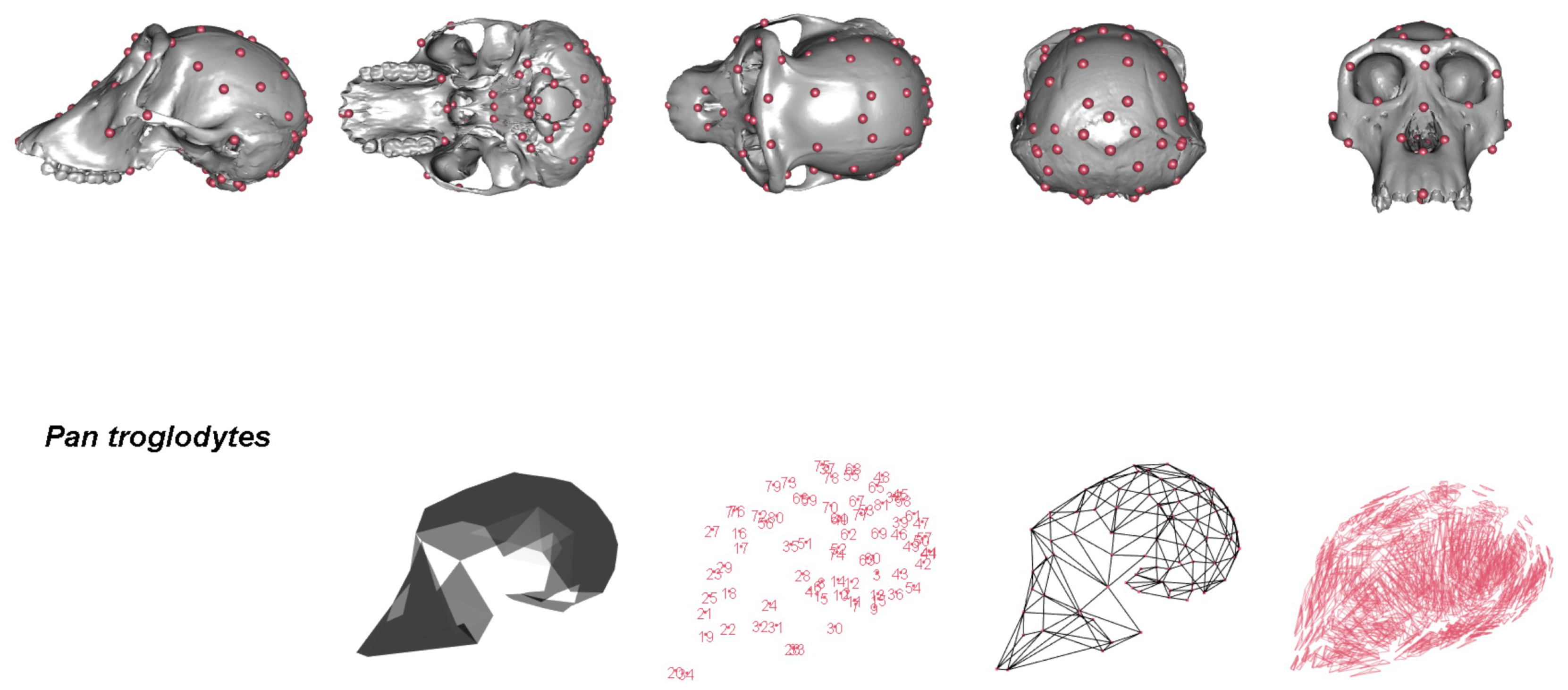
We present here for the first time an unpublished 3D dataset representing an upgrade of that published in [58]. We focus on the crandial anatomy of the hominoids Gorilla gorilla, Homo sapiens, Pan troglodytes, and Pongo pygmaeus. We updated the dataset of these four species in terms of sample size (76 individuals), ontogenetic stage (

Table 2. Sample size for each species at each dental stage. Sexes merged here.

	Stage 1	Stage 2	Stage 3	Stage 4	Stage 5	Stage 6
Gorilla gorilla	0	0	1	5	4	20
Homo sapiens	2	4	6	3	1	19
Pan troglodytes	0	3	8	9	2	21
Pongo pygmaeus	0	0	1	5	7	4

and

Table 3. Ages (in days) corresponding to the achievement of dental stages. Corresponding literature is also indicated. In case of a range, we attributed the mean value.

Dental Stages	1	2	3	4	5	6	Key References
Gorilla gorilla	0–42	42	360	1280	2470	4161	[59] (mean, sexes combined); [60]
Homo sapiens	0–175	175	840	2303	4550	7482	[59] (mean, sexes combined)
Pan troglodytes	0–91	91	360	1210	2470	4130	[59] (mean, sexes combined); [60]
Pongo pygmaeus	0–133	133	385	1277	1825	3650	[61]; [60]

), and landmarking (Figure 5) by adding the neurocranium to the face-base configuration formerly published in [58]. The final 81-landmark configuration also includes surface semilandmarks.

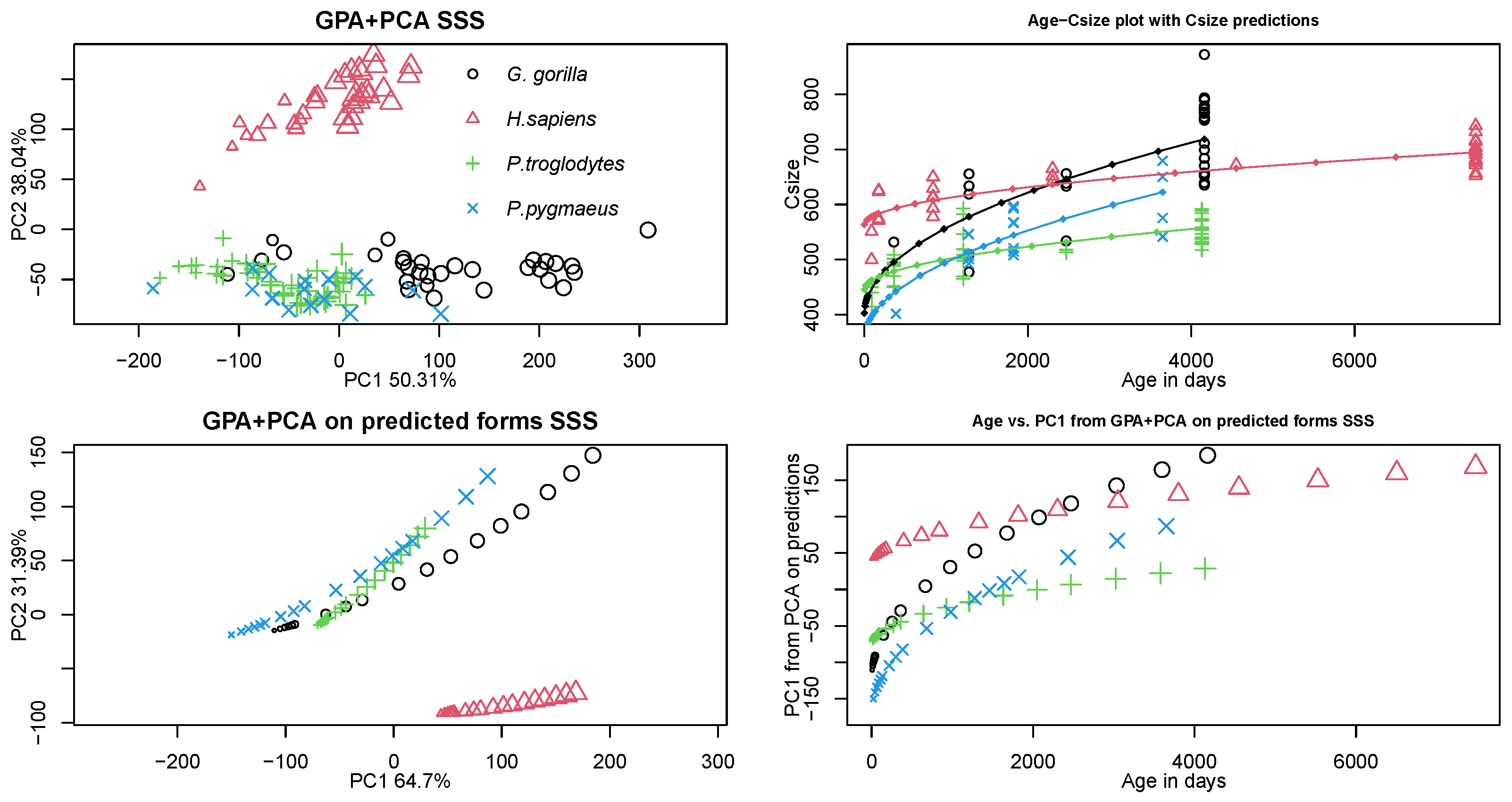
We choose to work with forms predicted by age computed according to the linear regression of GPA-aligned shapes (scaled at unit CS) regressed against the square root of age (in order to manage prediction at age = 0, i.e., newborn), remultiplied with size predicted at the same age values after regressing size against the square root of age. Thus, we refer to “forms predicted in SSS” as the forms obtained via the above-mentioned procedure. This differs substantially by simply regressing non-scaled forms against age. The prediction age vector was set, for each species separately, by adding age 0 to the six dental ages. Using these seven ages, we interleave between consecutive values two equally spaced values. Age-0 is set as the youngest prediction age (

Table 4. Per-species prediction age-vectors (in days).

Gorilla gorilla	0	7	14	21	28	35	42	148	254	360	667	973	1280	1677	2073	2470	3034	3597	4161
Homo sapiens	0	29	58	88	17	146	175	397	618	840	1328	1815	2303	3052	3801	4550	5527	6505	7482
Pan troglodytes	0	15	30	46	61	76	91	81	270	360	643	927	1210	1630	2050	2470	3023	3577	4130
Pongo pygmaeus	0	22	44	67	89	111	133	217	301	385	682	980	1277	1460	1642	1825	2433	3042	3650

). The final prediction age vectors consist of 19 age values for each species that could be considered approximately ontogenetically homologous among the four species.

Of course, a certain amount of approximation is present in this aging procedure (for some species, we were forced to extrapolate), but we believe it can be consistently used for comparison among different species that are very dissimilar in terms of shape, size, and form-change rates. Moreover, given the methodological aim of the present paper, we believe that small deviations from the above-mentioned prediction procedure should not affect the main interpretation and conclusions, as the predicted shapes (regardless of the chosen prediction strategy) serve merely as the starting data for all analyses presented here. A similar approach was used in [62], where some caveats and limitations for this method were exposed. Thus, the expression “homologous ages” or “homologous times” must always be intended as “homologous” in terms of ages corresponding to the same dental eruption class. The entire procedure was performed for each species separately in the same mode. All individuals belonging to dental stage six received the same species-specific age value, i.e., that of the acquisition of complete maturity; while it is certainly true that additional morphological changes occur in cranial morphology after dental maturity-age, we judge them to be negligible in comparison to those occurring during the entire post-natal ontogenetic process.

We performed the following analyses on per-species predictions:

• Usual GPA in SSS followed by a PCA.
• DT in SSS followed by PCA.
• PCA on U components computed from the youngest prediction in SSS (TPS, QT, and CT).
• PCA on F components computed from the youngest prediction in SSS (TPS, QT, and CT).
• PCA on U components computed from the GPA mean shape in SSS (TPS only).
• PCA on F components computed from the GPA mean shape in SSS (TPS only).
• We compared tensors (using the $d_{\mathrm{R}}$ distance) computed in a discrete manner on finite elements of triangles and tetrahedra with those computed at element centroids via TPS, QT, and CT, based on the deformations observed between the youngest (as sources) and all other per-species predictions (as targets). We also add to these comparisons the tensors estimated on data transported according to the DT Parallel Transport, as we judge relevant the contrast between individual per-group tensor’s estimation and that performed on transported data; for transported data, both TPS and discrete modalities were used. While tensors derived from finite elements cannot be considered a true analytical benchmark, we believe that, given the same triangulation or tetrahedralization structure used for all forms, the discrete approach provides a neutral way to assess the reliability/versatility of different interpolants. Triangulation and tetrahedralization are shown in Figure 5 (bottom-right); tetrahedralization was obtained using “alphashapes3d” R package [63]. We anticipate that tetrahedra so obtained are not quality checked and some quasi-degenerate element exist (Figure 5); however, they are not used for biological interpretation here but just for comparison among the different interpolation methods; there are some approaches for constraining tetrahedralization in a manner more adherent to the actual morphology (e.g., using triangulation as constraint), but these are outside the scope of the present paper. In both cases, the two connectivity matrices were retained for all comparisons. The same approach (using quality-checked triangulation) was employed in [8,20] to evaluate the accuracy of different PT methods. We chose both triangles and tetrahedra due to their distinct physical interpretations: triangles describe plane-surface deformations, while tetrahedra capture changes in full volumetric local domains. The procedures for projecting a full rank $3\times 3$ F tensor, evaluated at a triangle face centroid in ${\mathbb{R}}^3$ (via the discrete way or an interpolant either) onto the plane containing the face and for reducing the resulting singular $3\times 3$ tensor to a non-singular $2\times 2$ tensor via a change of basis are detailed in [51].
• We also visualized U (on sources) and F (on targets) tensors evaluated at homologous landmarks as ellipsoids using TPS, QT and CT in order to compare their different abilities in explaining growth processes. Youngest–oldest comparison was chosen for this purpose, and some primatological considerations were made.

Points 5 and 6 are included to compare PCA on tensors with the usual approach of performing GPA followed by PCA, where displacements are computed from the sample mean. We think that, biologically speaking, choosing the template as the mean of shapes predicted at the youngest homologous ages is the most reasonable option, as it allows us to follow entirely the direction of shape change due to the growth process.

5. Results

5.1. Two-Dimensional Simulated Case

We state, without illustrating this result, that, for the three bending cases, a PCA performed on the unique components of assigned U tensors returns, as expected, only one axis explaining 100% of the total variance in pure and nematic bending with points distributed on perfectly horizontal trajectories in a PC1-PC2 plot (with 0% of variance explained by PC2), while for the isotropic bending, we see the PC1 explaining 99.64% of total variance and 0.34% explained by PC2.

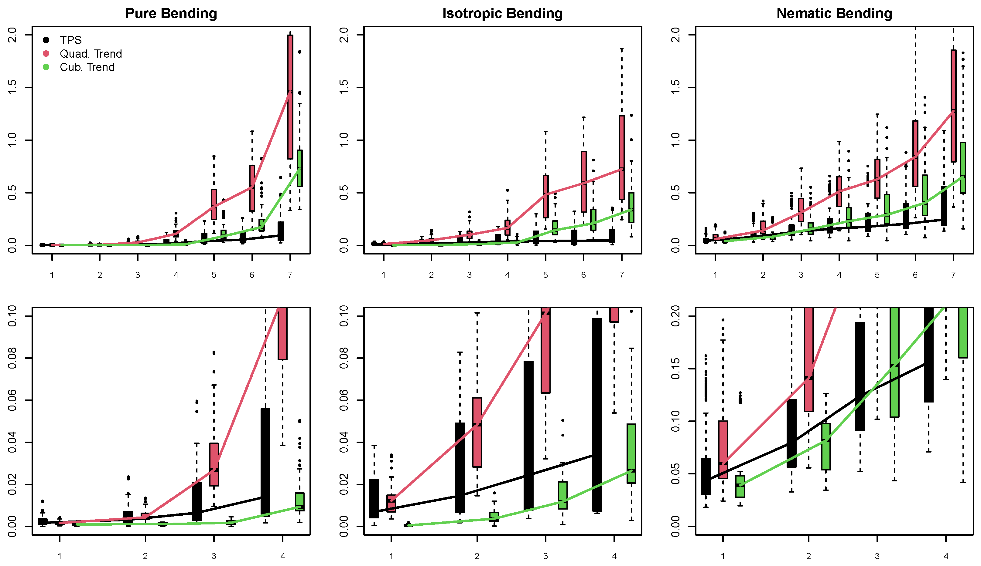
Figure 6 shows the $d_R$ distance between assigned benchmark U tensors and the three interpolants used to recover them locally. TPS scores below QT and CT, with CT better than QT mainly at the most deformed states; a closer look at the first four states reveals that for small deformations, CT performs better than TPS; however, $d_R$ values are very small there. When the degree of deformation is augmented, the differences in $d_R$, among the three methods, become much larger with a TPS that maintains relatively small $d_R$ values with respect to QT and CT.

Supplementary Table S1 reports paired Wilcoxon test and effect sizes, as Vargha and Delaney’s A, for all deformational steps.

As for the comparison between the Euclidean and Fréchet means we obtained, in pure and isotropic bending, significant paired Wilcoxon test due to the very small variability (the distributions are highly non-normal) of determinants (in pure bending median determinant ratio between Fréchet and Euclidean means: 0.990 with a coefficient of variation equal to 0.034; isotropic bending: 0.987 with a coefficient of variation equal to 0.017); however, Cohen’s d is dramatically low (−0.098 and −0.040 respectively), indicating very small differences. The ratio between determinants using the two means in the nematic bending is 0.94. $d_R$ median values were 0.017, 0.034, and 0.060 for pure, isotropic, and nematic bending, respectively, comparable to $d_R$ between benchmark tensors and the interpolants at the first deformed states. All these results suggest a reasonable adequacy of the Euclidean mean in PCA centering.

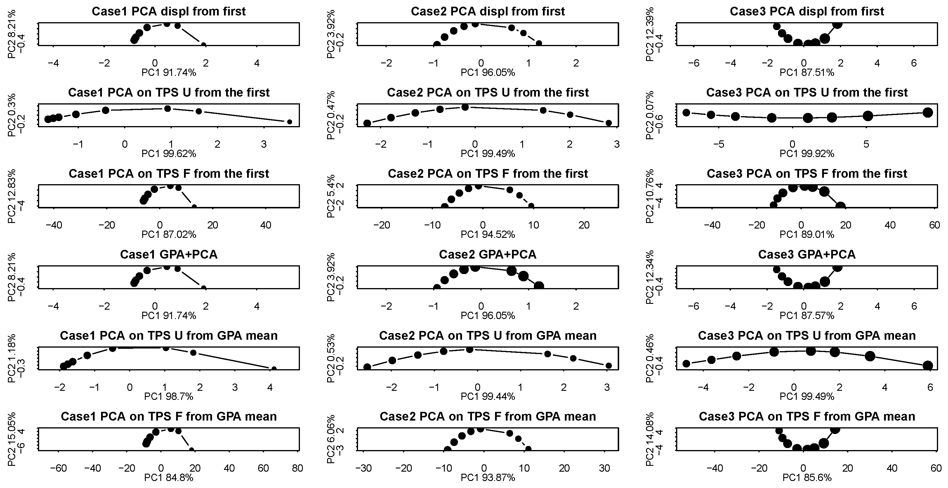
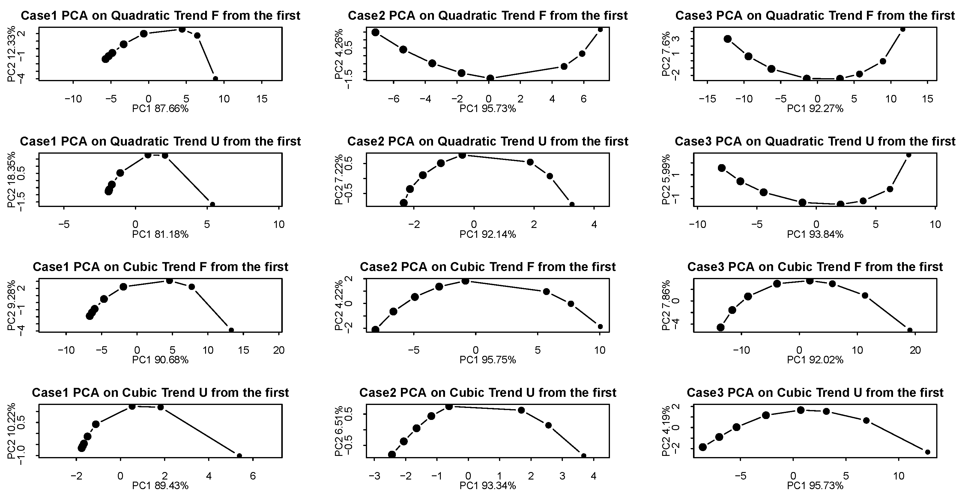
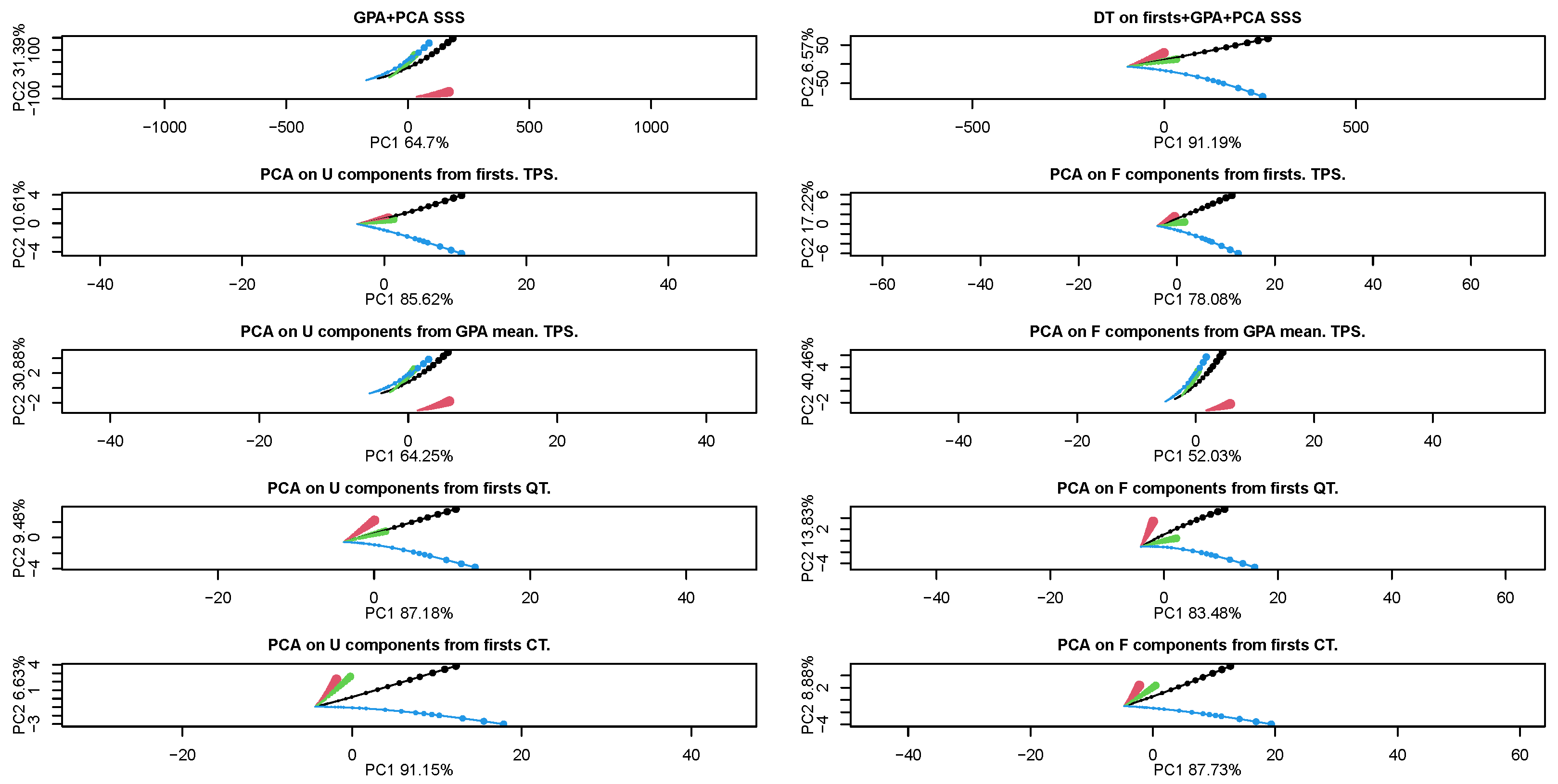
Figure 7 and Figure 8 show the PCA performed on tensor components and displacements after GPA. The PCA conducted on U, recovered via TPS using the first individual of each series as source, closely approaches 100% of the total variance concentrated in the PC1 axis (ranging from 99.5% to 99.9%). A virtually identical pattern is observed when the source is set as the GPA mean. In contrast, using displacements or F tensor components does not return the same performance, resulting in a “parabolic” trajectory with less variance explained by PC1 (ranging from 85% to 95%). This behavior of F is expected, as F also encodes local infinitesimal rotation, and the bent shapes were obtained using U, not F (see discussion). Displacements exhibit patterns very similar to those of F.

In [64], there are further considerations about parabolic behavior in PCA related to trend or random walk models. In particular, it was noted that although in a PCA, PC1 and PC2 are orthogonal by construction, in some cases, they are far from being uncorrelated/independent.

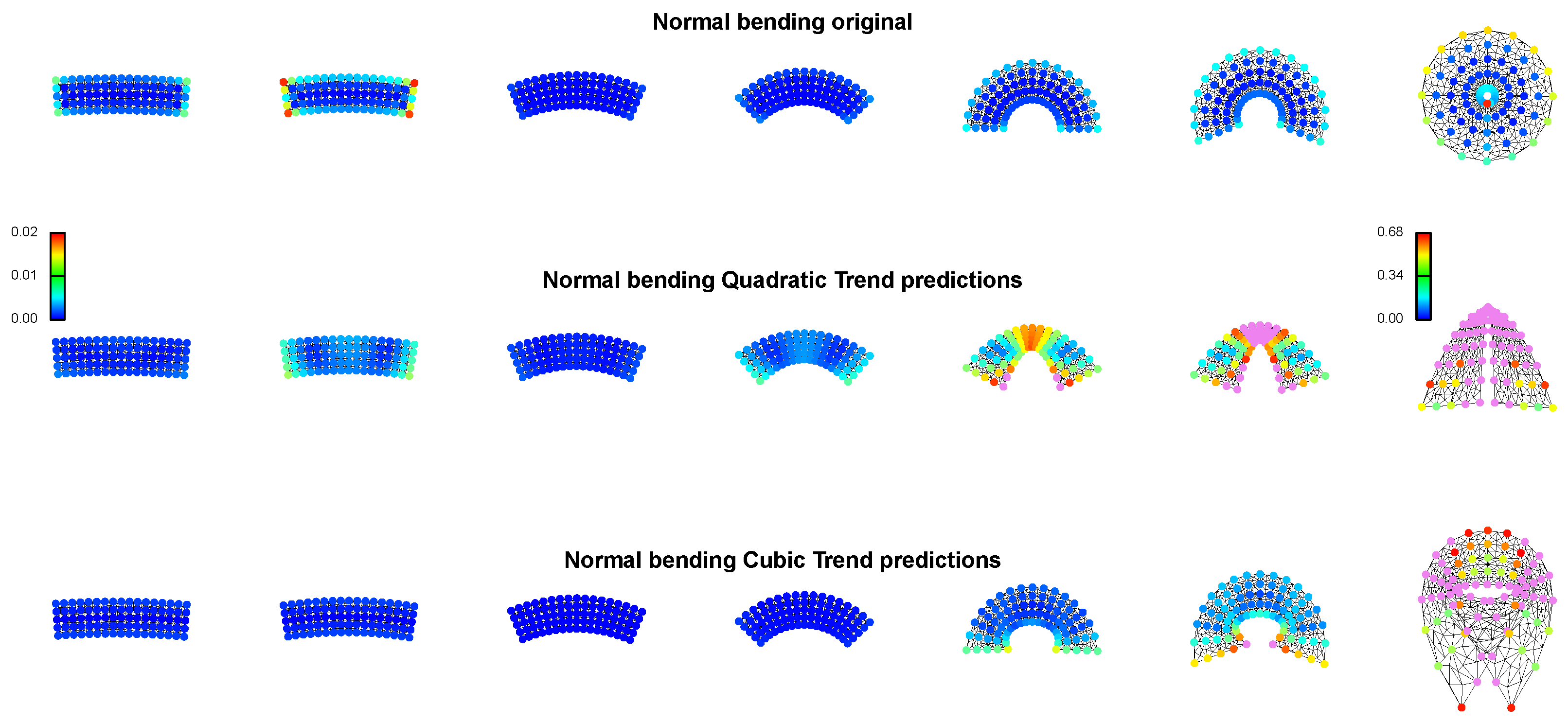
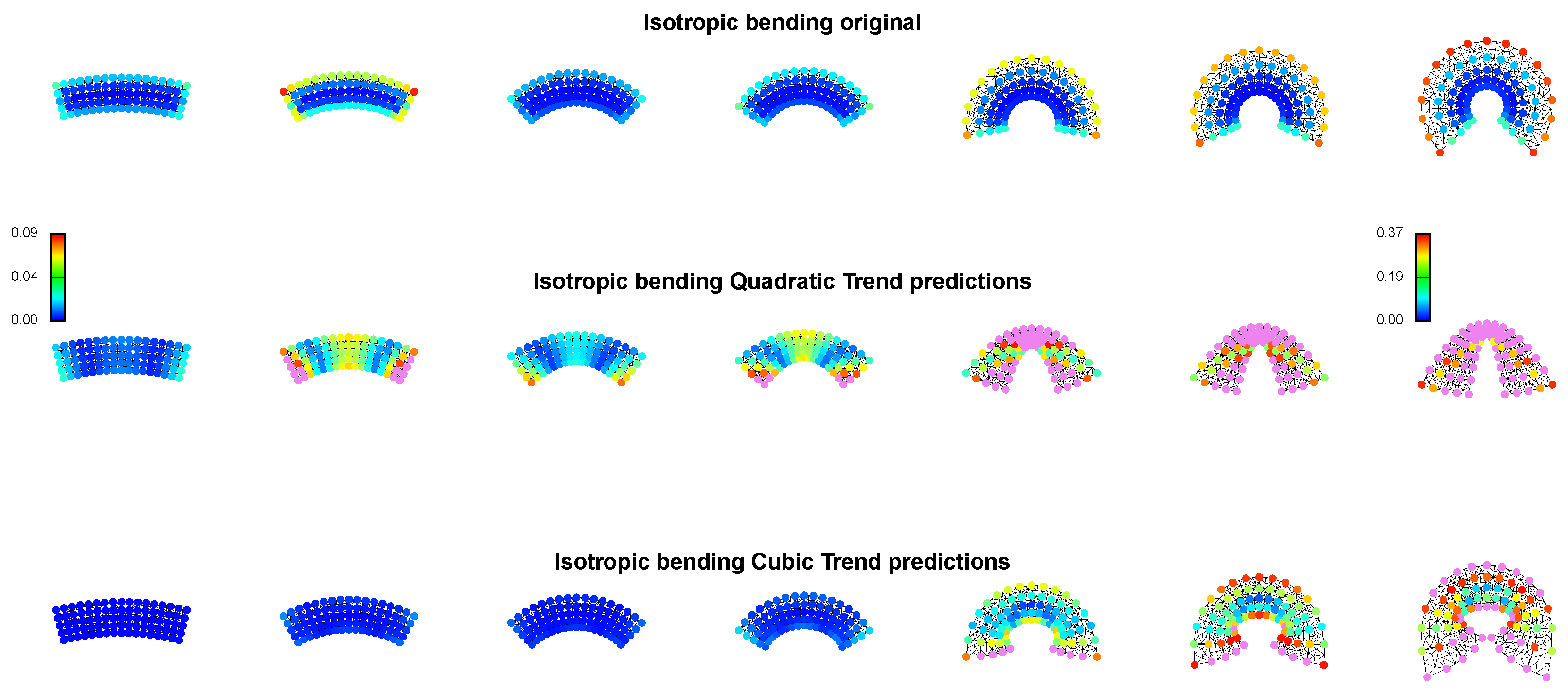
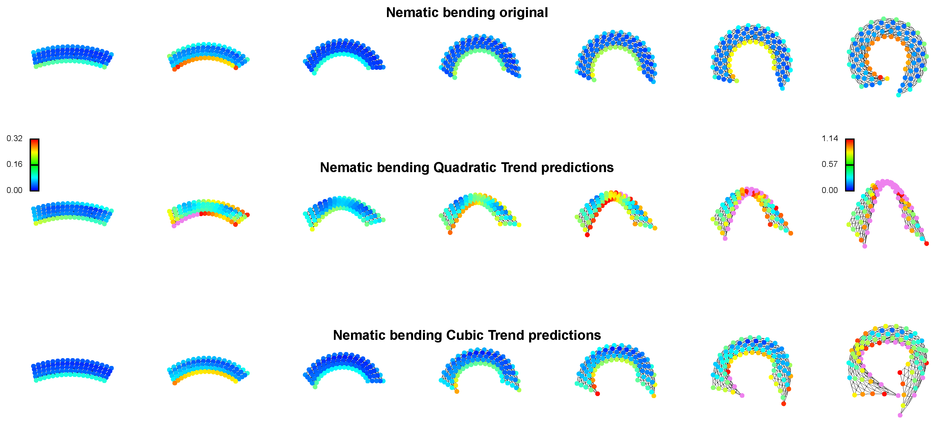
QT and CT do not achieve a full concentration of variance in PC1. In fact, the first three to four individuals follow a nearly linear trajectory, which then visibly bends, creating a curved global path along PC2. This can be explained by the fact that, when deformations become particularly large, QT and CT fail to accurately predict the actual target, as illustrated in Figure 9, Figure 10 and Figure 11, making the recovery of local deformation tensors particularly challenging. There, we visualize landmarks colored according to $d_R$ distance, equipped with a triangular deformation grid limited to the body-only, in order to show the presence or absence of foldings on the body domain. Folding is visible in the last deformed state for CT interpolation in the pure bending case. This is due to the fundamental differences between TPSs, which minimize the bending energy quantifying the smoothness of the deformation by integrating the squared second-order partial derivatives over the entire domain while enforcing an exact interpolation through the target points (thus resulting in zero interpolation error) and least-squares approaches, which instead minimize the sum of squared differences between observed and predicted values (see [39] for further discussion).

Figure 9, Figure 10 and Figure 11 convey an important message related to these specific bending scenarios: they help explain why, in Figure 6, CT appears more robust than TPS in recovering assigned tensors during the first three or four deformed states. As shown in Figure 9, Figure 10 and Figure 11, TPS is affected by a reduced performance primarily at landmarks located along the boundaries of the body. The bending patterns used in this study include quadratic and cubic components in their displacement fields as a consequence of C tensor definitions. CT benefits from this type of spatial variation, leading to better performance in the early deformed states. When the deformation increases, however, CT predictions deviate substantially, preventing accurate recovery of the assigned tensors—this is also evident in the body-only triangular deformation grids (chosen in order to prevent excessive folding of the grid itself outside the body). TPS does not show this issue: although its requirement of decaying to zero outside the body causes reduced performance in the initial deformation steps, TPS’s zero error at predictions properly ensures stable adherence to the assigned tensors even at highly deformed states. Thus, CT performs well in the initial deformation states largely due to the fortuitous presence of quadratic–cubic components in the displacement fields, which align with the formal structure implied by the assigned tensors. Also, differences in $d_R$ distance between TPS and CT at early stages in favor of CT are very small if compared to that at the last stages in favor of TPS.

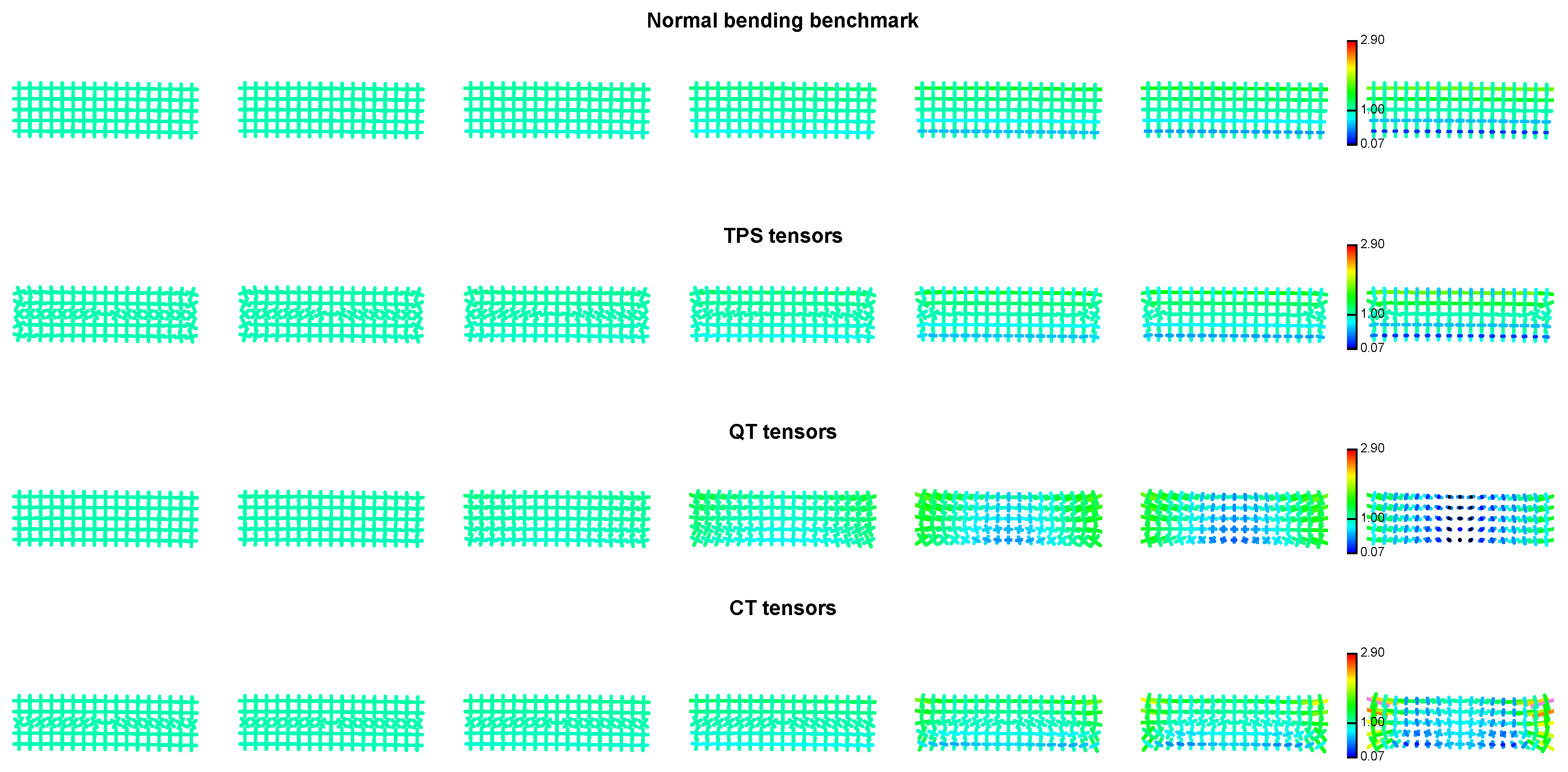
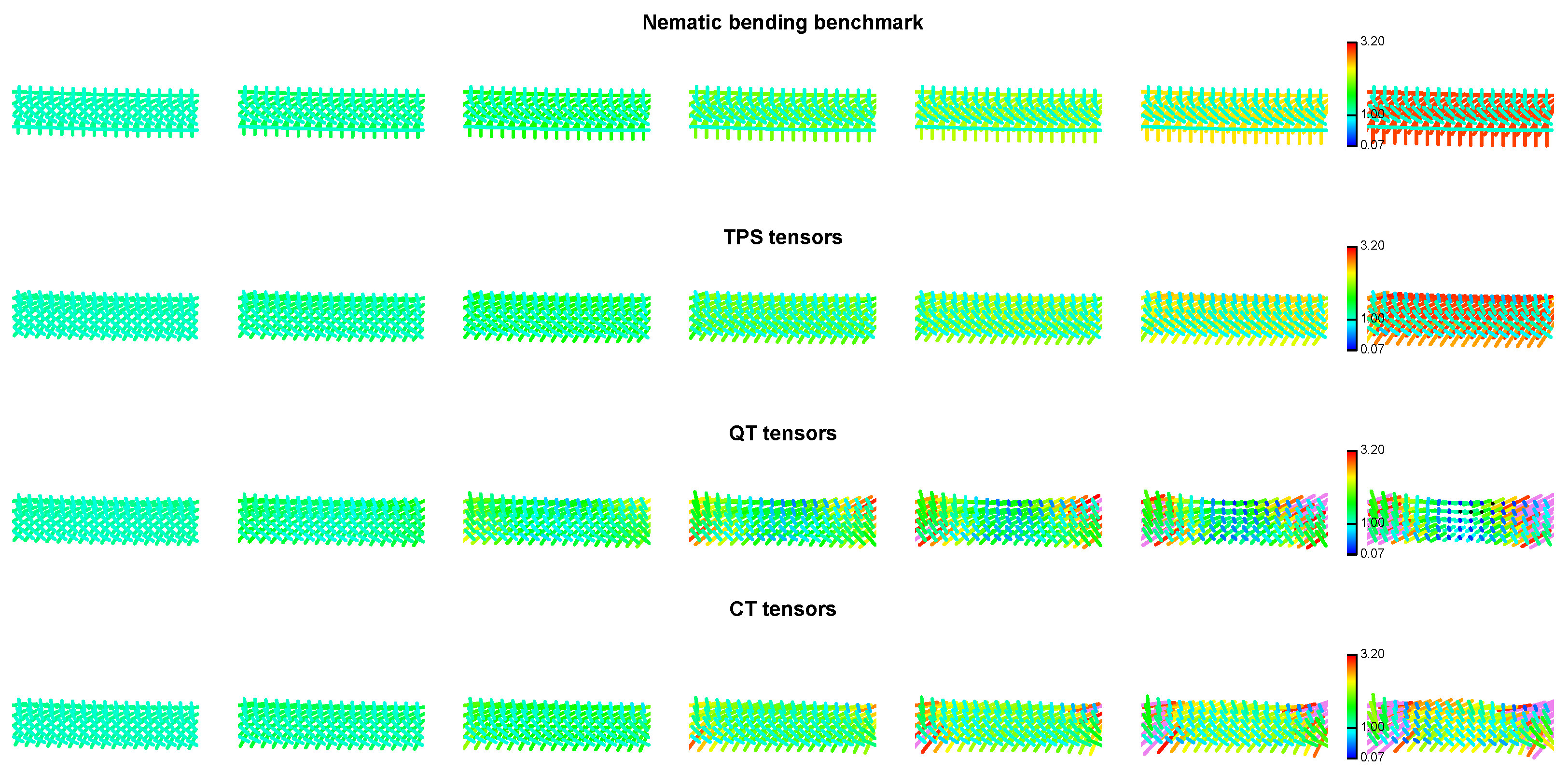
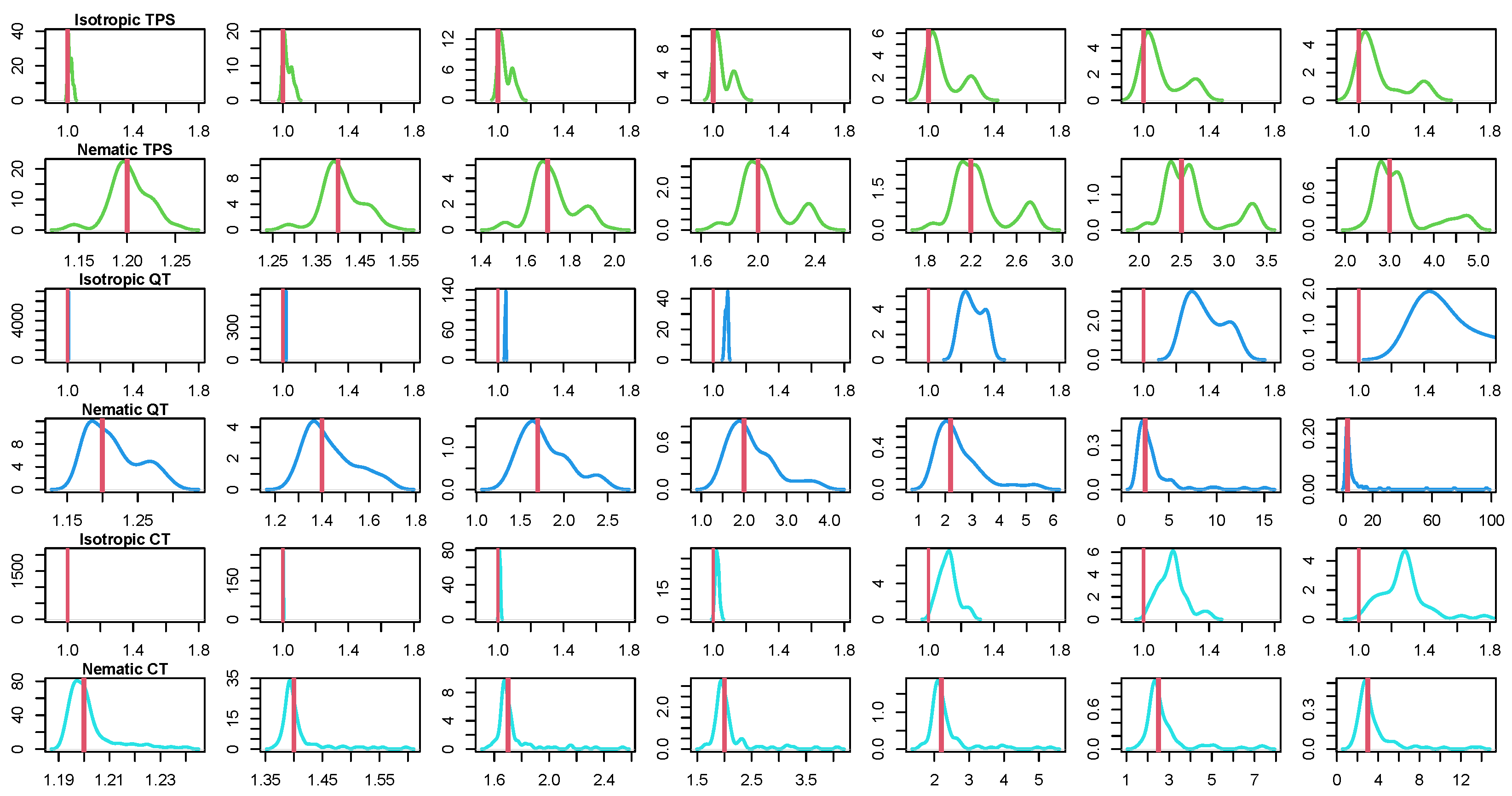
The behavior of PCA is not sufficient to account for the physical meaning of local tensors and their adherence to the theoretical expectations listed in the Section 4. For this purpose, we present in Figure 12, Figure 13, Figure 14 and Figure 15 the assigned U tensor’s $v$, as well as those recovered via TPS, QT, and CT, respectively, plotted on the source forms according to corresponding deformed states. For recovered $v$, we also plot the expected value of the ${\lambda }_1/{\lambda }_2$ ratio for isotropic and nematic bending contrasted with the density distributions of ${\lambda }_1/{\lambda }_2$ of recovered tensors. Comparing TPS, QT, and CT, we can observe that $v$ from TPS better adheres not only to the benchmark ones in terms of directions and $\lambda$ magnitudes but also to the expectations of the ${\lambda }_1/{\lambda }_2$ ratio for the isotropic and nematic bending cases. QT and CT ${\lambda }_1/{\lambda }_2$ density distribution in the nematic bending case is dispersed around the expected value, but with a much larger spreading with respect to TPS. Moreover, QT and CT $v$ show incorrect behavior for the most deformed cases, which is not coherent with assigned deformations: when it is expected that $\lambda \gg 1$, it happens to find $\lambda \ll 1$, as suggested by the color scale that indicates $\lambda$ magnitude.

It must be said that for the first three deformed states QT and CT perform rather well in a manner that is comparable to TPS (see also the prediction plots). As these bending cases are very challenging in terms of form (and shape) differences with respect to sources, the least squares trends struggle to accurately recover the tensors in the most deformed targets.

The decision to plot $v$ on the source rather than $\mathbf{F}v$ on the targets (the difference is the local rotation) is based on the guess that, in these particular cases where a benchmark is available (differently from real biological data), the tensor’s behavior is more comparable when visualized in the undeformed state, as the predictions of the three interpolants are different.

5.2. Real Cases: Primate Skull

Figure 16 shows preliminary results on primate skull data. As stated in the Section 4, this illustration refers to SSS only. The top-right and bottom-right panels show the relationship between age vs. CS (both observed and predicted values) and age vs. PC1 of GPA in SSS, followed by a PCA on predicted forms, respectively. Forms predicted at homologous ages were obtained according to the procedure described in the Section 4.

Looking at Figure 16 there are several considerations that could be made relatively to numerous aspects of ontogenetic allometry and heterochrony in Hominidae previously investigated by many other authors ([62,65], among others). For example, the smallest shape and size change in the cranial anatomy of Homo sapiens with respect to other species during development is particularly manifest. This leads to the pedomorphic morphology shown by human adults. Nevertheless, from here forward, we will focus on the methodological results coming from the different procedures described in this paper, in particular, on those derived from the evaluation of PCA performed on local tensor components. Figure 17 shows the entire battery of PCA results upon analyses performed on predicted forms. We consider the comparison between DT and PCA on tensor components particularly relevant. DT has been shown to be a highly robust method [8,20] and can be reasonably adopted as a reference for evaluating the ability of tensors recovered at landmark locations to convey meaningful insights into relative deformational evolution across different longitudinal series when their components are used in ordination analyses.

As stated in the Section 4, tensors relative to a reference (considered as a collection of identity matrices) in a deformation series represent “intrinsic” features of local positions and can be effectively viewed as a tool for “comparing” deformations observed in different bodies from their group-specific references, without relying on a Riemannian connection or metric. A possible computational weakness of this approach could be represented by the fact that, while it is possible to predict tensors explained by some principal component axis values (typically at positive or negative extremes), if one wants to visualize the corresponding forms/shapes deformed with respect to a template, there is the need to integrate tensors over a geometric domain of the template. This procedure, although previously proposed in [16,17], has not been implemented here. It is relatively complex and subject to compatibility restrictions imposed by individual-specific geometric domains [15,16] and does not guarantee convergence in all cases. Approximate approaches do exist, and implementing them for real-world applications remains an area for further investigation.

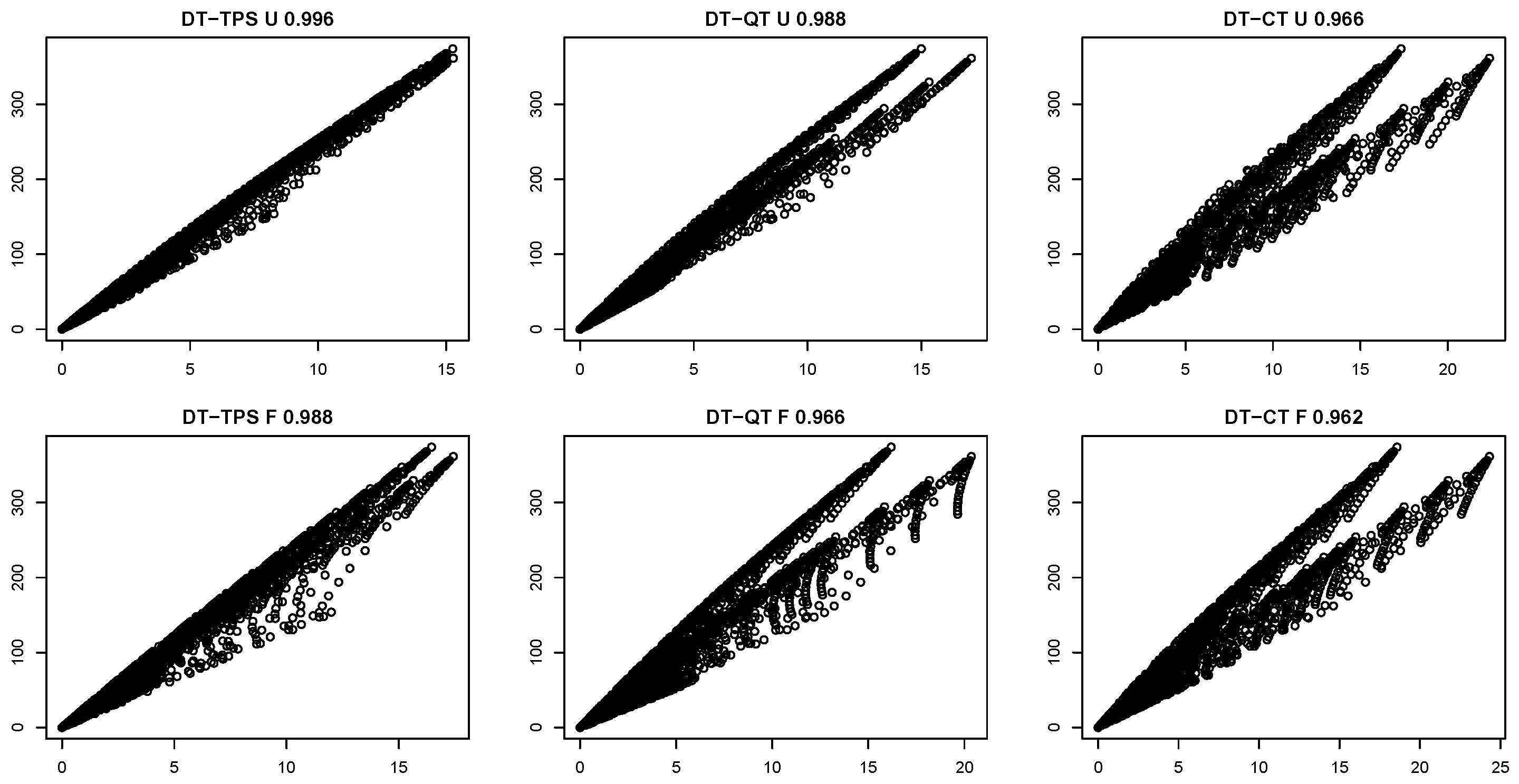
Results of PCA performed on U components derived with TPS highly resemble those performed on transported data according to DT: H. sapiens sets slightly apart from the other species, with P. pygmaeus evidently divergent from P. troglodytes and G. gorilla. As the use of recovered tensors is proposed here as an additional possibility to input local features (i.e., tensor’s components) in ordination analyses, we show in Figure 18 the correlation between PC scores of PCA performed on DT data and the correlations coming from PCA performed on tensor’s components recovered via TPS, QT, and CT. This correlation is performed on pairwise Euclidean distance matrix values computed among (all) scores of the two methods that are contrasted.

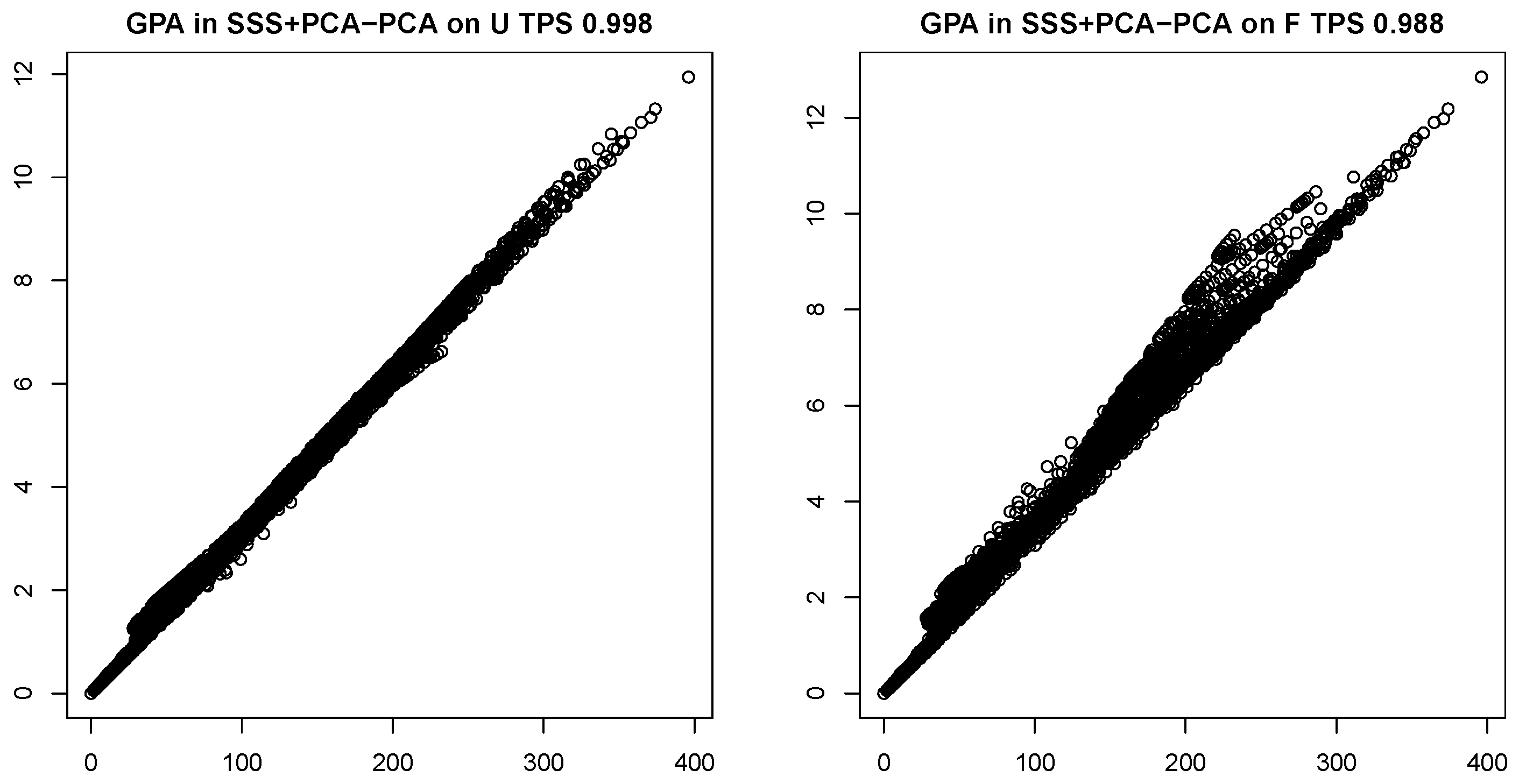
TPS presents the highest correlation values for both U and F analyses with U better correlated than F. QT and CT correlations are not much smaller but the data appear considerably more scattered. We show also in Figure 19 the correlations between PC scores coming from GPA in SSS followed by PCA and those coming from PCA performed on U and F components using the GPA mean as a reference. Both U and F correlate very well with the usual evaluation scores performed on predictions subjected to GPA in SSS with F slightly less correlated.

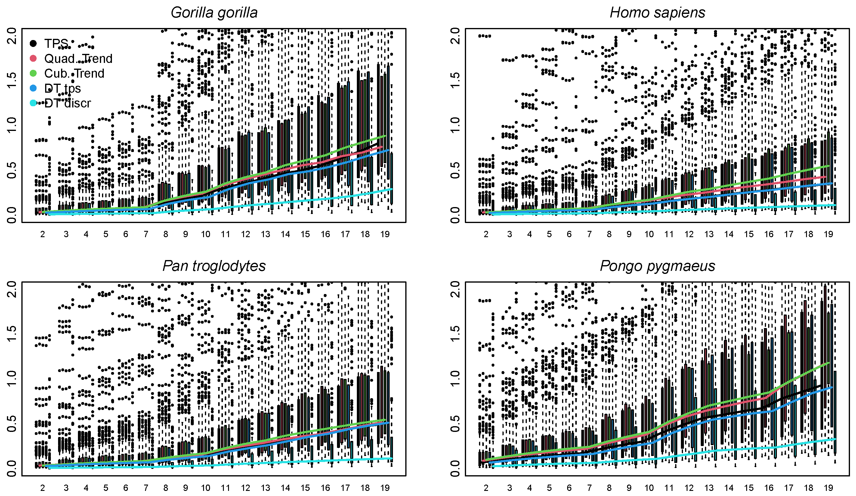
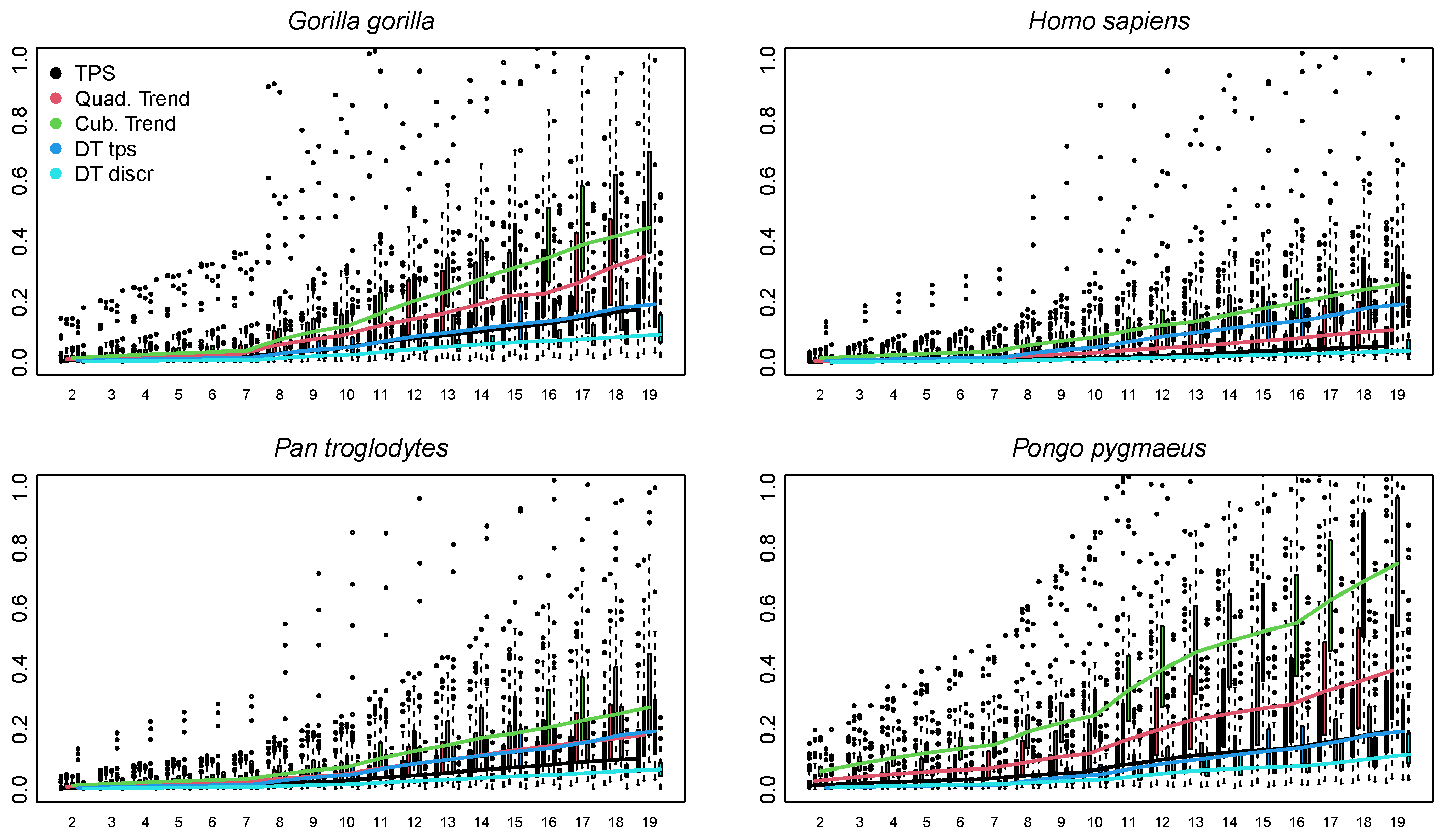
As mentioned in Section 4 we provide the $d_R$ distance between U computed using the discrete way on triangles and tetrahedra and the distances between those obtained by TPS, QT, and CT interpolants for the four Hominidae species, separately taking the youngest prediction as source. Figure 20 shows results for the tetrahedralization structure; the three methods do not differ considerably, with TPS always being below QT and CT, especially for Pongo pygmaeus, and with differences among methods that are augmented at the oldest ages.

Figure 21 shows results obtained using the triangulation structure; the pattern is similar to that observed for tetrahedra, but TPS is much more evidently below the other two methods. Again, differences increase with the form differences between the source and the target.

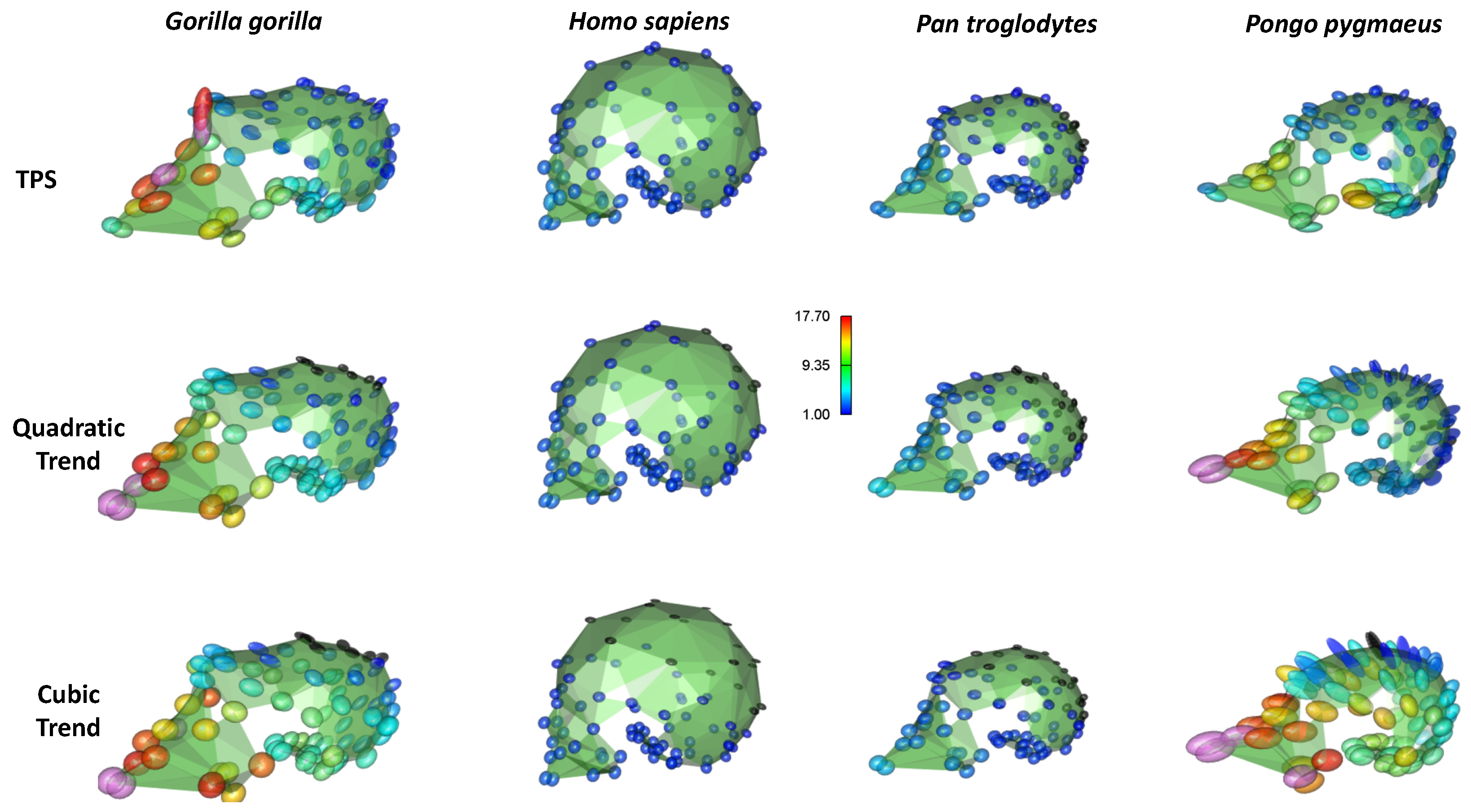
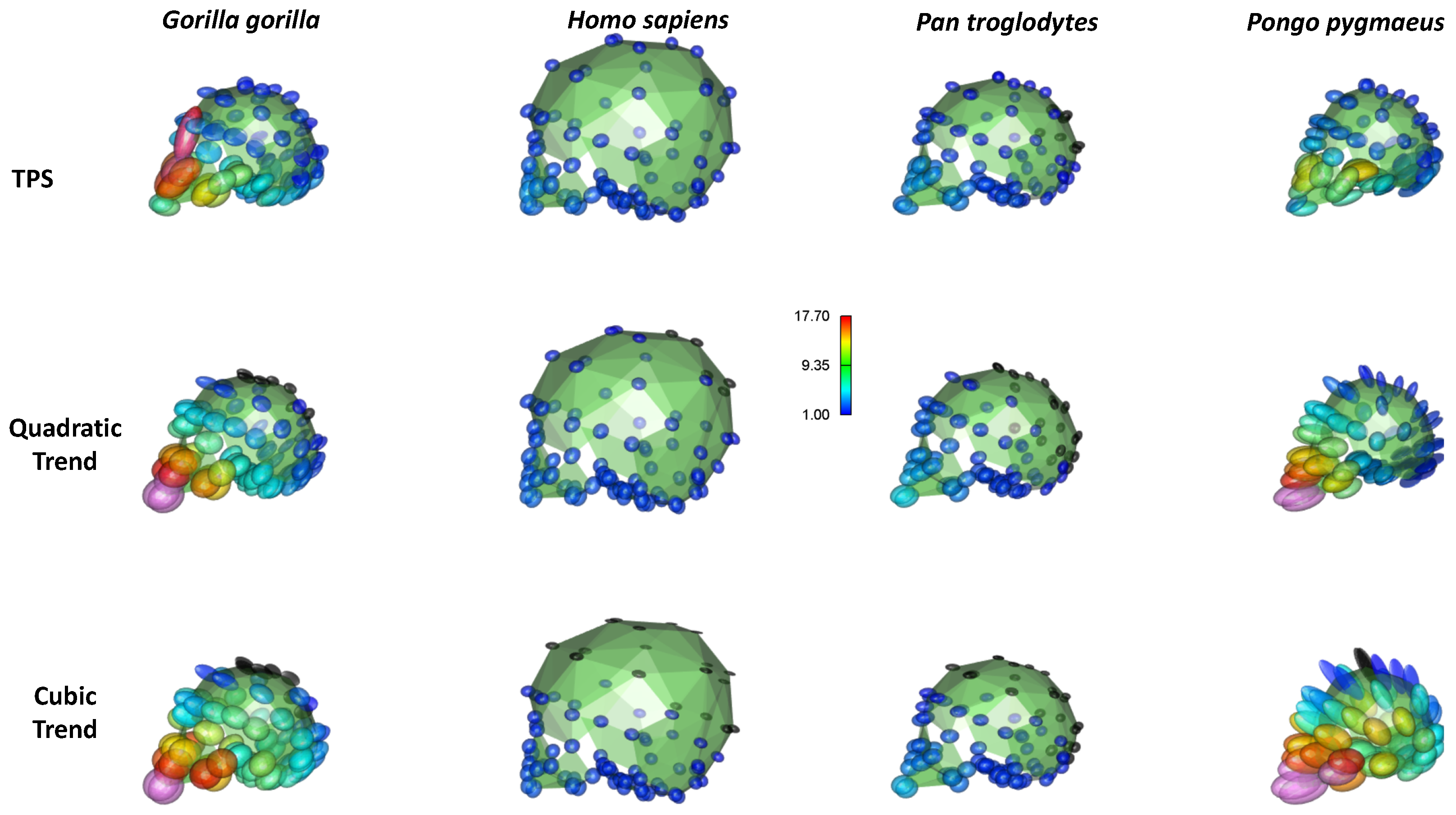
We note, in both Figure 20 and Figure 21, that per-species tensors evaluated via TPS behave consistently when compared to tensors computed via TPS on transported data. We consider an expected result to be the very small distance shown by tensors computed on transported data using the discrete method. We present in Figure 22 and Figure 23 the U and F tensors computed using TPS, QT, and CT for the youngest-to-oldest predictions across the four species. The color gradient legend is proportional to det(U), indicating m-Volume changes. We show the two figures in slightly different perspectives to augment the reader’s appreciation of the growth process. Tensor ellipsoids highlight significant differences in cranial growth among the primate species examined. The following considerations focus on the patterns revealed by TPS tensors, while differences among methods will be discussed afterward.

In Gorilla gorilla, cranial growth is characterized by a vertical expansion of the central region of the supraorbital torus, a posterior–lateral shift of the orbital floor, and an anterior projection of the nasal region in adult stages. The zygomatic process moves antero-medially, while the palatal region expands posteriorly. The neurocranium undergoes antero-posterior growth, accompanied by the development of midsagittal and lambdoidal cranial crests. The central portion of the basioccipital extends anteriorly, while its lateral parts shift antero-medially along the cranial base [66].

In Homo sapiens, the nasal region expands vertically during cranial growth, leading to slight dental prognathism due to the anterior expansion of the palatal region. The neurocranium grows in both the antero-posterior and medio-lateral directions [67,68].

Pan troglodytes exhibits a pattern of facial prognathism during growth, involving the nasal, zygomatic, and upper oral regions. The neurocranium expands primarily in the medio-lateral direction, while the cranial base extends both antero-posteriorly and medio-laterally around the foramen magnum [69].

In Pongo pygmaeus, facial growth occurs predominantly in the antero-posterior direction, leading to dental prognathism and a concave morphology between the nasal and upper oral regions. The upper neurocranium expands medio-laterally, while the squamous part of the occipital bone undergoes both vertical and lateral expansion. Additionally, the basioccipital region of the cranial base show anteriorly directed growth [70].

Given the significant limitations of a two-dimensional projection of a single snapshot, we strongly encourage readers to run the provided R scripts (included in the Supplementary Material) to generate the 3D versions of these figures. This will allow for a more comprehensive appreciation of the anatomical details and provide the ability to interact with fully movable and zoomable 3D models.

As for the comparison between TPS, QT, and CT, it is striking at first glance that QT and CT extracts tensors that appear, in some anatomical districts, exaggeratedly flat, as in the cranial vault of Homo sapiens and Pan troglodytes or exaggeratedly enlarged, such as in the mouth of Pongo pygmaeus. These deformations do not match some notions regarding skull growth in these species: for example, in Homo sapiens, it is well known that the neurocranium grows more “spherically” with respect to extant Hominidae [23]; this signal is not captured by the quasi-flat tensors imputed by QT and CT but emerges from TPS tensors on Homo sapiens vault.

6. Discussion

6.1. Effectiveness of PCA on Tensor Components and Dependence on Interpolants

The results presented above suggest that PCA on tensor components, evaluated at homologous landmark positions, can effectively capture global deformative signals by using unique tensor components as local features, much like displacement components in traditional GPA followed by PCA. However, this approach fundamentally depends on the choice of the interpolant used to evaluate tensors. In our examples, we leveraged the properties of TPS, QT, and CT interpolation functions. Among them, TPS proved particularly versatile, efficiently recovering pre-assigned tensors in a highly challenging 2D simulated experiment; least squares methods, in particular CT, can work well for small deformations but for the large ones fail in recovering assigned tensors.

The primary objective of this study was to explore the feasibility of using individual tensor components in ordination analyses in group-wise structured data as an alternative to PT methods, thereby avoiding the choice for a Riemannian connection and metric. Nevertheless, the selection of an appropriate interpolant remains essential. We did not explore the Riemannian structure of the manifold generated by the “tensor’s space” (see below). We cannot eliminate a certain quota of arbitrariness here due to the choice of the interpolant (if tensors are evaluated using the interpolant’s first derivative) or to that of a triangulation/tetrahedralization structure (when tensors are estimated in the discrete way).

As stated in the Section 4, we did not employ specific non-linear PCA approaches here, as we believe doing so would have hindered a direct comparison with standard morphometric methods.

6.2. U or F

At the conclusion of the analyses presented here, one might ask the following question: What is the most rational choice between using U or F tensors? To answer this, we must be more specific about the fundamental nature of these two types of tensors. As stated in the Section 1 and Section 4, $\mathbf{U}=\sqrt{\mathbf{C}}=\sqrt{{\mathbf{F}}^T\mathbf{F}}$; this operation removes the local infinitesimal rotations encoded in each $\mathbf{F}$, making $\mathbf{U}$ symmetric (ideally, positive definite). In other words, removing a global mean rotation, such as the one found in GPA, OPA, Resistant Fit, or modified ordinary Procrustes analysis (MOPA, see [13]) eliminates the same rotation from all $\mathbf{F}$ tensors in a target before their estimation; different targets have, of course, different mean global rotations with respect to the source. $\mathbf{U}$ tensors are not affected by global rotation, making the choice of alignment entirely inconsequential. However, if tensors are not estimated from actual individuals (as in a deformation series) but instead derived from some kind of mean (i.e., GPA mean), then the alignment criterion used for mean estimation becomes an important consideration; however, the complete set of $\mathbf{U}$ tensors estimated within a deformation encodes the reciprocal rotations between each $\mathbf{U}$. This ensures that, given a compatible field of $\mathbf{U}$, the deformed state can be fully reconstructed using $\mathbf{U}$ only, as demonstrated in the 2D bending simulations. The $\mathbf{F}$ tensors emerge as a formal necessity from the displacement field resulting from integrating the $\mathbf{U}$ tensors into the compatible geometric domain of the undeformed state. If a continuous (integrable) interpolant is used, compatibility is formally ensured when mapping $\mathbf{U}$ back onto the undeformed state. However, this is not the case if a different template is used, such as in a PT framework [17]; in order to verify that a field of $\mathbf{U}$ is still compatible with a given geometric domain, i.e., a function $\psi$ exists so that $\nabla {\left(\psi \right)}^T\nabla \left(\psi \right)=\mathbf{C}$, the Riemannian curvature calculated using the field of $\mathbf{C}$ as a metric tensor must be 0 [71]. If this condition is met, then $\mathbf{C}$ is a fully Euclidean metric and there exists a configuration in the Euclidean space that has $\mathbf{C}$ as a local metric. In conclusion, the use of $\mathbf{U}$ is fully justified and remains independent of the choice of global alignment criterion.

6.3. Comparison with PT Methods and Performance on Real 3D Data

Using a real 3D dataset of ontogenetic trajectories from four hominoid species, we assessed the effectiveness of this approach by comparing (via correlations between Euclidean distances computed on PC scores blocks) its performance with a highly effective PT method, i.e., DT. The results indicate that this approach is viable and produces meaningful patterns. The reciprocal relationships among species’ ontogenetic trajectories remain virtually identical when comparing the PCA space of transported data with the PCA space obtained from U recovered via TPS (with slightly lower consistency when using F). While QT and CT also perform reasonably well, their correlations are lower. This difference is further reflected in the youngest–oldest predictions across the four species: in certain regions of the skull, such as the cranial vault, QT and CT tensors (visualized as ellipsoids) appear nearly flat, suggesting local deformation patterns that do not align with established knowledge of hominoid skull growth. We consider particularly relevant the comparison of the $d_R$ distance (derived from finite-element-based tensors on per-species trajectories) between tensors estimated on per-species trajectories via TPS and those estimated on data transported according to DT. As expected, tensors estimated on DT-transported shapes using the discrete approach adhere very closely to the original finite-element-based tensors. In contrast, tensors estimated via TPS align much more closely with those estimated directly on per-species trajectories. While this outcome might also be anticipated, we regard it as non-trivial, since it corroborates both the DT procedure and per-species evaluation as coherent strategies for appropriate data centering when analyzing deformational trajectories.

6.4. Benchmarking Interpolants

It could be argued that, in biological studies, no absolute null model exists, making it difficult to favor one interpolant over another. For this reason, we first conducted a benchmark experiment to assess how different interpolants recover pre-assigned, known tensors. In this evaluation, TPS demonstrated greater versatility than QT and CT, likely because TPS better preserves localness compared to the least squares method, an essential property when studying infinitesimal local deformation. In fact, TPS has zero error in predictions, unlike other approaches (such as least squares). The least squares method, as a CT, can still be used for small deformations. Smoothing splines introduce an error term in the data predicted during a spatial interpolation, but this was not explored here.

6.5. Relevance to Other Fields and Broader Implications

In other fields, principal strains derived from tensors have been used to infer significant local differences between groups. For instance, in the study of cardiac mechanics, tensors and principal strain estimation have become standard tools for analyzing mechanical behavior across a wide range of diseases ([72,73], and references therein, [74]). These measures are routinely subjected to statistical analyses in a manner quite similar to that employed by [42], among others.

7. Caveats, Limitations, and Future Directions

We consider it essential to outline some aspects that should be carefully considered when applying the procedure described in this study. These points serve both as guidelines to enhance user awareness and as a foundation for making fully informed methodological choices. Some are intended as prompts for further exploration of tensor properties rather than as obstacles.

7.1. Scaling in (a) Shape Space (SS)

This study does not explore the properties of tensors when evaluated in deformations estimated between shapes scaled in SS (or at a specific unit size measure). As stated in Section 1, within the GM paradigm, scaling to unit CS results in a curved manifold, making it a non-linear operation. When shapes undergo scaling at unit CS, centering, and alignment to the mean according to GPA, they are mapped onto a hyper-hemisphere of radius 1. To facilitate the safe application of standard multivariate methods, coordinates are typically projected (either orthogonally or, less commonly, stereographically) onto a tangent plane at the mean shape. The fully spherical Kendall’s Shape Space, on the other hand, is obtained by scaling all shapes by $1/cos\left(\rho \right)$, where $\rho$ represents the angular Procrustes distance between a given shape and the consensus (see [75,76] for further details). In cases with “small” variations, the projection procedure ensures no significant biases. Strain tensors consider m-Volume as a measure of local “size” change. One could propose to scale all forms at unit m-Volume (only a constrained and dense Delaunay triangulation or tetrahedralization allows a precise evaluation of it). Since scaling to unit m-Volume defines a hyper-hyperbolic manifold [13], an appropriate projection procedure would be necessary to fully integrate tensor-based methods into a rigorous “tensor SS” framework. A first step could involve scaling coordinates by the $m^{th}$ root of the m-Volume, or by $det\left(A\right)$’s $m^{th}$ root, where A is the $m\times m$ matrix representing the linear component of the deformation (which can be estimated in different ways or simply at unitary m-Volume; see [77]; [13] Section 4.1). Future research should investigate how different scaling choices impact tensor-based analyses and whether a standardized projection method can be established for robust statistical applications. While one might argue that scaling affects tensors in the same manner as coordinates, since they are merely divided by a scalar, this holds only for identical shapes ($\rho =0$). In a sample of different shapes, reciprocal scaling strongly influences the relative positions in ordination space (see Figure 2 of the present paper).

7.2. Impact of Landmark Distribution

The accuracy and robustness of tensor estimations depend heavily on landmark density and distribution, as interpolation is performed exclusively on the homologous landmarks; the tensor’s evaluation points could be everywhere. A too sparse, or a too spatially unbalanced, landmark configuration may fail to adequately capture local deformations, leading to oversimplified or misleading tensor estimates. But this aspect affects GPA alignment too, of course. Moreover, a landmark configuration distributed solely on outlines or surfaces, while passively enabling the estimation of the interpolation map, does not adequately inform the interpolant about the conditions within the interior. If one aims to estimate tensors in the interior, one must be aware that, although the interpolant provides information about deformation, this information emerges from a sort of “black box” because no landmarks were provided in this region of space. Optimizing landmark distribution is therefore crucial for obtaining reliable tensor representations, and this depends on data quality, the capabilities of the capture system, the digitization process, and, ultimately, the biological hypothesis underlying the study. As for the number of landmarks we note that recently some debates have been raised (see [78,79]) albeit mainly referred to tests for morphological integration.

7.3. Choice of Interpolants

There is no universally optimal interpolant. While TPS has demonstrated high versatility in capturing local deformations, QT and CT offer advantages in terms of the simplicity of their coefficients (see [39] for other properties) and have been demonstrated to be valuable for small deformations. However, QT assumes that the second derivative is constant, implying that the variation of the first gradient is uniform in all spatial directions, an assumption that is difficult to conceive as consistent with real data. One could argue that a model is chosen not to perfectly match reality but rather to generate explanatory (ideally causal, though this is not always possible) hypotheses. However, a model should always be assessed based on its ability to achieve the objectives set by the research program. If the goal is to evaluate local deformations and use them in hypothesis-testing statistics, its ability to capture locality is a crucial aspect to consider. The selection of an interpolant should then be context-dependent, balancing local accuracy and global regularization based on the specific application. In this study, we did not test B-splines, smoothing splines, or quadratic TPS, a variant of TPS that minimizes the sum of squared third derivative across the entire space [39,80]; in this case, for $m=2$, the kernel function is $h^{4}log\left(h\right)$, instead of $h^{2}log\left(h\right)$; for $m=3$, it is $h^3$, instead of $-\left|h\right|$ with h the pairwise Euclidean distance.

The results presented in Figure 9, Figure 10 and Figure 11 suggest that for small deformations, a least squares approach can still provide valuable results, but the choice of the interpolant remains an a priori choice that the researcher should evaluate case-by-case. The deep knowledge of the theoretical simulation or of the real biological problem under investigation must always guide the final decision.

7.4. Suitability for Longitudinal Deformations

We advocate that tensor-based approaches are particularly effective in analyzing longitudinal deformations in SSS. This includes ontogenetic and allometric studies or the temporal mechanical deformation of a single structure (e.g., a beating heart), where deformation trajectories over time can be systematically compared. In this context, tensor-based methods could be considered an alternative to PT, avoiding the need to explicitly define a Riemannian connection and a metric.

7.5. Tensors vs. Displacements

Tensors are not intended as a replacement for displacements. This study does not claim that tensors are inherently superior to displacement-based methods. Displacements, though subject to the arbitrariness of the alignment choice (see [40] for a recent evaluation of the Resistant Fit alignment) and scaling strategies, remain the only objective datum we have and are the direct input for tensor estimation using any kind of interpolant. Tensors, however, provide a complementary perspective, capturing additional information about local deformation patterns that might be lost in traditional landmark-based analyses. The choice between tensors and displacements ultimately depends on the research question and the scale of deformation being investigated. For example, in those situations where meaningful anatomical directions are defined, such as in cardiac mechanics with longitudinal, circumferential, and radial directions, the projections of the tensor’s $v$ along these directions allow effective hypothesis-testing statistics.

7.6. Integration of Recovered Tensors for Shape Prediction

A crucial methodological improvement that remains to be implemented is the integration of recovered tensors (or those predicted by PCA axes) over the spatial domain of a reference template to visualize corresponding predicted shapes. However, convergence/compatibility issues and computational complexity pose significant challenges that must be addressed to make this approach fully operational.

References

1. Dryden, I.L.; Mardia, K.V. Statistical Shape Analysis, with Applications in R, 2nd ed.; Wiley: Chichester, UK, 2016. [Google Scholar]
2. Bookstein, F. A Course in Morphometrics for Biologists: Geometry and Statistics for Studies of Organismal Form; Cambridge University Press: Cambridge, UK, 2018. [Google Scholar] [CrossRef] [Scilit]
3. Bookstein, F. Landmark Methods for Forms Without Landmarks: Morphometrics of Group Differences in Outline Shape. Med. Image Anal. 1997, 1, 225–243. [Google Scholar] [CrossRef] [Scilit]
4. Baylac, M.; Frieß, M. Fourier descriptors, Procrustes superimposition, and data dimensionality: An example of cranial shape analysis in modern human populations. In Modern Morphometrics in Physical Anthropology; Slice, D., Ed.; University of Chicago: Chicago, IL, USA, 2005; pp. 145–165. [Google Scholar] [CrossRef] [Scilit]
5. Guigui, N.; Pennec, X. Parallel transport, a central tool in geometric statistics for computational anatomy: Application to cardiac motion modeling. In Handbook of Statistics 46; Nielsen, F., Rao, A., Rao, C., Eds.; Elsevier: Oxford, UK, 2022; pp. 285–326. [Google Scholar] [CrossRef] [Scilit]
6. Goswami, A.; Polly, P. Methods for studying morphological integration and modularity. In Quantitative Methods in Paleobiology; Alroy, J., Hunt, E., Eds.; Paleontological Society Special Publications, Ithaca: New York, NY, USA, 2010; pp. 213–243. [Google Scholar] [CrossRef] [Scilit]
7. Varano, V.; Gabriele, S.; Teresi, L.; Dryden, I.L.; Puddu, P.E.; Torromeo, C.; Piras, P. The TPS direct transport: A new method for transporting deformations in the size-and-shape space. Int. J. Comput. Vis. 2017, 124, 384–408. [Google Scholar] [CrossRef] [Scilit]
8. Piras, P.; Guigui, N.; Varano, V. Comparison of different parallel transport methods for the study of deformations in 3D cardiac data. J. Math. Imaging Vis. 2024, 66, 393–415. [Google Scholar] [CrossRef] [Scilit]
9. Guigui, N.; Maignant, E.; Trouvé, A.; Pennec, X. Parallel transport on Kendall shape spaces. In Geometric Science of Information; Lecture Notes in Computer Science; Springer: Cham, Switzerland, 2021; Volume 12829, pp. 103–110. [Google Scholar] [CrossRef] [Scilit]
10. Piras, P.; Evangelista, A.; Gabriele, S.; Nardinocchi, P.; Teresi, L.; Torromeo, C.; Schiariti, M.; Varano, V.; Puddu, P.E. 4D-analysis of left ventricular heart cycle using Procrustes motion analysis. PLoS ONE 2014, 9, 86–96. [Google Scholar] [CrossRef] [Scilit]
11. Piras, P.; Teresi, L.; Traversetti, L.; Varano, V.; Gabriele, S.; Kotsakis, T.; Raia, P.; Puddu, P.E. The conceptual framework of ontogenetic trajectories: Parallel transport allows the recognition and visualization of pure deformation patterns. Evol. Dev. 2016, 18, 182–200. [Google Scholar] [CrossRef] [Scilit] [PubMed]
12. Piras, P.; Torromeo, C.; Evangelista, A.; Esposito, G.; Nardinocchi, P.; Teresi, L.; Madeo, A.; Re, F.; Chialastri, C.; Schiariti, M.; et al. Non-invasive prediction of genotype positive-phenotype negative in hypertrophic cardiomyopathy by 3D modern shape analysis. Exp. Physiol. 2019, 104, 1688–1700. [Google Scholar] [CrossRef] [Scilit]
13. Varano, V.; Piras, P.; Gabriele, S.; Teresi, L.; Nardinocchi, L.; Dryden, I.; Torromeo, C.; Puddu, P. The decomposition of deformation: New metrics to enhance shape analysis in medical imaging. Med. Im. Anal. 2018, 46, 35–56. [Google Scholar] [CrossRef] [Scilit]
14. Huckemann, S.; Hotz, T.; Munk, A. Intrinsic MANOVA for Riemannian Manifolds with an Application to Kendall’s Space of Planar Shapes. IEEE Trans. Pattern Anal. Mach. Intell. 2010, 32, 593–603. [Google Scholar] [CrossRef] [Scilit]
15. Bernardino, G.; Dargent, T.; Camara, O.; Duchateau, N. Stranger Things: Discrete Differential Geometry for Transporting Right Ventricular Deformation Across Meshes. In Proceedings of the 12th International Conference on Functional Imaging and Modeling of the Heart, Lyon, France, 19–22 June 2023; pp. 338–346. [Google Scholar] [CrossRef] [Scilit]
16. Teresi, L.; Milicchio, F.; Gabriele, S.; Piras, P. Shape deformation from metric’s transport. Int. J. Non-Linear Mech. 2020, 119, 103326. [Google Scholar] [CrossRef] [Scilit]
17. Milicchio, F.; Varano, V.; Gabriele, S.; Teresi, L.; Puddu, P.E.; Piras, P. Parallel transport of local strains. Comput. Methods Biomech. Biomed. Eng. Imaging Vis. 2019, 7, 520–528. [Google Scholar] [CrossRef] [Scilit]
18. Sumner, R.W.; Popović, J. Deformation transfer for triangle meshes. ACM Trans. Graph. 2004, 23, 399–405. [Google Scholar] [CrossRef] [Scilit]
19. Sumner, R.W.; Popović, J. Deformation Transfer for Triangle Meshes. In Seminal Graphics Papers: Pushing the Boundaries, Volume 2, 1st ed.; Association for Computing Machinery: New York, NY, USA, 2023. [Google Scholar] [CrossRef] [Scilit]
20. Piras, P.; Varano, V.; Louis, M.; Profico, A.; Durrleman, S.; Charlier, B.; Milicchio, F.; Teresi, L. Transporting deformations of face emotions in the shape spaces: A comparison of different approaches. J. Math. Imaging Vis. 2021, 63, 875–893. [Google Scholar] [CrossRef] [Scilit]
21. Mitteroecker, P.; Schaefer, K. Thirty years of geometric morphometrics: Achievements, challenges, and the ongoing quest for biological meaningfulness. Yearb. Biol. Anth. 2022, 178, 181–210. [Google Scholar] [CrossRef] [Scilit]
22. McNulty, K.; Frost, S.; Strait, D. Examining affinities of the Taung child by developmental simulation. J. Hum. Evol. 2006, 51, 274–296. [Google Scholar] [CrossRef] [Scilit]
23. Neubauer, S.; Hublin, J.J.; Gunz, P. The evolution of modern human brain shape. Sci. Adv. 2018, 4, eaao5961. [Google Scholar] [CrossRef] [Scilit]
24. Hotz, I.; Sreevalsan-Nair, J.; Hagen, H.; Hamann, B. Tensor field reconstruction based on eigenvector and eigenvalue interpolation. In Scientific Visualization: Advanced Concepts. Dagstuhl Follow-Ups; Dagstuhl-Leibniz-Zentrum für Informatik: Wadern, Germany, 2010; Volume 1, pp. 110–123. [Google Scholar] [CrossRef] [Scilit]
25. Bookstein, F. Morphometric Tools for Landmark Data: Geometry and Biology; Cambridge University Press: Cambridge, UK, 1991. [Google Scholar] [CrossRef] [Scilit]
26. Bookstein, F. Transformations of Quadrilaterals, Tensor Fields, and Morphogenesis. In Mathematical Essays on Growth and the Emergence of Form; Antonelli, P., Ed.; University of Alberta Press: Edmonton, AB, Canada, 1985; pp. 221–265. Available online: https://www.worldcat.org/title/mathematical-essays-on-growth-and-the-emergence-of-form/oclc/13524845 (accessed on 15 December 2025).
27. Bookstein, F. Tensor Biometrics for Changes in Cranial Shape. Ann. Hum. Biol. 1984, 11, 413–437. [Google Scholar] [CrossRef] [Scilit]
28. Bookstein, F.L. Describing a craniofacial anomaly: Finite elements and the biometrics of landmark locations. Am. J. Phys. Anthropol. 1987, 74, 495–509. [Google Scholar] [CrossRef] [Scilit]
29. Gurtin, M.E. An Introduction to Continuum Mechanics; Academic Press: New York, NY, USA, 1981. [Google Scholar]
30. Klingenberg, C. How exactly did the nose get that long? A critical rethinking of the Pinocchio effect and how shape changes relate to landmarks. Evol. Biol. 2021, 48, 115–127. [Google Scholar] [CrossRef] [Scilit]
31. Truesdell, C.A. Cauchy and the modern mechanics of continua. Rev. Hist. Sci. 1992, 45, 5–24. [Google Scholar] [CrossRef] [Scilit]
32. Spencer, A.J.M. George Green and the foundations of the theory of elasticity. J. Eng. Math. 2015, 95, 5–6. [Google Scholar] [CrossRef] [Scilit]
33. Bookstein, F. The Measurement of Biological Shape and Shape Change; Lecture Notes in Biomath; Springer: London, UK; Berlin, Germany, 1978; Volume 24. [Google Scholar] [CrossRef] [Scilit]
34. Bookstein, F. The Geometry of Craniofacial Growth Invariants. Am. J. Orthod. 1983, 83, 221–234. [Google Scholar] [CrossRef] [Scilit] [PubMed]
35. Bookstein, F. A Geometric Foundation for the Study of Left Ventricular Motion: Some Tensor Considerations. In Digital Cardiac Imaging; Buda, A., Delp, E., Eds.; Martinus Nijhoff Publishers: Leiden, The Netherlands, 1985; pp. 65–83. [Google Scholar]
36. Bookstein, F.; Green, W. A Feature Space for Edgels in Images with Landmarks. J. Math. Imaging Vis. 1993, 3, 231–261. [Google Scholar] [CrossRef] [Scilit]
37. O’Higgins, P. Studies of craniofacial growth and development: A review. Proc. Australas. Soc. Hum. Biol. 1992, 5, 329–343. [Google Scholar]
38. O’Higgins, P.; Dryden, I. Sexual dimorphism in hominoids: Further studies of craniofacial shape differences in Pan, Gorilla and Pongo. J. Hum. Evol. 1993, 24, 183–205. [Google Scholar] [CrossRef] [Scilit]
39. Bookstein, F. Quadratic Trends: A Morphometric Tool Both Old and New. Evol. Biol. 2024, 51, 1–44. [Google Scholar] [CrossRef] [Scilit]
40. Marugán-Lobón, J. Métodos resistentes basados en la mediana en el marco actual de la Morfometría Geométrica contemporánea. Sp. J. Pal. 2025, 40, 125–132. [Google Scholar] [CrossRef] [Scilit]
41. Bookstein, F. Reworking Geometric Morphometrics into a Methodology of Transformation Grids. Evol. Biol. 2023, 50, 275–299. [Google Scholar] [CrossRef] [Scilit]
42. Márquez, E.; Cabeen, R.; Woods, R.; Houle, D. The measurement of local variation in shape. Evol. Biol. 2012, 39, 419–439. [Google Scholar] [CrossRef] [Scilit] [PubMed]
43. Richtsmeier, J.T. Craniofacial growth in Apert syndrome as measured by finite element scaling analysis. Acta Anat. 1988, 133, 50–56. [Google Scholar] [CrossRef] [Scilit]
44. Pennec, X. Statistical computing on manifolds: From Riemannian geometry to computational anatomy. In Emerging Trends in Visual Computing. ETVC 2008; Lecture Notes in Computer Science; Nielsen, F., Ed.; Springer: London, UK; Berlin, Germany, 2009; Volume 5416, pp. 347–386. [Google Scholar] [CrossRef] [Scilit]
45. Ashburner, J.; Ridgway, G. Tensor-based morphometry. In Brain Mapping: An Encyclopedic Reference; Toga, A., Ed.; Academic Press: Oxford, UK, 2015; pp. 383–394. [Google Scholar] [CrossRef] [Scilit]
46. Ashburner, J.; Friston, K. Voxel-based morphometry-the methods. NeuroImage 2000, 11, 805–821. [Google Scholar] [CrossRef] [Scilit] [PubMed]
47. Ashburner, J.; Friston, K. Why voxel-based morphometry should be used. NeuroImage 2001, 14, 1238–1243. [Google Scholar] [CrossRef] [Scilit]
48. Bookstein, F. Voxel-Based Morphometry Should Not Be Used with Imperfectly Registered Images. NeuroImage 2001, 14, 1454–1462. [Google Scholar] [CrossRef] [Scilit] [PubMed]
49. Whitcher, B.; Wisco, J.; Hadjikhani, N.; Tuch, D. Statistical group comparison of diffusion tensors via multivariate hypothesis testing. Magn. Res. Med. 2007, 57, 1065–1074. [Google Scholar] [CrossRef] [Scilit] [PubMed]
50. Wickham, H.; Hester, J.; Chang, W.; Bryan, J. devtools: Tools to Make Developing R Packages Easier, R package version 2.4.5; RStudio: Boston, MA, USA, 2022.
51. Piras, P.; Profico, A.; Pandolfi, L.; Raia, P.; Di Vincenzo, F.; Mondanaro, A.; Castiglione, S.; Varano, V. Current options for visualization of local deformation in modern shape analysis applied to paleobiological case studies. Front. Earth Sci. 2020, 8, 66. [Google Scholar] [CrossRef] [Scilit]
52. Colorado-Cervantes, I.; Varano, V.; Teresi, L. Stress-free morphing by means of compatible distortions. Phys. Rev. E 2022, 106, 015003. [Google Scholar] [CrossRef] [Scilit]
53. Schölkopf, B.; Smola, A.; Müller, K.R. Nonlinear Component Analysis as a Kernel Eigenvalue Problem. Neural Comput. 1998, 10, 1299–1319. [Google Scholar] [CrossRef] [Scilit]
54. Huckemann, S.; Hotz, T.; Munk, A. Intrinsic Shape Analysis: Geodesic PCA for Riemannian Manifolds Modulo Isometric Lie Group Actions. Stat. Sin. 2010, 20, 1–58. [Google Scholar]
55. Dryden, I.L.; Koloydenko, A.; Zhou, D. Non-Euclidean statistics for covariance matrices, with applications to diffusion tensor imaging. Ann. Appl. Stat. 2009, 3, 1102–1123. [Google Scholar] [CrossRef] [Scilit]
56. Mitteröcker, P.; Bookstein, F. The Ontogenetic Trajectory of the Phenotypic Covariance Matrix, with Examples from Craniofacial Shape in Rats and Humans. Evolution 2009, 63, 727–737. [Google Scholar] [CrossRef] [Scilit]
57. Arsigny, V.; Fillard, P.; Pennec, X.; Ayache, N. Log-Euclidean metrics for fast and simple calculus on diffusion tensors. Magn. Reson. Med. 2006, 56, 411–421. [Google Scholar] [CrossRef] [Scilit]
58. Profico, A.; Piras, P.; Buzi, C.; Di Vincenzo, F.; Lattarini, F.; Melchionna, M.; Veneziano, A.; Raia, P.; Manzi, G. The evolution of cranial base and face in Cercopithecoidea and Hominoidea: Modularity and morphological integration. Am. J. Primatol. 2017, 79, e22721. [Google Scholar] [CrossRef] [Scilit] [PubMed]
59. Dean, M.; Wood, B. Developing Pongid Dentition and Its Use for Ageing Individual Crania in Comparative Cross-Sectional Growth Studies. Folia Primatol. 1981, 36, 111–127. [Google Scholar] [CrossRef] [Scilit]
60. Smith, B.H.; Crummett, T.L.; Brandt, K.L. Ages of eruption of primate teeth: A compendium for aging individuals and comparing life histories. Yearb. Phys. Anthropol. 1994, 37, 177–231. [Google Scholar] [CrossRef] [Scilit]
61. Dirks, W.; Bowman, J. Life history theory and dental development in four species of catarrhine primates. J. Hum. Evol. 2007, 53, 309–320. [Google Scholar] [CrossRef] [Scilit]
62. Lieberman, D.; Carlo, J.; Ponce de León, M.; Zollikofer, C. A geometric morphometric analysis of heterochrony in the cranium of chimpanzees and bonobos. J. Hum. Evol. 2007, 52, 647–662. [Google Scholar] [CrossRef] [Scilit]
63. Lafarge, T.; Pateiro-Lopez, B. alphashape3d: Implementation of the 3D Alpha-Shape for the Reconstruction of 3D Sets from a Point Cloud, R package version 1.3.2; RStudio: Boston, MA, USA, 2023.
64. Bookstein, F.L. Random walk as a null model for high-dimensional morphometrics of fossil series: Geometrical considerations. Paleobiology 2013, 39, 52–74. [Google Scholar] [CrossRef] [Scilit]
65. Mitteroecker, P.; Gunz, P.; Bookstein, F. Heterochrony and geometric morphometrics: A comparison of cranial growth in Pan paniscus versus Pan troglodytes. Evol. Dev. 2005, 7, 244–258. [Google Scholar] [CrossRef] [Scilit]
66. Berge, C.; Penin, X. Ontogenetic allometry, heterochrony, and interspecific differences in the skull of African apes, using tridimensional Procrustes analysis. Am. J. Phys. Anthropol. 2004, 124, 124–138. [Google Scholar] [CrossRef] [Scilit]
67. Lieberman, D.E.; McBratney, B.M.; Krovitz, G. The evolution and development of cranial form in Homo sapiens. Proc. Natl. Acad. Sci. USA 2002, 99, 1134–1139. [Google Scholar] [CrossRef] [Scilit] [PubMed]
68. Martinez-Maza, C.; Rosas, A.; Nieto-Díaz, M. Postnatal changes in the growth dynamics of the human face revealed from bone modelling patterns. J. Anat. 2013, 223, 228–241. [Google Scholar] [CrossRef] [Scilit] [PubMed]
69. Bastir, M.; Rosas, A. Facial heights: Evolutionary relevance of postnatal ontogeny for facial orientation and skull morphology in humans and chimpanzees. J. Hum. Evol. 2004, 47, 359–381. [Google Scholar] [CrossRef] [Scilit]
70. Hens, S.M. Ontogeny of craniofacial sexual dimorphism in the orangutan (Pongo pygmaeus). I: Face and palate. Am. J. Primatol. 2005, 65, 149–166. [Google Scholar] [CrossRef] [Scilit]
71. Minozzi, M.; Nardinocchi, P.; Teresi, L.; Varano, V. Growth-induced compatible strains. Math. Mech. Sol. 2017, 22, 62–71. [Google Scholar] [CrossRef] [Scilit]
72. Lee, Y.; Cansız, B.; Sveric, K.; Linke, A.; Kaliske, M. Assessment of LV structural remodelling by the application of the finite element method to 3D echocardiography data. Comput. Methods Biomech. Biomed. Eng. Imaging Vis. 2024, 12, 2314592. [Google Scholar] [CrossRef] [Scilit]
73. Piras, P.; Colorado-Cervantes, I.; Nardinocchi, P.; Gabriele, S.; Varano, V.; Esposito, G.; Teresi, L.; Torromeo, C.; Puddu, P.E. Geometry Does Impact on the Plane Strain Directions of the Human Left Ventricle, Irrespective of Disease. J. Cardiovasc. Dev. Dis. 2022, 9, 393. [Google Scholar] [CrossRef] [Scilit]
74. Topriceanu, C.C.; Al-Farih, M.; Joy, G.; Chan, F.; Webber, M.; Ilie-Ablachim, D.C.; Shiwani, H.; Tamang, M.; Banks, C.; Pettit, S.; et al. The Cardiovascular Magnetic Resonance Phenotype of Lamin Heart Disease. JACC Cardiovasc. Imaging 2025, 18, 644–660. [Google Scholar] [CrossRef] [Scilit]
75. Rohlf, F.J. Shape statistics: Procrustes superimpositions and tangent spaces. J. Class. 1999, 16, 197–223. [Google Scholar] [CrossRef] [Scilit]
76. Slice, D.E. Landmark coordinates aligned by Procrustes analysis do not lie in Kendall’s shape space. Syst. Biol. 2001, 50, 141–149. [Google Scholar] [CrossRef] [PubMed]
77. Rohlf, F.J.; Bookstein, F.L. Computing the uniform component of shape variation. Syst. Biol. 2003, 52, 66–69. [Google Scholar] [CrossRef]
78. Cardini, A. Less tautology, more biology? A comment on “high-density” morphometrics. Zoomorphology 2020, 139, 513–529. [Google Scholar] [CrossRef] [Scilit]
79. Goswami, A.; Watanabe, A.; Felice, R.; Bardua, C.; Fabre, A.; Polly, P. High-density morphometric analysis of shape and integration: The good, the bad, and the not-really-a-problem. Integr. Comp. Biol. 2019, 59, 669–683. [Google Scholar] [CrossRef] [Scilit] [PubMed]
80. Bookstein, F. After Landmarks. In Modern Morphometrics in Physical Anthropology; Slice, D., Ed.; Springer: London, UK; Berlin, Germany, 2005; pp. 49–71. [Google Scholar] [CrossRef] [Scilit]
Figure 1. Summary box of possible options offered by strain tensor computation related to shape analysis.
Mathematics 14 00012 g001
Figure 2. Panels 1–3 from the left: Bending of a parallelepiped of length L and height H. H = L/ π : the reference parallelepiped bends by π radians at R = L/ π and becomes a closed cylinder at R = L/(2 π ). Panels 4–6 from the left: H = 2L/ π : the reference parallelepiped bends by π /2 radians at R = 2L/ π and becomes a half cylinder at R = L/ π , with the minimum radius avoiding self-penetration. All six configurations are stress-free. Modified from ([52]).
Mathematics 14 00012 g002
Figure 3. Two-dimensional forms (centered, not aligned) of the three bending series described in the present paper. Top row = “Pure bending”; middle row = “Isotropic bending”; bottom row = “Nematic bending”. Given the parametrization singular when R = , the starting forms are not perfectly regular. This does not affect results or their interpretation in any way. Curvature angle R values: 200 / π , 20 / π , 10 / π , 4 / π , 2 / π , 1 / π , 0.8 / π , 0.5 / π .
Mathematics 14 00012 g003
Figure 4. Size variation of the bending datasets with size defined as m-Volume or CS. Black = “Pure bending”; red = “Isotropic bending”; green = “Nematic bending”.
Mathematics 14 00012 g004
Figure 5. An adult male Pan troglodytes mesh showing the 81 landmarks digitized on the original acquired surface, as well as the triangulation structure derived from the digitized landmarks only. We also show, in the bottom right panel, the tetrahedralization structure (expanded to show single elements) decided using the “alphashape3d” R package (see text).
Mathematics 14 00012 g005
Figure 6. d R distance between assigned benchmark tensors and tensors recovered according to TPS, QT and CT. Top row: all 7 deformed states. Bottom row: details of the first 4 states. Lines connect median values of the distributions.
Mathematics 14 00012 g006
Figure 7. PCA performed on displacement and on tensors (F and U) recovered via TPS. In these scatterplots, as well as in the following ones, the symbol ‘+’ should be interpreted as ‘followed by’.
Mathematics 14 00012 g007
Figure 8. PCA performed on tensors (F and U) recovered via QT and CT.
Mathematics 14 00012 g008
Figure 9. Predictions of QT and CT for the pure bending data with the first form as source and all the others as targets (aligned via OPA on the source). TPS predictions coincide with target shapes. Landmarks color refers to the d R distance for TPS (first row) CT and QT; violet denotes values exceeding the upper limit of the range. The two color legends correspond to the first three deformed states (on the left) and to the last four (on the right). The deformation grid has been set as a triangular grid coincident with the body domain in order to properly show the presence or absence of folding within the body.
Mathematics 14 00012 g009
Figure 10. Predictions of QT and CT for the isotropic bending data with the first form as source and all the others as targets (aligned via OPA on the source). TPS predictions coincide with target shapes. Landmark color refers to the d R distance for TPS (first row), CT and QT; violet denotes values exceeding the upper limit of the range. The two color legends correspond to the first three deformed states (on the left) and to the last four (on the right). The deformation grid has been set as a triangular grid coincident with the body domain in order to properly show the presence or absence of folding within the body.
Mathematics 14 00012 g010
Figure 11. Predictions of QT and CT for the nematic bending data with the first form as source and all the others as targets (aligned via OPA on the source). TPS predictions coincide with target shapes. Landmark color refers to the d R distance for TPS (first row), CT and QT; violet denotes values exceeding the upper limit of the range. The two color legends correspond to the first three deformed states (on the left) and to the last four (on the right). The deformation grid has been set as a triangular grid coincident with the body domain in order to properly show the presence or absence of folding within the body.
Mathematics 14 00012 g011
Figure 12. Benchmark v plotted on source according to deformed states together with those recovered by the three interpolants for the pure (normal) bending case. v was additionally scaled according to a proper common scalar, 0.03, fo the sake of visualization. The color legends indicate the λ value (1 means no deformation). In the central row of forms, the benchmark λ 1 / λ 2 = 1 for this case.
Mathematics 14 00012 g012
Figure 13. The same as in Figure 12 but for the isotropic bending case. The benchmark λ 1 / λ 2 = 1 everywhere.
Mathematics 14 00012 g013
Figure 14. The same as in Figure 12 but for the nematic bending case. In this case, the benchmark λ 1 / λ 2 = k , with k constant everywhere for each deformative step and increasingly larger toward the last step.
Mathematics 14 00012 g014
Figure 15. Vertical red lines indicate the expected value of the λ 1 / λ 2 ratio for the isotropic and nematic bending according to the benchmark assigned tensor; they are plotted on the density distributions of the actual λ 1 / λ 2 computed on recovered tensors.
Mathematics 14 00012 g015
Figure 16. Preliminary results on primate skull data. Top-left panel: GPA in SSS followed by PCA on observed data. The top-right and bottom-right panels show the relationships between age and predicted values and PC1 of GPA, followed by PCA on predicted forms, respectively. The bottom-left panel shows the PC1-PC2 scatterplot of GPA followed by PCA in SSS performed on forms predicted at homologous ages. The point dimension is proportional to age.
Mathematics 14 00012 g016
Figure 17. PCA results coming from the different approaches described in the text. The point dimension is proportional to age. All analyses performed done in SSS. Colours as in Figure 16.
Mathematics 14 00012 g017
Figure 18. Correlation between Euclidean distances among PC scores coming from PCA performed on DT data and correlations from PCAs performed on tensors components upon TPS, QT and CT. The value of the correlation coefficient is indicated.
Mathematics 14 00012 g018
Figure 19. Correlation between Euclidean distances among PC scores coming from PCA performed on data coming from GPA in SSS and those from PCAs performed on tensor components upon TPS using GPA mean as reference. The value of the correlation coefficient is indicated.
Mathematics 14 00012 g019
Figure 20. d R distance between U computed using the discrete method on tetrahedra and those obtained by TPS, QT, and CT, taking the youngest prediction as source. We also add the d R distance from tensors computed on per-species trajectories and those computed on data transported according to DT.
Mathematics 14 00012 g020
Figure 21. d R distance between U computed using the discrete method on triangles and those obtained by TPS, QT, and CT, taking the youngest prediction as source. We also add the d R distance from tensors computed on per-species trajectories and those computed on data transported according to DT.
Mathematics 14 00012 g021
Figure 22. U tensors computed between forms predicted at the youngest ages as a source and the oldest ages as a target. U tensors are plotted on the per-species source, i.e., the forms predicted at the youngest ages. Tensors are represented as ellipsoids resulting from deforming a sphere of unitary radius and successively scaled by a common scalar quantity, 4, for the sake of visualization. Colors refer to tensors’ determinants, which informs of the local m-Volume expansion (>1) or contraction (<1); as we deal with forms growing in SSS, thus without eliminating size, we set “1” as the minimum value in the color scale gradient legend. Violet indicates values beyond the scale’s maximum, and black indicates values below the scale’s minimum, thus suggesting a local contraction.
Mathematics 14 00012 g022
Figure 23. As in Figure 22 but using F tensors plotted on targets, i.e., per-species predictions at the oldest ages.
Mathematics 14 00012 g023