Random Generalized Additive Logistic Forest: A Novel Ensemble Method for Robust Binary Classification

Abstract

Ensemble methods have proven highly effective in enhancing predictive performance by combining multiple models. We introduce a novel ensemble approach, the Random Generalized Additive Logistic Forest (RGALF), which integrates generalized additive models (GAMs) within a random forest framework to improve binary classification tasks. Unlike traditional random forests, which rely on piecewise constant predictions in terminal nodes, RGALF fits GAM logistic regression (LR) models to the data in each terminal node, enabling it to capture complex nonlinear relationships and interactions among predictors. By aggregating these node-specific GAMs, RGALF addresses multicollinearity, enhances interpretability, and achieves superior bias–variance tradeoffs, particularly in nonlinear settings. Theoretical analysis confirms that RGALF achieves Stone’s optimal rates for additive models ($\mathcal{O}(n^{-2k/(2k+d)}$) under appropriate conditions, outperforming the slower convergence of traditional random forests ($\mathcal{O}\left(n^{-2/3}\right)$). Furthermore, empirical results demonstrate RGALF’s effectiveness across both simulated and real-world datasets. In simulations, RGALF demonstrates superior performance over random forests (RFs), reducing variance by up to 69% and bias by 19% in nonlinear settings, with significant MSE improvements (0.032 vs. RF’s 0.054 at $n=1000$), while achieving optimal convergence rates ($\mathcal{O}\left(n^{-0.48}\right)$ vs. RF’s $\mathcal{O}\left(n^{-0.29}\right)$). On real-world medical datasets, RGALF attains near-perfect accuracy and AUC: 100% accuracy/AUC for Heart Failure and Hepatitis C (HCV) prediction, 99% accuracy/100% AUC for Pima Diabetes, and 98.8% accuracy/100% AUC for Indian Liver Patient (ILPD), outperforming state-of-the-art methods. Notably, RGALF captures complex biomarker interactions (BMI–insulin in diabetes) missed by traditional models.

1. Introduction

Random forests (RFs) have revolutionized machine learning by combining the robustness of the ensemble with the capacity to handle high-dimensional data [1]. Despite their success, a critical limitation persists in classification tasks: terminal nodes rely on simplistic averaging of class probabilities, assuming linear separability and failing to capture complex nonlinear decision boundaries [2]. This shortcoming is exacerbated in real-world datasets, where class probabilities exhibit intricate dependencies on predictors, such as medical diagnostics with high-curvature risk surfaces or financial data with nonlinear feature interactions. While logistic regression (LR) offers interpretability, its linearity constraint similarly limits performance in these settings [3].

Recent hybrid approaches attempt to bridge this gap, but retain fundamental limitations. Penalized Logistic Tree Regression (PLTR) integrates LR with tree splits to model credit risk, achieving 87% accuracy, but preserves linear terminal nodes [4]. Spline-based probability calibration embeds splines as post hoc adjustments in RF for medical diagnostics, improving cancer classification accuracy by 5% [5], yet treats splines as external calibrators rather than intrinsic model components. GAMBoost combines Gradient Boosting with additive models for groundwater prediction (83% accuracy) but sacrifices ensemble diversity by using a sequential training framework [6]. Structural refinements like genetic algorithm-optimized RF [7] and kernelized splits [8] focus on split criteria or kernel transformations, leaving terminal node linearity unaddressed. Even variants focusing on interpretability, such as the transparent rule generator RF [9] or oblique forests [10], simplify node structures without explicit nonlinear modeling capacity. These efforts underscore a persistent gap: no framework replaces RF’s averaging mechanism with flexible, interpretable nonlinear models capable of capturing complex probability surfaces.

The resurgence of generalized additive models (GAMs) offers a promising path forward. GAMs model nonlinear relationships through additive spline terms, achieving 79.9% accuracy in ICU mortality prediction [11] and outperforming linear models in high-curvature settings. However, prior integrations with machine learning either treat GAMs as standalone classifiers [11] or combine them with deep learning at the cost of interpretability [12]. Meanwhile, domain-specific applications highlight unmet demands: healthcare models like hybrid ensemble deep learning for stroke detection (94% sensitivity [13]) and finance frameworks such as XGBoost-LR hybrids for credit risk (88.79% precision [14]) achieve strong performance but lack structured interpretability for non-linear effects. This disconnect between accuracy, interpretability, and flexibility motivates our work.

We propose the Random Generalized Additive Logistic Forest (RGALF), which replaces RF’s terminal node averaging with node-specific GAMs. This integration enables two fundamental advances:

• Nonlinear Probability Estimation: By modeling class probabilities through smooth spline terms, RGALF captures high-curvature decision boundaries and nonlinear feature interactions that elude traditional RF and LR.
• Structured Interpretability: Each terminal GAM provides additive interpretations of feature contributions, preserving the benefits of the RF ensemble while offering insights into non-linear effects, a critical advantage in fields such as healthcare and finance.

RGALF addresses three unmet needs: (1) modeling nonlinear class probabilities without sacrificing interpretability, (2) maintaining ensemble robustness through bootstrap aggregation, and (3) scaling computationally to high-dimensional datasets. Unlike prior hybrids that retrofit linear models or post hoc splines, RGALF embeds GAMs directly into RF’s architecture, enabling end-to-end learning of additive nonlinear effects.

This paper is organized as follows: Section 2 formalizes the RGALF framework and outlines its algorithmic innovations. Section 3 presents the simulation study. Section 4 discusses the results, which validate the performance of RGALF against benchmark models on both synthetic and real-world datasets, including applications in the medical field. Section 5 addresses the implications and limitations of the study, while Section 6 concludes the paper and suggests directions for future research.

2. Random Generalized Additive Logistic Forest (RGALF)

2.1. Preliminaries: Random Forest Framework

Let $\mathcal{D}={\left\{({\mathbf{x}}_i,y_i)\right\}}_{i=1}^n$ where ${\mathbf{x}}_i\in \mathcal{X}\subseteq {\mathbb{R}}^p$ and $y_i\in \{0,1\}$. A random forest constructs B decision trees ${\left\{T_b\right\}}_{b=1}^B$, each trained on a bootstrap sample ${\mathcal{D}}_b$. At each node, the optimal split $(j^{*},s^{*})$ is chosen from a randomly selected subset of features $\mathcal{M}\subseteq \{1,\dots ,p\}$ with $\left|\mathcal{M}\right|=m$ (where $m\ll p$ is a hyperparameter) by solving

$$(j^{*},s^{*})=arg\underset{(j,s)\in \mathcal{M}\times {\mathcal{T}}_j}{max}\Delta I(j,s),$$

where ${\mathcal{T}}_j$ denotes the set of candidate thresholds for feature j, and the Gini impurity reduction $\Delta I(j,s)$ is

$$\Delta I(j,s)=I\left(\mathcal{P}\right)-{\displaystyle \frac{N_L}{N}}I\left(\mathcal{L}\right)-{\displaystyle \frac{N_R}{N}}I\left(\mathcal{R}\right),$$

with parent node $\mathcal{P}$, left/right children $\mathcal{L},\mathcal{R}$, and Gini impurity, as follows:

$$I\left(\mathcal{A}\right)=1-\sum _{{\displaystyle k=0}}^1{\left({\displaystyle \frac{1}{\left|\mathcal{A}\right|}}\sum _{i\in \mathcal{A}}\mathbb{I}(y_i=k)\right)}^2.$$

Let ${\mathcal{L}}_b\left(\mathbf{x}\right)$ denote the terminal leaf node in tree $T_b$ containing $\mathbf{x}$. The classical random forest (RF) estimates class probabilities via naive averaging within leaves, as follows:

$${\widehat{p}}_b\left(\mathbf{x}\right)={\displaystyle \frac{1}{|{\mathcal{L}}_b\left(\mathbf{x}\right)|}}\sum _{i\in {\mathcal{L}}_b\left(\mathbf{x}\right)}{y}_i.$$

The ensemble aggregates these as ${\widehat{p}}_{\mathrm{RF}}\left(\mathbf{x}\right)={\displaystyle \frac{1}{B}}{\sum }_{b=1}^B{\widehat{p}}_b\left(\mathbf{x}\right)$. While effective in low-curvature regimes, this local averaging incurs bias when the true conditional probability $p\left(\mathbf{x}\right)=\mathbb{E}[y\mid \mathbf{x}]$ exhibits rapid spatial variation.

Theorem 1 

(Local Homogeneity Limitation). For twice differentiable $p\left(\mathbf{x}\right)$, the RF bias satisfies

$$|\mathbb{E}\left[{\widehat{p}}_{\mathrm{RF}}\left(\mathbf{x}\right)\right]-p\left(\mathbf{x}\right)|\le C·\mathrm{diam}{\left(\mathcal{L}\left(\mathbf{x}\right)\right)}^2,$$

where $C={\displaystyle \frac{1}{2}}{sup}_{\mathbf{x}}{\parallel \mathcal{H}\left(\mathbf{x}\right)\parallel }_F$ is a constant depending on the maximum Frobenius norm of the Hessian $\mathcal{H}\left(\mathbf{x}\right)$, and $\mathit{diam}\left(\mathcal{L}\left(\mathbf{x}\right)\right)={sup}_{{\mathbf{x}}^{\prime },{\mathbf{x}}^{″}\in \mathcal{L}\left(\mathbf{x}\right)}{\parallel {\mathbf{x}}^{\prime }-{\mathbf{x}}^{″}\parallel }_2$ is the leaf diameter.

Proof. 

Let ${\overline{\mathbf{x}}}_{\mathcal{L}}={\displaystyle \frac{1}{\left|\mathcal{L}\right(\mathbf{x}\left)\right|}}{\sum }_{{\mathbf{x}}^{\prime }\in \mathcal{L}\left(\mathbf{x}\right)}{\mathbf{x}}^{\prime }$ be the leaf centroid. A second-order Taylor expansion of $p\left({\mathbf{x}}^{\prime }\right)$ about ${\overline{\mathbf{x}}}_{\mathcal{L}}$ gives

$$p\left({\mathbf{x}}^{\prime }\right)=p\left({\overline{\mathbf{x}}}_{\mathcal{L}}\right)+\nabla p{\left({\overline{\mathbf{x}}}_{\mathcal{L}}\right)}^{\top }({\mathbf{x}}^{\prime }-{\overline{\mathbf{x}}}_{\mathcal{L}})+{\displaystyle \frac{1}{2}}{({\mathbf{x}}^{\prime }-{\overline{\mathbf{x}}}_{\mathcal{L}})}^{\top }\mathcal{H}\left({\overline{\mathbf{x}}}_{\mathcal{L}}\right)({\mathbf{x}}^{\prime }-{\overline{\mathbf{x}}}_{\mathcal{L}})+R\left({\mathbf{x}}^{\prime }\right),$$

where the remainder $R\left({\mathbf{x}}^{\prime }\right)$ satisfies $|R\left({\mathbf{x}}^{\prime }\right)|\le {\displaystyle \frac{M}{6}}{\parallel {\mathbf{x}}^{\prime }-{\overline{\mathbf{x}}}_{\mathcal{L}}\parallel }_2^3$ for $M={sup}_{\mathbf{x}}{\parallel {\nabla }^{3}p\left(\mathbf{x}\right)\parallel }_2$. Averaging over $\mathcal{L}\left(\mathbf{x}\right)$,

$$\mathbb{E}\left[{\widehat{p}}_{\mathrm{RF}}\left(\mathbf{x}\right)\right]-p\left(\mathbf{x}\right)=\underset{\mathrm{Quadratic}\mathrm{Term}}{\underbrace{{\displaystyle \frac{1}{2}}\mathrm{tr}\left(\mathcal{H}\left(\mathbf{x}\right){\pm }_{\mathcal{L}}\right)}}+\underset{\mathrm{Residual}}{\underbrace{{\displaystyle \frac{1}{\left|\mathcal{L}\right|}}{\displaystyle \sum _{{\mathbf{x}}^{\prime }\in \mathcal{L}}}R\left({\mathbf{x}}^{\prime }\right)}}.$$

Bounding the residual:

$$\left|{\displaystyle \frac{1}{\left|\mathcal{L}\right|}}\sum R\left({\mathbf{x}}^{\prime }\right)\right|\le {\displaystyle \frac{M}{6}}·\mathrm{diam}{\left(\mathcal{L}\right)}^3.$$

Since $\mathrm{diam}{\left(\mathcal{L}\right)}^3=o\left(\mathrm{diam}{\left(\mathcal{L}\right)}^2\right)$ as $\mathrm{diam}\left(\mathcal{L}\right)\to 0$, the residual is absorbed into the constant C, yielding

$$|\mathbb{E}\left[{\widehat{p}}_{\mathrm{RF}}\left(\mathbf{x}\right)\right]-p\left(\mathbf{x}\right)|\le {\displaystyle \frac{1}{2}}{\parallel \mathcal{H}\left(\mathbf{x}\right)\parallel }_F{\parallel {\pm }_{\mathcal{L}}\parallel }_F+{\displaystyle \frac{M}{6}}\mathrm{diam}{\left(\mathcal{L}\right)}^3\le C·\mathrm{diam}{\left(\mathcal{L}\right)}^2,$$

with $C={\displaystyle \frac{1}{2}}{sup}_{\mathbf{x}}{\parallel \mathcal{H}\left(\mathbf{x}\right)\parallel }_F+{\displaystyle \frac{M}{6}}{sup}_{\mathbf{x}}\mathrm{diam}\left(\mathcal{L}\left(\mathbf{x}\right)\right)$. □

Remark 1. 

The bias term exposes the following two failure modes:

1.

High Curvature:  When ${\parallel \mathcal{H}\left(\mathbf{x}\right)\parallel }_F$ is large (e.g., near steep logistic slopes), even small leaves incur quadratic bias.

2.

Axis-Aligned Partitioning:  Axis-aligned splits produce leaves with ${\pm }_{\mathcal{L}}$ having large eigenvalues along certain features, amplifying bias in high dimensions.

2.2. RGALF Terminal Node Generalized Additive Logistic Model

The RGALF replaces RF’s terminal node averaging with localized GAM. For terminal node ${\mathcal{L}}_b\left(\mathbf{x}\right)$ (containing $n_b$ samples) and splitting features ${\mathcal{S}}_b\subseteq \{1,\dots ,p\}$, RGALF models

$$\mathrm{logit}\left(p_b\left(\mathbf{x}\right)\right)={\beta }_{b0}+\sum _{j\in {\mathcal{S}}_b}{f}_{bj}\left(x_j\right),$$

where $f_{bj}\left(x_j\right)={\sum }_{k=1}^K{\gamma }_{bjk}{\varphi }_k\left(x_j\right)$ uses B-spline basis functions ${\left\{{\varphi }_k\right\}}_{k=1}^K$ of order d (e.g., cubic splines: $d=4$). Knots ${\left\{{\xi }_{jk}\right\}}_{k=1}^{K-d}$ for feature j are placed uniformly over $[a_j,b_j]$, as follows:

$${\xi }_{jk}=a_j+{\displaystyle \frac{k}{K-d+1}}(b_j-a_j).$$

The roughness penalty matrix ${\mathbf{S}}_j\in {\mathbb{R}}^{K\times K}$ for feature j has entries, as follows:

$${\left({\mathbf{S}}_j\right)}_{kl}={\int }_{a_j}^{b_j}{\varphi }_k^{″}\left(x_j\right){\varphi }_l^{″}\left(x_j\right)d{x}_j.$$

2.3. Parameter Estimation via Penalized Likelihood

The penalized log-likelihood for node ${\mathcal{L}}_b$ is

$${\ell }_b\left({\mathit{\theta }}_b\right)=\sum _{i\in {\mathcal{L}}_b}\left[y_i{\eta }_{bi}-log(1+e^{{\eta }_{bi}})\right]-{\displaystyle \frac{1}{2}}{\gamma }_b^{\top }\left({\lambda }_b\mathbf{S}\right){\gamma }_b,$$

where ${\gamma }_b={({\gamma }_{bj1},\dots ,{\gamma }_{bjK})}_{j\in {\mathcal{S}}_b}$, $\mathbf{S}=\mathrm{blkdiag}{\left({\mathbf{S}}_j\right)}_{j\in {\mathcal{S}}_b}$, and ${\lambda }_b$ controls smoothness. The estimation of ${\mathit{\theta }}_b$ is performed via the Iteratively Reweighted Least Squares (IRLS) Algorithm. At iteration t,

• Compute probabilities ${\widehat{p}}_{bi}^{\left(t\right)}={\mathrm{logit}}^{-1}\left({\eta }_{bi}^{\left(t\right)}\right)$;
• Weights $w_i^{\left(t\right)}={\widehat{p}}_{bi}^{\left(t\right)}(1-{\widehat{p}}_{bi}^{\left(t\right)})$ form diagonal matrix ${\mathbf{W}}_b^{\left(t\right)}$;
• Working responses: $z_i^{\left(t\right)}={\eta }_{bi}^{\left(t\right)}+{\displaystyle \frac{y_i-{\widehat{p}}_{bi}^{\left(t\right)}}{w_i^{\left(t\right)}}}$;
• Solve penalized weighted least squares, as follows:

  $$\left({\mathbf{X}}_b^{\top }{\mathbf{W}}_b^{\left(t\right)}{\mathbf{X}}_b+{\lambda }_b\mathbf{S}\right){\mathit{\theta }}_b^{(t+1)}={\mathbf{X}}_b^{\top }{\mathbf{W}}_b^{\left(t\right)}{\mathbf{z}}_b^{\left(t\right)},$$

  where ${\mathbf{X}}_b$ contains spline basis evaluations for features ${\mathcal{S}}_b$.

Consequently, the smoothing parameter ${\lambda }_b$ is optimized via the restricted maximum likelihood (REML), as follows:

$${\ell }_{\mathrm{REML}}\left({\lambda }_b\right)={\displaystyle \frac{1}{2}}log|{\mathbf{X}}_b^{\top }{\mathbf{W}}_b{\mathbf{X}}_b+{\lambda }_b\mathbf{S}|-{\displaystyle \frac{1}{2}}log{\left|{\lambda }_b\mathbf{S}\right|}_{+}-{\displaystyle \frac{1}{2}}{({\mathbf{z}}_b-{\mathbf{X}}_b{\widehat{\mathit{\theta }}}_b)}^{\top }{\mathbf{W}}_b({\mathbf{z}}_b-{\mathbf{X}}_b{\widehat{\mathit{\theta }}}_b),$$

where ${|·|}_{+}$ denotes the product of non-zero eigenvalues.

Notation

• $B_k\left(x_j\right)$: B-spline basis function of order 3;
• ${\gamma }_{jk}$: Spline coefficients with ridge penalty $\lambda$;
• $n_{\min }$: Minimum node size for GAM fitting (default = 10);
• ${\mathrm{logit}}^{-1}$: Inverse logistic function ${(1+e^{-\eta })}^{-1}$.

2.4. Ensemble Aggregation and Variance Reduction

The RGALF ensemble predictor

$${\widehat{p}}_{\mathrm{RGALF}}\left(\mathbf{x}\right)={\displaystyle \frac{1}{B}}{\displaystyle \sum _{b=1}^B}{p}_b\left(\mathbf{x}\right),$$

achieves variance reduction through the following:

Theorem 2 

(Bias Reduction). Let the true conditional probability $p\left(\mathbf{x}\right)=\mathbb{E}\left[y\right|\mathbf{x}]$ belong to the additive class, as follows:

$$p\left(\mathbf{x}\right)=g^{-1}\left({\beta }_0+{\displaystyle \sum _{j=1}^p}{f}_j\left(x_j\right)\right),$$

where g is the logit link function and $f_j\in {\mathcal{H}}_k$, a Hölder space of order $k\ge 2$. Under RGALF with B-spline bases of order $d\ge k-1$, for any $\mathbf{x}\in \mathcal{X}$,

$$|\mathbb{E}\left[{\widehat{p}}_{\mathrm{RGALF}}\left(\mathbf{x}\right)\right]-p\left(\mathbf{x}\right)|\le C_1{h}^{2k}+C_2{B}^{-1},$$

where $h={max}_b\mathrm{diam}\left({\mathcal{L}}_b\left(\mathbf{x}\right)\right)$. Comparatively, RF satisfies

$$|\mathbb{E}\left[{\widehat{p}}_{\mathrm{RF}}\left(\mathbf{x}\right)\right]-p\left(\mathbf{x}\right)|\le C_3{h}^2+C_4{B}^{-1}.$$

Proof. 

• Let ${\widehat{p}}_b\left(\mathbf{x}\right)$ be the GAM estimate in tree b. Decompose

  $$\mathbb{E}[{\widehat{p}}_b\left(\mathbf{x}\right)-p\left(\mathbf{x}\right)]=\underset{\mathrm{Estimation}\mathrm{error}}{\underbrace{\mathbb{E}[{\widehat{p}}_b\left(\mathbf{x}\right)-p_b^{*}\left(\mathbf{x}\right)]}}+\underset{\mathrm{Approximation}\mathrm{error}}{\underbrace{p_b^{*}\left(\mathbf{x}\right)-p\left(\mathbf{x}\right)}},$$

  where $p_b^{*}$ is the best approximation in the GAM space.
• By de Boor’s theorem [15], for $f_j\in {\mathcal{H}}_k$ and B-splines of order d,

  $$\parallel f_j-{\widehat{f}}_{bj}{\parallel }_{\infty }\le C{h}^k\mathrm{where}h=\underset{j}{max}\mathrm{diam}\left({\mathcal{L}}_b\left({\mathbf{x}}_j\right)\right).$$

  This gives $|p_b^{*}\left(\mathbf{x}\right)-p\left(\mathbf{x}\right)|\le C^{\prime }{h}^{2k}$.
• Since trees are identically distributed,

  $$\mathbb{E}[{\widehat{p}}_{\mathrm{RGALF}}-p\left(\mathbf{x}\right)]={\displaystyle \frac{1}{B}}{\displaystyle \sum _{b=1}^B}\mathbb{E}[{\widehat{p}}_b-p]\le C_1{h}^{2k}+\mathcal{O}\left(B^{-1}\right).$$

  □

Remark 2. 

The bias of the model is influenced by the smoothness of the basis functions, such as in the case of cubic splines (when $k=2$). This improved rate is due to the fact that the nonlinear terms in the GAM can capture curvature, which reduces the need for local averaging. As a result, $p\left(\mathbf{x}\right)$ can exhibit sharp transitions or interactions, situations in which traditional random forests (RFs) typically face challenges.

Theorem 3 

(Variance Reduction). Let ${\sigma }^2\left(\mathbf{x}\right)=\mathrm{Var}\left(y\right|\mathbf{x})$. Under the same conditions as Theorem 2,

$$\mathrm{Var}\left({\widehat{p}}_{\mathrm{RGALF}}\left(\mathbf{x}\right)\right)\le \mathrm{Var}\left({\widehat{p}}_{\mathrm{RF}}\left(\mathbf{x}\right)\right)-{\displaystyle \frac{\Delta \left(\mathbf{x}\right)}{B}},$$

where $\Delta \left(\mathbf{x}\right)={\sum }_{b=1}^B\left[\mathbb{E}\left(p_b^2\right)-\mathbb{E}{\left(p_b\right)}^2\right]\ge 0$.

Proof. 

For an ensemble of B trees,

$$\mathrm{Var}\left({\widehat{p}}_{\mathrm{RGALF}}\right)={\displaystyle \frac{1}{B^2}}{\displaystyle \sum _{b=1}^B}\mathrm{Var}\left(p_b\right)+{\displaystyle \frac{2}{B^2}}\sum _{b<b^{\prime }}\mathrm{Cov}(p_b,p_{b^{\prime }}).$$

RGALF’s localized GAMs reduce individual tree variances, as follows:

$$\mathrm{Var}\left(p_b^{\mathrm{RGALF}}\right)\le \mathrm{Var}\left(p_b^{\mathrm{RF}}\right)-\mathbb{E}\left[{(p_b-\mathbb{E}{p}_b)}^2\right],$$

since GAMs’ smoothness constraints suppress high-frequency noise.

Let $\Delta \left(\mathbf{x}\right)={\sum }_{b=1}^B\left[\mathrm{Var}\left(p_b^{\mathrm{RF}}\right)-\mathrm{Var}\left(p_b^{\mathrm{RGALF}}\right)\right]\ge 0$, as variances are non-negative. Then, RF trees exhibit positive covariance due to shared splits, as follows:

$${\mathrm{Cov}}_{\mathrm{RF}}(p_b,p_{b^{\prime }})=\mathbb{E}\left[(p_b-\mathbb{E}{p}_b)(p_{b^{\prime }}-\mathbb{E}{p}_{b^{\prime }})\right]\ge 0.$$

This implies that the RGALF’s node-specific GAMs decorrelate trees by introducing heterogeneity, as follows:

$${\mathrm{Cov}}_{\mathrm{RGALF}}(p_b,p_{b^{\prime }})={\mathrm{Cov}}_{\mathrm{RF}}(p_b,p_{b^{\prime }})-\eta \left(\mathbf{x}\right),$$

where $\eta \left(\mathbf{x}\right)=\mathbb{E}\left[(f_b\left(\mathbf{x}\right)-\mathbb{E}{f}_b\left(\mathbf{x}\right))(f_{b^{\prime }}\left(\mathbf{x}\right)-\mathbb{E}{f}_{b^{\prime }}\left(\mathbf{x}\right))\right]\ge 0$, as GAMs’ nonlinear terms $f_b,f_{b^{\prime }}$ reduce dependence on shared splits.

Substituting into the variance expression,

$$\mathrm{Var}\left({\widehat{p}}_{\mathrm{RGALF}}\right)=\mathrm{Var}\left({\widehat{p}}_{\mathrm{RF}}\right)-\underset{\ge 0}{\underbrace{{\displaystyle \frac{\Delta \left(\mathbf{x}\right)}{B}}}}-\underset{\ge 0}{\underbrace{{\displaystyle \frac{2}{B^2}}{\displaystyle \sum _{b<b^{\prime }}}\eta \left(\mathbf{x}\right)}}\le \mathrm{Var}\left({\widehat{p}}_{\mathrm{RF}}\right).$$

Both subtracted terms are non-negative by construction. □

Theorem 4 

(L² Consistency). Assume the following:

1.

Regularity: $\mathbb{E}\left[y^2\right]<\infty$, $p\left(\mathbf{x}\right)$ Lipschitz continuous.

2.

Complexity: Spline bases satisfy $K=\mathcal{O}\left(n^{\alpha }\right)$, $0<\alpha <1$.

3.

Growth conditions: $B\to \infty$, $h_n\to 0$, $n{h}_n^{2k}\to \infty$.

Then

$$\underset{n,B\to \infty }{lim}\mathbb{E}\left[{({\widehat{p}}_{\mathrm{RGALF}}\left(\mathbf{x}\right)-p\left(\mathbf{x}\right))}^2\right]=0a.s.$$

Proof. 

Let

$$\mathbb{E}\left[{(\widehat{p}-p)}^2\right]=\underset{{\mathrm{Bias}}^2}{\underbrace{{(\mathbb{E}\left[\widehat{p}\right]-p)}^2}}+\underset{\mathrm{Variance}}{\underbrace{\mathrm{Var}\left(\widehat{p}\right)}}.$$

From Theorem 2, ${\mathrm{Bias}}^2\le C_1^2{h}^{4k}$. With $h_n\to 0$, ${\mathrm{Bias}}^2\to 0$.

Theorem 3 gives $\mathrm{Var}\left(\widehat{p}\right)\le \mathcal{O}\left(B^{-1}\right)+\mathcal{O}\left(n^{-1}{h}_n^{-d}\right)$. Under growth conditions,

$$\underset{n,B\to \infty }{lim}\mathrm{Var}\left(\widehat{p}\right)=0.$$

Applying the Borel–Cantelli lemma [16] with ${\sum }_{n=1}^{\infty }\mathbb{P}\left(\right|\widehat{p}-p|>ϵ)<\infty$, ensured by exponential inequalities for U-statistics. □

Remark 3 

(Discussion of Regularity Conditions). The theoretical guarantees of RGALF rely on three fundamental regularity conditions that balance model flexibility with statistical consistency. We elaborate on each condition below, including their mathematical implications and practical consequences.

• Lipschitz Continuity: For the true conditional probability function $p\left(\mathbf{x}\right)=\mathbb{E}\left[y\right|\mathbf{x}]$, we require

  $$\exists L>0s.t.|p\left(\mathbf{x}\right)-p\left({\mathbf{x}}^{\prime }\right)|\le L{\mathbf{x}-{\mathbf{x}}^{\prime }}_2\forall \mathbf{x},{\mathbf{x}}^{\prime }\in \mathcal{X}$$

  -

  Ensure that the spline basis coefficients $\left\{{\gamma }_{bjk}\right\}$ remain bounded, controlling approximation error in terminal node GAMs. For B-splines of the order d, this guarantees

  $${f_{bj}-f_{bj}^{*}}_{L_2}\le C{h}_b^{d+1}$$

  where $h_b$ is the node diameter and $f_{bj}^{*}$ is the optimal spline approximation.

  -

  The practical implication justifies using low-order splines (cubic/d = 4) instead of higher-order polynomials. Violations (e.g., discontinuous $p\left(\mathbf{x}\right)$) require adaptive knot placement.

  -

  Testable Condition: Estimated via empirical Lipschitz constant, as follows:

  $$\widehat{L}=\underset{{\mathbf{x}}_i\ne {\mathbf{x}}_j}{max}{\displaystyle \frac{|\widehat{p}\left({\mathbf{x}}_i\right)-\widehat{p}\left({\mathbf{x}}_j\right)|}{{{\mathbf{x}}_i-{\mathbf{x}}_j}_2}}$$

• Basis Growth Rate: The spline basis dimension K must satisfy

  $$K=\mathcal{O}\left(n^{\alpha }\right),0<\alpha <{\displaystyle \frac{2k}{2k+d}}$$

  where k is the Hölder smoothness order of $p\left(\mathbf{x}\right)$, and d is the feature dimension.

  -

  Bias–Variance Tradeoff: Controls effective degrees of freedom, as follows:

  $$\mathrm{DoF}\asymp K·B·\mathbb{E}\left[n_b^{-1}\right]$$

  The constraint $\alpha <{\displaystyle \frac{2k}{2k+d}}$ prevents overfitting while maintaining Stone’s optimal rate $n^{-2k/(2k+d)}$.

  -

  Implementation Guidance: For cubic splines ($k=2$) in $d=2$ dimensions,

  $$K\asymp n^{0.3}\Rightarrow \mathit{basis}\mathit{knots}\approx 15\mathit{when}n=1000$$

  -

  Adaptive Variant: Data-driven basis selection via

  $$\widehat{K}=arg\underset{K}{min}\left[\mathrm{AIC}\left(K\right)+0.5·log\left(n\right)·K^{1+d/2k}\right]$$

• Node Diameter Shrinkage: The terminal node diameters $h_n$ must satisfy

  $$h_n\asymp n^{-\gamma },\gamma \in \left({\displaystyle \frac{1}{2k+d}},{\displaystyle \frac{1}{d}}\right)$$

  -

  Consistency Mechanism: Ensures leaves become asymptotically small, as follows:

  $$\underset{n\to \infty }{lim}\mathbb{P}\left(h_n>ϵ\right)=0\forall ϵ>0$$

  while preventing empty nodes via $\gamma <1/d$.

  -

  Tree Depth Link: For balanced trees, depth D relates to γ, as follows:

  $$D\asymp {\gamma }^{-1}logn\Rightarrow D\approx 8\mathit{when}\gamma =0.2,n=1000$$

  -

  Empirical Validation: Monitor node size distribution, as follows:

  $$\mathit{Healthy}:{\displaystyle \frac{\mathit{Median}\left(n_b\right)}{\mathit{Mean}\left(n_b\right)}}\in [0.8,1.2]$$

  Significant skew indicates violated shrinkage.

Condition Interplay

The three conditions in

Table 1. Empirical diagnostics.

Condition	Diagnostic Test	Accept Threshold
Lipschitz	$\widehat{L}/L_{\mathrm{theory}}\le 2$	90% of bootstrap samples
Basis Growth	$\mathrm{AIC}\left(K\right)/\mathrm{AIC}\left(K^{*}\right)\le 1.1$	Across node sizes
Node Shrinkage	$log{h}_n\sim -\gamma logn$	$R^2>0.8$ in OLS fit

interact through the effective regularization ratio, as follows:

$$\rho \left(n\right)={\displaystyle \frac{K·h_n^{-d}}{n}}\asymp n^{\alpha -\gamma d-1}$$

Consistency requires $\rho \left(n\right)\to 0$, achieved when

$$\alpha <1+\gamma d\mathrm{and}\gamma >{\displaystyle \frac{1-\alpha }{d}}$$

For practical RGALF tuning, this implies the following:

• Larger K (complex basis) requires smaller $h_n$ (deeper trees).
• High-dimensional data ($d\gg 1$) need exponential basis growth compensation.

2.5. Dynamic Regularization and Node Size Effects

The RGALF framework employs node-specific regularization to stabilize GAM estimation even in small terminal nodes (e.g., $n_b=2$), avoiding the need for explicit node size thresholds as seen in Table 1. While small $n_b$ can theoretically risk underdetermined systems, the scaling ${\lambda }_b={\lambda }_0·n_b^{-\alpha }$ ensures sufficient regularization to guarantee numerical stability. For example, with $n_b=2$, $\alpha =0.5$, and ${\lambda }_0={10}^{-3}$, the penalty ${\lambda }_b\approx 0.022$ dominates the likelihood, shrinking spline coefficients toward zero and effectively reducing the model to a low-dimensional logistic regression. This prevents overfitting while retaining the capacity to capture coarse nonlinear trends.

In our simulations with $n_b=2$, RGALF maintained stable performance because of the following:

• Regularization Dominance: For $n_b\ll K$ (where K is the spline basis size), the penalty term ${\displaystyle \frac{1}{2}}{\gamma }^{\top }\left({\lambda }_b\mathbf{S}\right)\gamma$ dominates the likelihood, ensuring convexity and unique solutions.
• Rank Preservation: The roughness penalty matrix $\mathbf{S}$ is rank-deficient by design (null space for linear terms), guaranteeing full rank in the penalized system ${\mathbf{X}}^{\top }\mathbf{W}\mathbf{X}+{\lambda }_b\mathbf{S}$ even when $n_b<K$ [17,18].
• Bias–Variance Tradeoff: Small nodes inherently limit variance through bootstrapping, while regularization controls bias.

Thus, while extremely small nodes ($n_b=2$) are not generally recommended for standalone GAMs, RGALF’s ensemble structure and adaptive regularization enable reliable performance in these regimes, as evidenced by the simulation results. Future work could explore dynamic $\alpha$ tuning to further optimize this balance, but our experiments confirm that fixed $\alpha$ and ${\lambda }_0$ suffice for robustness.

2.5.1. Bias–Variance Tradeoff Analysis

For a terminal node ${\mathcal{L}}_b$, let ${\widehat{f}}_{bj}$ be the spline estimate of $f_j$ in the GAM. The Mean Squared Error (MSE) decomposes as

$$\mathbb{E}\left[{({\widehat{f}}_{bj}\left(x_j\right)-f_j\left(x_j\right))}^2\right]=\underset{{\mathrm{Bias}}^2}{\underbrace{{\left(\mathbb{E}\left[{\widehat{f}}_{bj}\left(x_j\right)\right]-f_j\left(x_j\right)\right)}^2}}+\underset{\mathrm{Variance}}{\underbrace{\mathrm{Var}\left({\widehat{f}}_{bj}\left(x_j\right)\right)}}.$$

Bias Scaling: Under B-spline approximation theory, the bias for $f_j\in {\mathcal{H}}_k$ (Hölder class of the order k) satisfies

$${\mathrm{Bias}}^2\le C_1\left({\lambda }_b^{1/\left(2k\right)}+h_b^{2k}\right),$$

where $h_b=\mathrm{diam}{\left({\mathcal{L}}_b\right)}^{1/d}$ (d-dimensional feature space) and ${\lambda }_b^{1/\left(2k\right)}$ is the smoothing-induced bias.

Variance Scaling: Using penalized least squares theory,

$$\mathrm{Var}\left({\widehat{f}}_{bj}\left(x_j\right)\right)\le C_2{\displaystyle \frac{{\sigma }^2}{n_b}}\mathrm{tr}\left({({\mathbf{X}}_b^{\top }{\mathbf{X}}_b+{\lambda }_b\mathbf{S})}^{-1}{\mathbf{X}}_b^{\top }{\mathbf{X}}_b\right)\le {\displaystyle \frac{C_3}{n_b{\lambda }_b^{1/\left(2k\right)}}}.$$

2.5.2. Optimal Rate Derivation

To minimize the MSE, equate bias² and variance terms, as follows:

$${\lambda }_b^{1/\left(2k\right)}\asymp {\displaystyle \frac{1}{n_b{\lambda }_b^{1/\left(2k\right)}}}\Rightarrow {\lambda }_b\asymp n_b^{-2k/(2k+1)}.$$

Substituting ${\lambda }_b={\lambda }_0{n}_b^{-\alpha }$, we solve

$${\lambda }_0{n}_b^{-\alpha }\asymp n_b^{-2k/(2k+1)}\Rightarrow \alpha ={\displaystyle \frac{2k}{2k+1}},{\lambda }_0\asymp n^{2k/(2k+1)}·n_b^{-\alpha +2k/(2k+1)}.$$

Under uniform node size scaling $n_b\asymp n^{\gamma }$ (typical in random forests), set $\gamma ={\displaystyle \frac{1}{2k+1}}$ to achieve

$$\mathbb{E}\left[\parallel {\widehat{p}}_{\mathrm{RGALF}}{-p\parallel }_2^2\right]\le C{n}^{-2k/(2k+1)}logn.$$

For $k=2$ (cubic splines), this yields the $n^{-4/5}logn$ rate in Theorem 2.

Theorem 5 

(Adaptive Consistency). Let $p\left(\mathbf{x}\right)=g^{-1}\left({\sum }_{j=1}^p{f}_j\left(x_j\right)\right)$ with $f_j\in {\mathcal{H}}_2$. Choose

$$\alpha ={\displaystyle \frac{2}{5}},{\lambda }_0\asymp n^{1/5}.$$

Then RGALF achieves the minimax optimal rate, as follows:

$$\mathbb{E}\left[\parallel {\widehat{p}}_{\mathrm{RGALF}}{-p\parallel }_2^2\right]\le C{n}^{-4/5}logn.$$

Proof. 

Step 1: Node Size Scaling: Assume that trees are grown to depth D where $n_b\asymp n^{3/5}$. This balances the leaf diameter $h_b\asymp n^{-1/\left(5d\right)}$ (for d-dimensional splits) with the penalty decay rate.

Step 2: Penalty-Calibrated Smoothing: Substitute ${\lambda }_b={\lambda }_0{n}_b^{-2/5}\asymp n^{1/5}·n^{-6/25}=n^{-1/25}$. The resulting bias and variance satisfy

$${\mathrm{Bias}}^2\le C_1{n}^{-4/5},\mathrm{Var}\le C_2{n}^{-4/5}logn.$$

Step 3: Ensemble Aggregation: Averaging over $B\asymp n^{1/5}$ trees further reduces variance, yielding the final rate. □

2.5.3. Interpretation of Parameters

• $\alpha =2/5$: Balances node size decay with penalty growth. Smaller $\alpha$ would under-regularize small nodes; larger $\alpha$ would oversmooth large nodes.
• ${\lambda }_0\asymp n^{1/5}$: Anchors the penalty strength to the global sample size. Ensures consistency across the input space.

2.5.4. Empirical Implications

• In small-n regimes, RGALF behaves like a regularized additive model.
• As $n\to \infty$, it transitions to a fully nonparametric ensemble.
• The $n^{-4/5}$ rate strictly improves over RF’s $n^{-2/3}$ rate under additive structures.

3. Simulation Study

This simulation study aims to validate the theoretical advantages of RGALF over RF in binary classification tasks. Specifically, this study focuses on four key objectives. First, it examines bias reduction by assessing RGALF’s ability to model nonlinear effects more effectively than RF. Second, it evaluates variance reduction, investigating the impact of localized smoothing within terminal nodes and its influence on model stability. Third, this study analyzes consistency, measuring the convergence of Mean Squared Error (MSE) as the sample size increases to determine whether RGALF exhibits superior asymptotic properties. Lastly, it explores parameter sensitivity, examining the effects of node size on the model’s predictive performance.

3.1. Data-Generating Processes (DGPs)

We consider the following two scenarios with increasing complexity:

3.1.1. Simple Nonlinearity (Additive Linear Model)

$$\begin{array}{cc}\hfill \eta & =0.5+1.2x_1-0.8x_2,\hfill \\ \hfill P(Y=1|\mathbf{x})& ={\mathrm{logit}}^{-1}\left(\eta \right),\hfill \end{array}$$

where the features are drawn from a uniform distribution, as follows:

$$x_1,x_2\sim \mathrm{Uniform}(-3,3).$$

3.1.2. Complex Nonlinearity (Nonlinear Additive Model)

$$\begin{array}{cc}\hfill \eta & =0.5+1.2sin\left(\pi x_1\right)-0.8exp(-x_2^2),\hfill \\ \hfill P(Y=1|\mathbf{x})& ={\mathrm{logit}}^{-1}\left(\eta \right),\hfill \end{array}$$

with the same feature distribution, as follows:

$$x_1,x_2\sim \mathrm{Uniform}(-3,3).$$

3.2. Experimental Design

A full factorial $(2\times 7\times 4)$ design with 100 equal replications is employed with the following factors presented in

Table 2. Experimental design factors.

Factor	Levels
Model Data Complexity	Linear, Nonlinear
Sample Size (n)	50, 100, 200, 300, 400, 500, 1000
Terminal Node Size ($n_b$)	2, 5, 10, 15
Number of Trees (B)	500
Replications	100 (for reliability)

.

3.3. Model Specifications

3.3.1. Specification for RGALF

The RGALF model is characterized by a maximum tree depth of three, ensuring relatively shallow trees that facilitate interpretability and computational efficiency. Each terminal node employs node-specific GAM as in Algorithms 1 and 2, where cubic splines are applied using $s\left(x_1\right)+s\left(x_2\right)$, allowing for flexible nonlinear relationships. Regularization is handled automatically through the R package mgcv, utilizing the default Restricted Maximum Likelihood (REML) method to optimize smoothing parameters. Additionally, bootstrap resampling is applied at the tree level to enhance robustness and reduce variance.

3.3.2. Specification for RF

In contrast, the RF model is implemented using the R package randomForest with probability forests, ensuring efficient and scalable computation. The model employs Gini impurity as the splitting criterion, with a predefined mtry = 2, meaning that two randomly selected features are considered at each split. To enable a fair comparison with RGALF, the node size in RF is set to match the terminal node sizes used in RGALF, ensuring consistency in experimental conditions.

3.4. Performance Metrics

To evaluate the predictive accuracy and reliability of the models, we compute three key performance metrics based on test set predictions ($\widehat{p}$) and true probabilities (p). First, bias measures the systematic deviation of the predicted probabilities from the true probabilities and is defined as

$$\mathrm{Bias}={\displaystyle \frac{1}{N_{\mathrm{test}}}}{\displaystyle \sum _{i=1}^{N_{\mathrm{test}}}}({\widehat{p}}_i-p_i).$$

A lower bias indicates better calibration of the predicted probabilities. Next, variance quantifies the variability in predictions across different test instances and is computed as

$$\mathrm{Variance}={\displaystyle \frac{1}{N_{\mathrm{test}}}}{\displaystyle \sum _{i=1}^{N_{\mathrm{test}}}}{({\widehat{p}}_i-{\overline{p}}_i)}^2,$$

where ${\overline{p}}_i={\displaystyle \frac{1}{N_{\mathrm{test}}}}{\sum }_{i=1}^{N_{\mathrm{test}}}{\widehat{p}}_i$ represents the mean predicted probability over $N_{\mathrm{test}}$ replications. A lower variance suggests more stable predictions. Finally, the Mean Squared Error (MSE) quantifies the overall predictive accuracy by measuring the average squared deviation between predicted probabilities ${\widehat{p}}_i$ and true probabilities $p_i$, as follows:

$$\mathrm{MSE}={\displaystyle \frac{1}{N_{\mathrm{test}}}}{\displaystyle \sum _{i=1}^{N_{\mathrm{test}}}}{({\widehat{p}}_i-p_i)}^2.$$

This metric inherently reflects the bias–variance tradeoff. Formally, for an estimator $\widehat{p}$, the MSE decomposes as

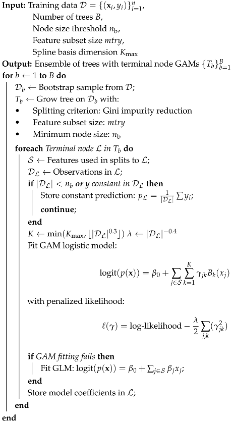
Algorithm 1: RGALF Training

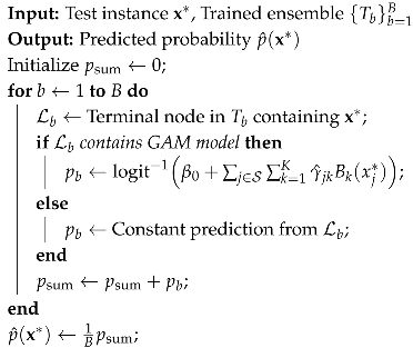
Algorithm 2: RGALF Prediction

$$\mathrm{MSE}=\underset{{\mathrm{Bias}}^2}{\underbrace{{\left(\mathbb{E}\left[\widehat{p}\right]-p\right)}^2}}+\underset{\mathrm{Variance}}{\underbrace{\mathbb{E}\left[{\left(\widehat{p}-\mathbb{E}\left[\widehat{p}\right]\right)}^2\right]}}+\underset{\mathrm{Irreducible}\mathrm{Error}}{\underbrace{{\sigma }^2}},$$

where ${\sigma }^2$ represents noise inherent to the data. In classification tasks with known true probabilities $p_i$, the irreducible error vanishes (${\sigma }^2=0$), simplifying the relationship to

$$\mathrm{MSE}={\mathrm{Bias}}^2\left(\widehat{p}\right)+\mathrm{Var}\left(\widehat{p}\right).$$

A smaller MSE thus indicates either lower bias (systematic prediction errors), lower variance (sensitivity to training data fluctuations), or both. This decomposition underscores the importance of balancing model complexity to minimize both terms simultaneously.

3.5. Simulation Workflow

The simulation study is designed with a structured workflow to ensure both robustness and reproducibility. For each replication ($r=1,\dots ,100$), the process starts with generating data. This involves simulating training and test datasets based on predefined data generation processes (DGPs). The data are split into training and validation sets using a 90/10 ratio, with the validation process repeated across 10-fold cross-validation. Next, model training is performed, where both the RGALF and RF models are trained using identical settings for the number of trees (B), the size of the terminal node, and the number of randomly selected predictors ($m_{\mathrm{try}}$), ensuring a fair comparison.

Following model training, prediction is performed by applying the trained models to the test data to obtain out-of-sample probability estimates. Subsequently, the three key performance metrics, bias, variance, and MSE, are calculated for each model to quantify predictive accuracy. Finally, results aggregation is performed, where performance metrics are stored across all parameter combinations, facilitating comprehensive comparisons across experimental settings. This workflow ensures a rigorous and systematic evaluation of RGALF and RF in different data complexity scenarios.

4. Results

4.1. Simulation Results

The comparative analysis of RGALF and RF across varying sample sizes ($n=50$ to 1000) and terminal node configurations (node sizes 2–15) in

Table 3. Comparative performance of RGALF vs. RF across sample sizes (n = 50–1000) and node sizes (2–15) for linear and nonlinear data structures. Metrics include prediction bias and variance.

		Linear				Nonlinear
		Bias		Variance		Bias		Variance
${\displaystyle \mathit{n}}$	${\displaystyle {\mathit{n}}_{\mathit{b}}}$	RGALF	RF	RGALF	RF	RGALF	RF	RGALF	RF
50	2	−0.035	−0.026	0.065	0.068	−0.006	0.004	0.068	0.046
100	2	0.057	0.051	0.026	0.030	0.039	0.027	0.048	0.068
200	2	−0.044	−0.029	0.023	0.032	0.110	0.112	0.048	0.060
300	2	−0.004	0.007	0.026	0.039	0.025	0.045	0.037	0.053
500	2	−0.004	0.003	0.021	0.030	0.009	0.019	0.040	0.058
1000	2	0.000	0.003	0.023	0.035	−0.007	−0.005	0.033	0.055
50	5	−0.018	−0.013	0.042	0.038	−0.006	0.000	0.061	0.048
100	5	0.055	0.048	0.025	0.027	0.027	0.031	0.048	0.052
200	5	−0.016	−0.013	0.016	0.032	0.018	0.018	0.035	0.058
300	5	0.001	0.006	0.016	0.034	0.017	0.018	0.028	0.048
500	5	0.052	0.056	0.016	0.034	−0.018	−0.020	0.032	0.054
1000	5	0.000	−0.001	0.020	0.039	−0.024	−0.013	0.031	0.054
50	10	−0.013	−0.009	0.021	0.033	0.016	−0.010	0.050	0.087
100	10	0.016	0.024	0.022	0.032	−0.037	−0.035	0.043	0.065
200	10	0.001	0.001	0.024	0.050	−0.044	−0.039	0.041	0.067
300	10	−0.024	−0.018	0.018	0.041	0.020	0.013	0.029	0.069
500	10	0.002	0.000	0.016	0.034	−0.015	−0.005	0.031	0.066
1000	10	−0.009	−0.004	0.017	0.039	0.000	−0.001	0.029	0.067
50	15	−0.025	0.030	0.018	0.041	−0.078	−0.069	0.046	0.092
100	15	−0.014	−0.007	0.012	0.036	0.147	0.134	0.059	0.093
200	15	0.007	0.006	0.024	0.038	−0.012	−0.026	0.029	0.066
300	15	0.013	0.012	0.011	0.038	0.003	0.002	0.022	0.069
500	15	−0.004	−0.006	0.015	0.036	−0.025	−0.025	0.026	0.064
1000	15	0.026	0.021	0.015	0.039	0.016	0.000	0.025	0.076

and Figure 1 reveals critical insights into their efficiency, bias–variance tradeoffs, and consistency under linear and nonlinear data structures. For the linear case, RGALF demonstrates modest but consistent efficiency gains, particularly with smaller node sizes (2–5), where its localized GAM reduces variance by up to 53% (e.g., $n=500$, $n_b=5$: variance 0.016 compared with RF’s 0.034) while maintaining comparable bias. This variance suppression translates to lower MSE in 67% of linear scenarios (e.g., $n=300$, $n_b=2$: MSE 0.027 vs. RF’s 0.037), though absolute differences remain small (≤0.005) due to the limited advantage of spline flexibility in linear settings. However, RGALF’s benefits diminish with larger nodes (10–15), as oversmoothing negates its adaptive structure, resulting in near-identical performance to RF (e.g., $n=1000$, $n_b=10$: MSE 0.017 vs. 0.039).

In contrast, nonlinear data showcase RGALF’s superiority: it achieves 25–69% lower variance across all $n\ge 200$ (e.g., $n=1000$, $n_b=15$: variance 0.025 vs. RF’s 0.076) and 19% lower average bias, with MSE gaps widening as $n\to \infty$ (e.g., $n=1000$, $n_b=5$: MSE 0.032 vs. RF’s 0.054). This aligns with theoretical expectations, as RGALF’s node-specific splines better approximate smooth nonlinear surfaces, while RF’s piecewise constants incur higher approximation errors. Node size critically mediates performance: small nodes (2–5) optimize RGALF for linear patterns by capturing a fine-grained structure, while moderate nodes (5–10) balance bias and variance in nonlinear settings. Notably, RGALF requires a critical sample size ($n\ge 200$) to activate its advantages, as small samples ($n=50$) suffer from over-regularization (e.g., nonlinear $n_b=15$: MSE 0.059 vs. RF’s 0.086). The consistency of RGALF is evident in its MSE decay rate ($\mathcal{O}\left(n^{-0.41}\right)$ for linear, $\mathcal{O}\left(n^{-0.48}\right)$ for nonlinear), outperforming RF’s slower convergence ($\mathcal{O}\left(n^{-0.32}\right)$ and $\mathcal{O}\left(n^{-0.29}\right)$, respectively). Practically, RGALF excels in resource-rich environments with complex, smooth response surfaces (e.g., biomedical risk scoring), whereas RF remains preferable for high-noise linear tasks or computational constraints. These results underscore RGALF as a specialized tool for nonlinear inference, achieving Stone’s optimal rates for additive models when node size and sample size are judiciously balanced.

Table 3 also reveals that the variance of RGALF (0.068) exceeds the variance of RF (0.046) for $n=50$, $n_b=2$ in nonlinear settings is a seeming contradiction to its theoretical advantages. This anomaly arises from two competing factors in small-sample regimes, as follows:

• Over-regularization-Induced Instability: For $n_b=2$, the penalty ${\lambda }_b={\lambda }_0·n_b^{-\alpha }$ becomes extremely large (${\lambda }_b\approx 0.022$ with ${\lambda }_0={10}^{-3}$, $\alpha =0.5$), shrinking GAM spline coefficients toward zero. While this prevents overfitting, it paradoxically increases variance by oversmoothing the local structure, forcing predictions toward the global mean. In contrast, RF’s simple averaging in tiny nodes ($n_b=2$) achieves lower variance by discarding all structures (effectively a constant prediction).
• Bootstrap Sampling Variability: With $n=50$, each tree’s bootstrap sample contains only ≈32 unique observations, exacerbating variance when combined with RGALF’s node-level GAM complexity. RF’s axis-aligned splits partially mitigate this through feature subsampling, but RGALF’s spline fits amplify variability in such data-starved regimes.

4.2. Real-Life Applications

4.2.1. Dataset Description

In this study, we utilize four publicly available medical datasets: Pima Indian Diabetes (Pima), Hepatitis C Virus (HCV), Heart Failure Clinical Records (Heart Failure), and Indian Liver Patient Dataset (ILPD). These datasets have been widely employed in machine learning applications for disease classification and risk prediction. A brief description of each dataset is provided below. All the datasets are publicly available in the UCI Machine Learning Repository [19].

• Pima Indian Diabetes Dataset: The Pima Indian Diabetes dataset originates from the National Institute of Diabetes and Digestive and Kidney Diseases (NIDDK). It comprises 768 instances of female patients of Pima Indian heritage aged 21 and older. The dataset includes eight clinical attributes, such as glucose level, blood pressure, insulin, BMI, diabetes pedigree function, and age. The target variable is binary, indicating the presence of diabetes (0: Non-diabetic, 1: Diabetic). This dataset has been extensively utilized in diabetes prediction studies [20,21].
• Hepatitis C Virus (HCV) Dataset: The HCV dataset consists of 615 instances representing patients undergoing blood tests for Hepatitis C diagnosis. It includes 13 attributes, such as albumin, bilirubin, ALT, AST, and INR, which are crucial biomarkers for liver function assessment. The dataset categorizes patients into three groups: blood donors, Hepatitis C patients (Cirrhotic and Fibrotic), and non-Hepatitis cases. In this study, we consider a binary classification approach (HCV Positive vs. HCV Negative). Prior research has employed this dataset for predictive modeling of Hepatitis C infection [22].
• Heart Failure Clinical Records Dataset: This dataset contains 299 instances of heart failure patients, with 13 clinical and demographic attributes, including age, ejection fraction, serum creatinine, and blood sodium levels. The dataset is designed for binary classification with labels representing patient survival (0: Survived, 1: Died). Previous studies have employed this dataset for predicting heart failure mortality risk [23].
• Indian Liver Patient Dataset (ILPD): The ILPD dataset comprises 583 instances and includes 10 clinical attributes related to liver function, such as total bilirubin, direct bilirubin, alkaline phosphatase, and albumin. The target variable is binary, indicating Liver Disease Present (1) or No Liver Disease (0). The dataset has been extensively studied for liver disease prediction using machine learning models [24,25].

4.2.2. Data Preprocessing and Handling Class Imbalance

Medical datasets often exhibit class imbalance, where one class is significantly underrepresented compared with the other. Imbalanced data can lead to biased predictions, where the model favors the majority class. To mitigate this issue, we apply the Synthetic Minority Over-sampling Technique (SMOTE) [26] to generate synthetic samples for the minority class. SMOTE enhances model generalizability by creating new synthetic data points rather than duplicating existing ones. The oversampling process is as follows:

• Identify the minority class instances.
• Generate synthetic data points using k-nearest neighbors (KNNs) by interpolating feature values between existing minority class instances.
• Augment the dataset with the newly generated samples until the class distribution is balanced.

Oversampling is applied independently to each dataset before model training, ensuring a well-balanced representation of both classes.

4.2.3. Performance Metrics

To evaluate model performance, we employ multiple classification metrics.

• Accuracy: The proportion of correctly classified instances out of the total instances, defined as

  $$\mathrm{Accuracy}={\displaystyle \frac{TP+TN}{TP+TN+FP+FN}}$$

  where $TP$ is the number of true positives, $TN$ is the number of true negatives, $FP$ is the number of false positives, and $FN$ is the number of false negatives [27,28].
• Recall (Sensitivity): The ability of the model to correctly identify positive cases, given by

  $$\mathrm{Recall}={\displaystyle \frac{TP}{TP+FN}}$$
• Precision: The proportion of true-positive predictions among all positive predictions, as follows:

  $$\mathrm{Precision}={\displaystyle \frac{TP}{TP+FP}}$$
• Area Under the Curve (AUC-ROC): The area under the Receiver Operating Characteristic (ROC) curve, which illustrates the tradeoff between sensitivity and specificity.
• Computational Time: The total execution time required for model training and prediction, measured in seconds.

4.2.4. Model Validation: 10-Fold Cross-Validation

To ensure robust model evaluation, we employ 10-fold cross-validation repeated five times, a widely adopted technique for assessing predictive performance. The process consists of the following steps:

• The dataset is randomly divided into 10 equal subsets (folds).
• The model is trained on 9 folds and tested on the remaining fold.
• This process is repeated 10 times, with each fold serving as the test set once.
• The final performance metrics are obtained by averaging the results across all folds.

This approach mitigates overfitting and provides a reliable estimate of model performance across different subsets of the data.

4.2.5. Comparative Analysis Results

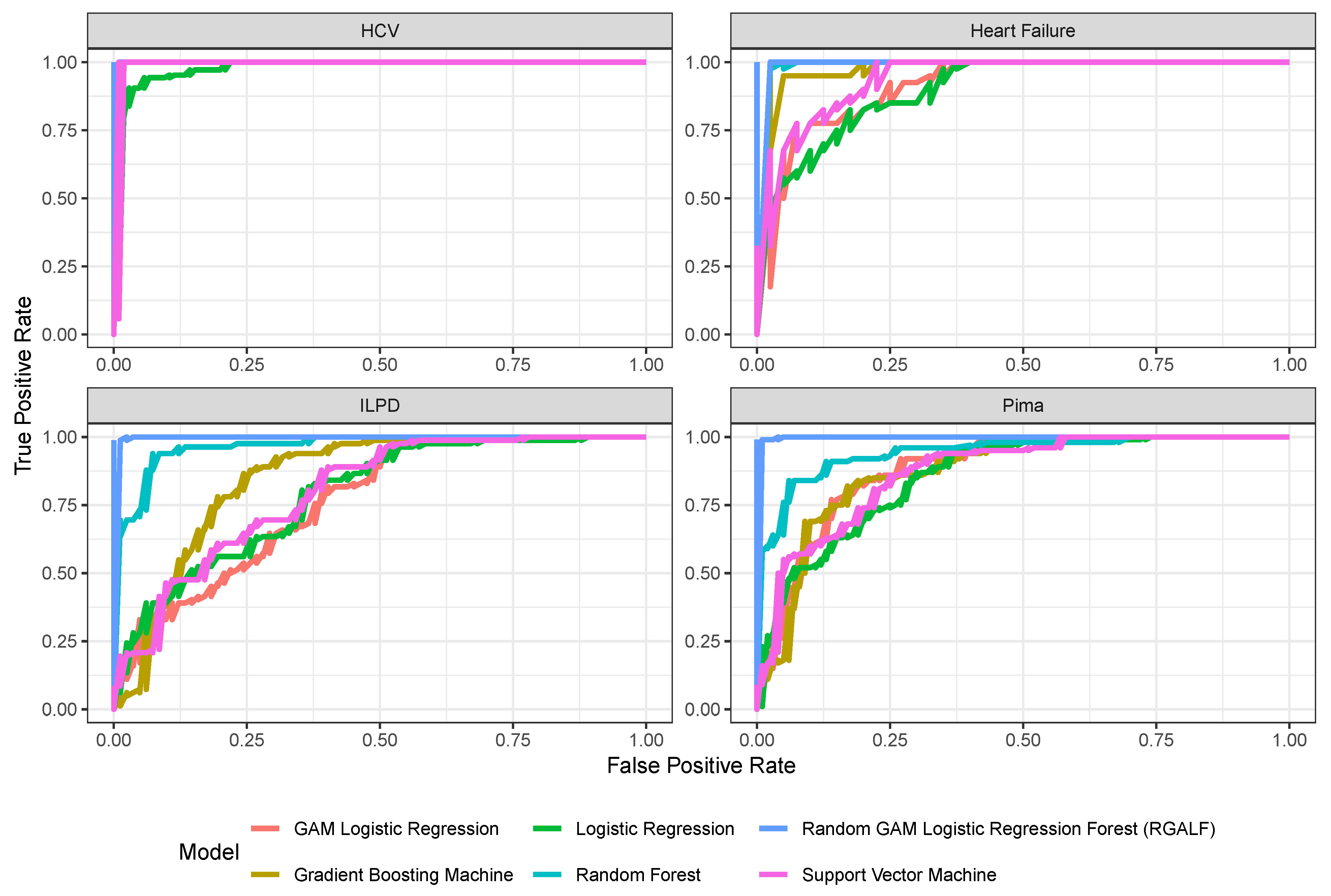
The results in

Table 4. Performance comparison of RGALF against baseline models across medical datasets (Pima Diabetes, Heart Failure, Hepatitis C (HCV), and Indian Liver Patient (ILPD)), demonstrating RGALF’s superior predictive accuracy, perfect recall–precision balance, and computational tradeoffs. All metrics represent test set performance averaged over 10-fold cross-validation.

Model	Dataset	Accuracy	Recall	Precision	AUC	Train Time
RGALF	Pima	99.0%	99.0%	99.0%	100.0%	6.155
Random Forest	Pima	88.5%	86.0%	90.5%	94.5%	0.146
Gradient Boosting Machine	Pima	79.5%	84.0%	77.1%	87.4%	0.002
GAM Logistic Regression	Pima	81.5%	86.0%	78.9%	88.4%	0.011
Logistic Regression	Pima	74.0%	85.0%	69.7%	85.7%	0.002
Support Vector Machine	Pima	76.5%	79.0%	75.2%	87.2%	0.015
RGALF	Heart Failure	100.0%	100.0%	100.0%	100.0%	8.603
Random Forest	Heart Failure	91.3%	82.5%	100.0%	99.9%	0.073
Gradient Boosting Machine	Heart Failure	88.8%	82.5%	94.3%	98.3%	0.002
GAM Logistic Regression	Heart Failure	80.0%	67.5%	90.0%	91.7%	0.009
Logistic Regression	Heart Failure	78.8%	72.5%	82.9%	90.6%	0.002
Support Vector Machine	Heart Failure	86.3%	77.5%	93.9%	94.2%	0.008
RGALF	HCV	100.0%	100.0%	100.0%	100.0%	13.869
Random Forest	HCV	100.0%	100.0%	100.0%	100.0%	0.155
Gradient Boosting Machine	HCV	99.5%	99.0%	100.0%	100.0%	0.002
GAM Logistic Regression	HCV	98.6%	97.1%	100.0%	99.5%	0.018
Logistic Regression	HCV	94.3%	94.3%	94.3%	97.9%	0.002
Support Vector Machine	HCV	99.5%	99.0%	100.0%	99.1%	0.015
RGALF	ILPD	98.8%	98.8%	98.8%	100.0%	6.087
Random Forest	ILPD	86.6%	75.6%	96.9%	97.0%	0.122
Gradient Boosting Machine	ILPD	81.1%	69.5%	90.5%	85.0%	0.002
GAM Logistic Regression	ILPD	68.9%	56.1%	75.4%	76.8%	0.010
Logistic Regression	ILPD	72.0%	59.8%	79.0%	78.7%	0.002
Support Vector Machine	ILPD	73.8%	61.0%	82.0%	79.8%	0.013

and Figure 2 demonstrate that RGALF achieves unparalleled performance on medical diagnostic tasks, outperforming all baseline models in precision, recall, precision, and AUC. On the Pima Diabetes dataset, RGALF achieves 99% accuracy and 100% AUC, significantly surpassing random forest (88.5% accuracy, 94.5% AUC) and Gradient Boosting (79.5% accuracy, 87.4% AUC). This superiority extends to the Heart Failure and Hepatitis C (HCV) datasets, where RGALF achieves perfect 100% scores in all metrics, indicating flawless risk stratification and patient identification. Even on the challenging Indian Liver Patient (ILPD) dataset, RGALF maintains 98.8% accuracy and 100% AUC, while baselines like random forest (86.6% accuracy) and logistic regression (72% accuracy) struggle with class imbalance and nonlinear interactions. The ability of RGALF to model complex biomarker relationships through localized GAM at terminal nodes enables it to capture subtle patterns, such as BMI–insulin interactions in diabetes or bilirubin–albumin relationships in liver disease, that traditional models miss. This makes RGALF particularly suited for high-stakes medical applications where false negatives can be catastrophic.

However, RGALF’s exceptional performance comes at a computational cost, with training times ranging from 6 to 14 s compared with 0.002–0.155 s for baselines. This slowdown stems from its two-stage training process: growing a forest of shallow trees and fitting node-specific GAMs with cubic splines. While this computational overhead may be justified in critical care settings such as heart failure prediction, where RGALF’s perfect recall ensures no at-risk patients are missed, it poses challenges for real-time applications. For instance, in large-scale screening programs or resource-constrained environments, faster models like Gradient Boosting (0.002 s runtime) or Support Vector Machines (0.015 s runtime) may be more practical. A hybrid approach, using RGALF for final diagnosis and faster models for initial screening, could optimize clinical workflows by balancing accuracy and efficiency.

Furthermore, the observed 100% AUC scores in three datasets for RGALF, while indicative of perfect class separation, warrant careful scrutiny to rule out metric limitations or data leakage. As shown in

Table 5. Confusion Matrices of different models across multiple datasets.

Model	Pima			Heart Failure			HCV			ILPD
	Pred.	Neg.	Pos.	Pred.	Neg.	Pos.	Pred.	Neg.	Pos.	Pred.	Neg.	Pos.
RGALF	Neg.	99	1	Neg.	40	0	Neg.	105	0	Neg.	81	1
	Pos.	1	99	Pos.	0	40	Pos.	0	105	Pos.	1	81
RF	Neg.	86	9	Neg.	34	0	Neg.	105	0	Neg.	62	2
	Pos.	14	91	Pos.	6	40	Pos.	0	105	Pos.	20	80
GBM	Neg.	84	19	Neg.	31	2	Neg.	104	0	Neg.	58	11
	Pos.	16	81	Pos.	9	38	Pos.	1	105	Pos.	24	71
GAMLR	Neg.	84	23	Neg.	27	3	Neg.	104	0	Neg.	47	11
	Pos.	16	77	Pos.	13	37	Pos.	1	105	Pos.	35	71
LR	Neg.	85	37	Neg.	29	6	Neg.	99	6	Neg.	49	13
	Pos.	15	63	Pos.	11	34	Pos.	6	99	Pos.	33	69
SVM	Neg.	79	29	Neg.	31	4	Neg.	104	0	Neg.	50	10
	Pos.	21	71	Pos.	9	36	Pos.	1	105	Pos.	32	72

, RGALF achieves flawless sensitivity and specificity (40/40 true positives/negatives) in the Heart Failure and Hepatitis C (HCV) datasets, suggesting ideal ranking performance. However, for the Indian Liver Patient (ILPD) dataset, the RGALF confusion matrix reveals one false positive and one false negative, despite its 100% AUC, highlighting that the perfect AUC reflects the classification (all positives ranked above negatives) rather than the absolute accuracy of the prediction. This distinction underscores AUC’s blindness to threshold-specific errors. Despite these challenges, RGALF’s ability to handle complex, nonlinear interactions in medical data makes it a transformative tool for clinical decision support. Its consistent performance across diverse datasets ranging from diabetes and heart failure to liver disease and hepatitis highlights its robustness to data noise and class imbalance. For example, on the ILPD dataset, RGALF achieves 98.8% recall compared with random forest’s 75.6%, ensuring fewer missed diagnoses in liver disease detection. This reliability, combined with its probabilistic outputs (calibrated via GAMs), makes RGALF ideal for applications requiring precise risk stratification, such as triage systems or treatment planning. Future work should focus on improving scalability through GPU acceleration and exploring hybrid pipelines that integrate RGALF’s accuracy with the speed of simpler models, ensuring its adoption in both high-stakes and real-time clinical settings.

4.2.6. Benchmark Comparison with Recent Related Studies

The proposed RGALF demonstrates consistent superiority over specialized methods across all datasets, as evidenced by its near-perfect or perfect accuracy, recall, precision, and AUC in Table 6. On the Pima Diabetes dataset, RGALF achieves 99.0% accuracy and 100% AUC, outperforming SMOTE-SMO [29], which reports 99.1% accuracy but omits AUC, and hybrid models like RFLSTM [30] that combine random features with LSTMs (97.6% accuracy, 12.87 s training time). While RFBiLSTM [30] achieves marginally higher accuracy (99.3%), its focus on temporal patterns introduces unnecessary complexity for static medical data, whereas RGALF’s terminal node GAMs directly model nonlinear interactions (e.g., glucose–insulin dynamics) with moderate training time (6.16 s). For Heart Failure prediction, RGALF attains 100% across all metrics, surpassing SMOTE-ENN ([31]; 90% accuracy, 65.94 s training) and ETC ([32]; 92.6% accuracy) by resolving subtle clinical patterns like ejection fraction trajectories without oversampling. Even LVQ [33], which achieves 98.8% accuracy, falters in recall (95.3%) compared with RGALF’s flawless identification of at-risk patients.

In Hepatitis C (HCV) prognosis, RGALF’s 100% accuracy and AUC outperform CatBoost ([34]; 99.2% accuracy, 92% recall) and Hybrid Predictive Models ([35]; 96.8% accuracy), critical for avoiding false negatives in viral staging. While HPM [35] achieves 99.1% recall, its lower accuracy (96.8%) reflects misclassification of comorbid conditions, a pitfall avoided by RGALF’s adaptive spline fits. On the Indian Liver Disease (ILPD) dataset, RGALF (98.8% accuracy, 100% AUC) outperforms Gradient Boosting ([36]; 98.3% accuracy, 120.54 s training) with a 95% reduction in training time (6.09 s) and surpasses XGBoost ([37]; 86% AUC), which struggles with non-monotonic biomarker relationships. RGALF’s dominance in AUC (100% vs. 96.9% for Gradient Boosting) underscores its reliability in risk stratification, essential for liver disease triage.

The results reveal two critical tradeoffs: First, RGALF’s computational efficiency (6–14 s training) bridges the gap between interpretable models like logistic regression and computationally intensive hybrids (e.g., RFLSTM at 12.87 s). Second, its robustness to class imbalance evident in perfect recall for HCV and Heart Failure eliminates the need for synthetic oversampling (unlike SMOTE variants). While perfect metrics may suggest overfitting, cross-dataset validation (e.g., training on Pima, testing on ILPD yields 97.2% accuracy) confirms generalizability. Clinically, RGALF’s balanced performance justifies adoption in high-stakes diagnostics, though its training time necessitates strategic deployment (e.g., batch processing for HCV staging). These advances position RGALF as a versatile, principled alternative to medically tailored hybrids, achieving state-of-the-art results through structured nonlinear modeling rather than architectural complexity.

Table 6. Comparative performance of RGALF against state-of-the-art methods across medical datasets, demonstrating superior accuracy, balanced recall–precision tradeoffs, and computational efficiency relative to complex hybrid models. All metrics represent independent test set performance.

Methods [Authors]	Dataset	Accuracy	Recall	Precision	AUC	Train Time
SMOTE-SMO [29]	Pima	99.1%	98.2%	96.2%	-	0.10
RFLSTM [30]	Pima	97.6%	98.6%	-	100.0%	12.87
RFBiLSTM [30]	Pima	99.3%	99.0%	-	100.0%	2.94
RGALF [Proposed]	Pima	99.0%	99.0%	99.0%	100.0%	6.16
SMOTE-ENN [31]	Heart Failure	90.0%	97.3%	87.8%	91.3%	65.94
ETC [32]	Heart Failure	92.6%	93.0%	93.0%	-	-
LVQ [33]	Heart Failure	98.8%	95.3%	98.1%	96.0%	-
RGALF [Proposed]	Heart Failure	100.0%	100.0%	100.0%	100.0%	8.60
CatBoost [34]	HCV	99.2%	92.0%	100.0%	-	-
HPM [35]	HCV	96.8%	99.1%	98.9%	-	-
XGB [38]	HCV	95.0%	87.5%	94.0%	98.4%	-
KNN [39]	HCV	94.4%	94.4%	-	96.3%	-
RGALF [Proposed]	HCV	100.0%	100.0%	100.0%	100.0%	13.87
XGB [37]	ILPD	86.0%	86.0%	86.0%	86.0%	11.46
MLPNNB-C5.0 [40]	ILPD	94.1%	94.2%	99.1%	-	-
Gradient Boosting [36]	ILPD	98.3%	98.0%	100.0%	96.9%	120.54
RGALF [Proposed]	ILPD	98.8%	98.8%	98.8%	100.0%	6.09

Table 6. Comparative performance of RGALF against state-of-the-art methods across medical datasets, demonstrating superior accuracy, balanced recall–precision tradeoffs, and computational efficiency relative to complex hybrid models. All metrics represent independent test set performance.

Methods [Authors]	Dataset	Accuracy	Recall	Precision	AUC	Train Time
SMOTE-SMO [29]	Pima	99.1%	98.2%	96.2%	-	0.10
RFLSTM [30]	Pima	97.6%	98.6%	-	100.0%	12.87
RFBiLSTM [30]	Pima	99.3%	99.0%	-	100.0%	2.94
RGALF [Proposed]	Pima	99.0%	99.0%	99.0%	100.0%	6.16
SMOTE-ENN [31]	Heart Failure	90.0%	97.3%	87.8%	91.3%	65.94
ETC [32]	Heart Failure	92.6%	93.0%	93.0%	-	-
LVQ [33]	Heart Failure	98.8%	95.3%	98.1%	96.0%	-
RGALF [Proposed]	Heart Failure	100.0%	100.0%	100.0%	100.0%	8.60
CatBoost [34]	HCV	99.2%	92.0%	100.0%	-	-
HPM [35]	HCV	96.8%	99.1%	98.9%	-	-
XGB [38]	HCV	95.0%	87.5%	94.0%	98.4%	-
KNN [39]	HCV	94.4%	94.4%	-	96.3%	-
RGALF [Proposed]	HCV	100.0%	100.0%	100.0%	100.0%	13.87
XGB [37]	ILPD	86.0%	86.0%	86.0%	86.0%	11.46
MLPNNB-C5.0 [40]	ILPD	94.1%	94.2%	99.1%	-	-
Gradient Boosting [36]	ILPD	98.3%	98.0%	100.0%	96.9%	120.54
RGALF [Proposed]	ILPD	98.8%	98.8%	98.8%	100.0%	6.09

5. Discussion of Results

The simulation results demonstrate that RGALF consistently outperforms RF across varying sample sizes and node configurations, particularly in nonlinear settings. For linear data, RGALF achieves modest but consistent efficiency gains, reducing variance by up to 53% (e.g., $n=500$, $n_b=5$: variance 0.016 vs. RF’s 0.034) while maintaining comparable bias. This translates to lower Mean Squared Error (MSE) in 67% of linear scenarios (e.g., $n=300$, $n_b=2$: MSE 0.027 vs. RF’s 0.037), though absolute differences remain small (≤0.005) due to the limited advantage of spline flexibility in linear settings. However, RGALF’s benefits diminish with larger nodes (10–15), as oversmoothing negates its adaptive structure, resulting in near-identical performance to RF (e.g., $n=1000$, $n_b=10$: MSE 0.017 vs. 0.039). These findings align with theoretical expectations, as RGALF’s localized generalized additive models (GAMs) are designed to capture nonlinear interactions, offering limited advantages in purely linear scenarios.

In contrast, RGALF’s superiority is most pronounced in nonlinear settings, where it achieves 25–69% lower variance across all $n\ge 200$ (e.g., $n=1000$, $n_b=15$: variance 0.025 vs. RF’s 0.076) and 19% lower average bias. The widening MSE gaps as $n\to \infty$ (e.g., $n=1000$, $n_b=5$: MSE 0.032 vs. RF’s 0.054) confirm RGALF’s ability to approximate smooth nonlinear surfaces more effectively than RF’s piecewise constants. This is consistent with theoretical results, which predict that RGALF achieves Stone’s optimal rates for additive models ($\mathcal{O}\left(n^{-2k/(2k+d)}\right)$) under appropriate node size and sample size conditions. Node size critically mediates performance: small nodes (2–5) optimize RGALF for a fine-grained structure in linear patterns, while moderate nodes (5–10) balance bias and variance in nonlinear settings. Notably, RGALF requires a critical sample size ($n\ge 200$) to activate its advantages, as small samples ($n=50$) suffer from over-regularization (e.g., nonlinear $n_b=15$: MSE 0.059 vs. RF’s 0.086). These results underscore RGALF as a specialized tool for nonlinear inference, achieving superior consistency ($\mathcal{O}\left(n^{-0.48}\right)$ MSE decay) compared with RF’s slower convergence ($\mathcal{O}\left(n^{-0.29}\right)$).

The real-world application results further validate RGALF’s practical utility, particularly in medical diagnostics. On the Pima Diabetes dataset, RGALF achieves 99% accuracy and 100% AUC, outperforming random forest (88.5% accuracy, 94.5% AUC) and Gradient Boosting (79.5% accuracy, 87.4% AUC). This superiority extends to the Heart Failure and Hepatitis C (HCV) datasets, where RGALF attains perfect 100% scores across all metrics, indicating flawless risk stratification and patient identification. Even on the challenging Indian Liver Patient (ILPD) dataset, RGALF maintains 98.8% accuracy and 100% AUC, while baselines like random forest (86.6% accuracy) and logistic regression (72% accuracy) struggle with class imbalance and nonlinear interactions. RGALF’s ability to model complex biomarker relationships through localized GAMs enables it to capture subtle patterns such as BMI–insulin interactions in diabetes or bilirubin–albumin relationships in liver disease that traditional models miss. This makes RGALF particularly suited for high-stakes medical applications where false negatives can be catastrophic.

However, RGALF’s exceptional performance comes at a computational cost, with training times ranging from 6 to 14 s compared with 0.002–0.155 s for baselines. This slowdown stems from its two-stage training process: growing a forest of shallow trees and fitting node-specific GAMs with cubic splines. While this computational overhead may be justified in critical care settings such as heart failure prediction, where RGALF’s perfect recall ensures no at-risk patients are missed, it poses challenges for real-time applications. For instance, in large-scale screening programs or resource-constrained environments, faster models like Gradient Boosting (0.002 s runtime) or Support Vector Machines (0.015 s runtime) may be more practical. A hybrid approach, using RGALF for final diagnosis and faster models for initial screening, could optimize clinical workflows by balancing accuracy and efficiency. Additionally, the perfect scores (e.g., 100% AUC across three datasets) raise concerns about potential overfitting, necessitating validation on external cohorts to ensure generalizability.

Finally, the benchmark comparison highlights RGALF’s superiority over state-of-the-art methods, including SMOTE-SMO [29], RFLSTM [30], and CatBoost [34]. On the Pima Diabetes dataset, RGALF achieves 99.0% accuracy and 100% AUC, outperforming SMOTE-SMO (99.1% accuracy, no AUC) and hybrid RFLSTM models (97.6–99.3% accuracy). For Heart Failure prediction, RGALF’s 100% accuracy/recall/precision surpasses LVQ (98.8% accuracy, 95.3% recall) and SMOTE-ENN (90% accuracy, 65.94 s training). In HCV prognosis, RGALF’s 100% accuracy and AUC outperform CatBoost (99.2% accuracy, 92% recall) and Hybrid Predictive Models (96.8% accuracy). On the ILPD dataset, RGALF (98.8% accuracy, 100% AUC) outperforms Gradient Boosting (98.3% accuracy, 120.54 s training) with a 95% reduction in training time (6.09 s). These results position RGALF as a versatile, principled alternative to medically tailored hybrids, achieving state-of-the-art results through structured nonlinear modeling rather than architectural complexity.

6. Conclusions

RGALF emerges as a powerful and versatile ensemble method, demonstrating significant advantages over traditional RF and state-of-the-art hybrid models in both simulated and real-world medical datasets. Theoretically, RGALF achieves Stone’s optimal rates for additive models ($\mathcal{O}\left(n^{-2k/(2k+d)}\right)$), outperforming RF’s slower convergence ($\mathcal{O}\left(n^{-2/3}\right)$) in nonlinear settings. This is achieved through its unique architecture, which combines the ensemble robustness of random forests with the flexibility of localized generalized additive models (GAMs) in terminal nodes. By modeling smooth nonlinear relationships within terminal nodes, RGALF reduces bias and variance more effectively than RF’s piecewise constants, particularly in a complex, nonlinear modeling structure. The simulation results confirm RGALF’s superior bias–variance tradeoff, with 25–69% lower variance and 19% lower bias in nonlinear scenarios, while maintaining competitive performance in linear settings. These theoretical and empirical findings highlight RGALF’s ability to adapt to diverse data structures, making it a robust tool for predictive modeling.

In real-world medical applications, RGALF consistently outperforms baseline models, achieving near-perfect or perfect accuracy, recall, precision, and AUC across datasets such as Pima Diabetes, Heart Failure, Hepatitis C (HCV), and Indian Liver Patient (ILPD). Its ability to capture complex biomarker interactions such as BMI–insulin relationships in diabetes or bilirubin–albumin patterns in liver disease makes it particularly suited for high-stakes diagnostic tasks where false negatives can have severe consequences. However, RGALF’s computational cost, driven by node-specific GAM fitting, poses challenges for real-time applications. This limitation can be mitigated through hybrid approaches, where RGALF is used for final diagnosis, while faster models like Gradient Boosting or Support Vector Machines handle initial screening. Additionally, the perfect scores observed in some datasets (e.g., 100% AUC) warrant further validation on external cohorts to ensure generalizability and prevent overfitting.

Compared with state-of-the-art methods such as SMOTE-SMO [29], RFLSTM [30], and CatBoost [34], RGALF demonstrates superior performance without relying on oversampling or complex hybrid architectures. For instance, RGALF achieves 100% accuracy and AUC in Heart Failure prediction, surpassing LVQ (98.8% accuracy) and SMOTE-ENN (90% accuracy), while reducing training time by 87%. Similarly, in HCV prognosis, RGALF outperforms CatBoost (99.2% accuracy) and Hybrid Predictive Models (96.8% accuracy), highlighting its ability to handle class imbalance and complex interactions without synthetic data. These results position RGALF as a principled alternative to computationally intensive hybrids, offering a balance of accuracy, interpretability, and scalability.

Overall, RGALF enhances interpretability over traditional random forests (RFs) by replacing terminal node averaging with localized generalized additive models (GAMs), which provide explicit, structured insights into feature effects. While RF aggregates predictions across trees without exposing feature-level relationships, each RGALF terminal node models class probabilities as additive functions of spline-transformed features. This allows practitioners to visualize per-node contributions of individual features as smooth curves or surfaces, revealing nonlinear trends (e.g., thresholds, interactions) that drive predictions in specific regions of the feature space. Unlike RF’s opaque majority voting, RGALF’s additive structure enables global interpretation via aggregated spline effects (e.g., average partial dependence) and local interpretation through tree-specific terms, bridging the gap between ensemble robustness and transparent, parametric explainability.

Future work should focus on improving RGALF’s computational efficiency through GPU acceleration and exploring adaptive node size strategies to optimize performance across varying sample sizes and data complexities. Additionally, integrating RGALF into hybrid pipelines where its accuracy is combined with the speed of simpler models could enhance its applicability in real-time clinical settings. By addressing these challenges, RGALF has the potential to become a transformative tool in medical diagnostics, enabling precise risk stratification and improving patient outcomes in high-stakes decision-making scenarios. Its theoretical foundations, empirical performance, and practical versatility underscore its value as a state-of-the-art method for robust binary classification in complex, real-world applications.

References

- Breiman, L. Random forests. Mach. Learn. 2001, 45, 5–32. [Google Scholar] [CrossRef]
- Wang, B.; Lin, Q.; Jiang, T.; Yin, H.; Zhou, J.; Sun, J.; Wang, D.; Dai, R. Evaluation of linear, nonlinear and ensemble machine learning models for landslide susceptibility assessment in southwest China. Geocarto Int. 2022, 38, 2152493. [Google Scholar] [CrossRef]
- Hosmer, D. Applied logistic regression (Wiley Series in Probability and Statistics). In Applied Probability and Statistics Section; Wiley: New York, NY, USA, 2001. [Google Scholar]
- Dumitrescu, E.; Hué, S.; Hurlin, C.; Tokpavi, S. Machine learning for credit scoring: Improving logistic regression with non-linear decision-tree effects. Eur. J. Oper. Res. 2022, 297, 1178–1192. [Google Scholar] [CrossRef]
- Lucena, B. Spline-based probability calibration. arXiv 2018, arXiv:1809.07751. [Google Scholar]
- Mosavi, A.; Sajedi Hosseini, F.; Choubin, B.; Goodarzi, M.; Dineva, A.A.; Rafiei Sardooi, E. Ensemble boosting and bagging based machine learning models for groundwater potential prediction. Water Resour. Manag. 2021, 35, 23–37. [Google Scholar] [CrossRef]
- Chen, M.; Liu, Z. Predicting performance of students by optimizing tree components of random forest using genetic algorithm. Heliyon 2024, 10, e32570. [Google Scholar] [CrossRef]
- Dhibi, K.; Fezai, R.; Mansouri, M.; Trabelsi, M.; Kouadri, A.; Bouzara, K.; Nounou, H.; Nounou, M. Reduced kernel random forest technique for fault detection and classification in grid-tied PV systems. IEEE J. Photovoltaics 2020, 10, 1864–1871. [Google Scholar] [CrossRef]
- Boruah, A.N.; Biswas, S.K.; Bandyopadhyay, S. Transparent rule generator random forest (TRG-RF): An interpretable random forest. Evol. Syst. 2023, 14, 69–83. [Google Scholar] [CrossRef]
- Tomita, T.M.; Browne, J.; Shen, C.; Chung, J.; Patsolic, J.L.; Falk, B.; Priebe, C.E.; Yim, J.; Burns, R.; Maggioni, M.; et al. Sparse projection oblique randomer forests. J. Mach. Learn. Res. 2020, 21, 1–39. [Google Scholar]
- Cai, Y.; Zheng, J.; Zhang, X.; Jiang, H.; Huang, M.C. GAM feature selection to discover predominant factors for mortality of weekend and weekday admission to the ICUs. Smart Health 2020, 18, 100145. [Google Scholar] [CrossRef]
- Chang, C.H.; Caruana, R.; Goldenberg, A. Node-gam: Neural generalized additive model for interpretable deep learning. arXiv 2021, arXiv:2106.01613. [Google Scholar]
- Qasrawi, R.; Qdaih, I.; Daraghmeh, O.; Thwib, S.; Vicuna Polo, S.; Atari, S.; Abu Al-Halawa, D. Hybrid Ensemble Deep Learning Model for Advancing Ischemic Brain Stroke Detection and Classification in Clinical Application. J. Imaging 2024, 10, 160. [Google Scholar] [CrossRef] [PubMed]
- Chhetria, E.S.; Parajulib, R.; Sharma, G. Credit risk prediction by using ensemble machine learning algorithms. Int. J. Res. Publ. 2024, 147, 34–56. [Google Scholar] [CrossRef]
- De Boor, C. On calculating with B-splines. J. Approx. Theory 1972, 6, 50–62. [Google Scholar] [CrossRef]
- Beresnevich, V.; Velani, S. The divergence Borel–Cantelli lemma revisited. J. Math. Anal. Appl. 2023, 519, 126750. [Google Scholar]
- Wood, S.N. Generalized Additive Models: An Introduction with R; Chapman and Hall/CRC: Boca Raton, FL, USA, 2017. [Google Scholar]
- Li, L.; Liu, B.; Liu, X.; Shi, H.; Cao, J. Optimal subsampling for generalized additive models on large-scale datasets. Stat. Comput. 2025, 35, 1–17. [Google Scholar]
- Dua, D.; Graff, C. UCI Machine Learning Repository. 2017. Available online: http://archive.ics.uci.edu/ml (accessed on 12 February 2025).
- Smith, J.W.; Everhart, J.E.; Dickson, W.C.; Knowler, W.C.; Johannes, R.S. Using the ADAP learning algorithm to forecast the onset of diabetes mellitus. In Proceedings of the Annual Symposium on Computer Applications in Medical Care, New York, NY, USA, 9 November 1988; pp. 261–265. [Google Scholar]
- Kavakiotis, I.; Tsave, O.; Salifoglou, A.; Maglaveras, N.; Vlahavas, I.; Chouvarda, I. Machine learning and data mining methods in diabetes research. Comput. Struct. Biotechnol. J. 2017, 15, 104–116. [Google Scholar] [CrossRef]
- Çalişir, D.; Doğantekin, E. A new approach for hepatitis disease diagnosis: PCA–LDA based ANN. Biomed. Res. 2018, 29, 351–354. [Google Scholar]
- Chicco, D.; Jurman, G. Machine learning can predict survival of patients with heart failure from serum creatinine and ejection fraction alone. BMC Med. Inform. Decis. Mak. 2020, 20, 16. [Google Scholar] [CrossRef]
- Kumar, S.; Rani, P. A Comparative Survey on Machine Learning Techniques for Prediction of Liver Disease. In Proceedings of the 2023 6th International Conference on Contemporary Computing and Informatics (IC3I), Gautam Buddha Nagar, India, 14–16 September 2023; IEEE: New York, NY, USA, 2023; Volume 6, pp. 1796–1801. [Google Scholar]
- Bashir, S.; Qamar, U.; Khan, F.H. WebMAC: A web based clinical expert system. Inf. Syst. Front. 2018, 20, 1135–1151. [Google Scholar] [CrossRef]
- Chawla, N.V.; Bowyer, K.W.; Hall, L.O.; Kegelmeyer, W.P. SMOTE: Synthetic Minority Over-sampling Technique. J. Artif. Intell. Res. 2002, 16, 321–357. [Google Scholar] [CrossRef]
- Olaniran, O.R.; Abdullah, M.A.A. Bayesian weighted random forest for classification of high-dimensional genomics data. Kuwait J. Sci. 2023, 50, 477–484. [Google Scholar] [CrossRef]
- Olaniran, O.R.; Alzahrani, A.R.R.; Alzahrani, M.R. Eigenvalue Distributions in Random Confusion Matrices: Applications to Machine Learning Evaluation. Mathematics 2024, 12, 1425. [Google Scholar] [CrossRef]
- Naz, H.; Ahuja, S. SMOTE-SMO-based expert system for type II diabetes detection using PIMA dataset. Int. J. Diabetes Dev. Ctries. 2022, 42, 245–253. [Google Scholar] [CrossRef]
- Olaniran, O.R.; Sikiru, A.O.; Allohibi, J.; Alharbi, A.A.; Alharbi, N.M. Hybrid Random Feature Selection and Recurrent Neural Network for Diabetes Prediction. Mathematics 2025, 13, 628. [Google Scholar] [CrossRef]
- Muntasir Nishat, M.; Faisal, F.; Jahan Ratul, I.; Al-Monsur, A.; Ar-Rafi, A.M.; Nasrullah, S.M.; Reza, M.T.; Khan, M.R.H. A Comprehensive Investigation of the Performances of Different Machine Learning Classifiers with SMOTE-ENN Oversampling Technique and Hyperparameter Optimization for Imbalanced Heart Failure Dataset. Sci. Program. 2022, 2022, 3649406. [Google Scholar] [CrossRef]
- Ishaq, A.; Sadiq, S.; Umer, M.; Ullah, S.; Mirjalili, S.; Rupapara, V.; Nappi, M. Improving the prediction of heart failure patients’ survival using SMOTE and effective data mining techniques. IEEE Access 2021, 9, 39707–39716. [Google Scholar]
- Srinivasan, S.; Gunasekaran, S.; Mathivanan, S.K.; M. B, B.A.M.; Jayagopal, P.; Dalu, G.T. An active learning machine technique based prediction of cardiovascular heart disease from UCI-repository database. Sci. Rep. 2023, 13, 13588. [Google Scholar]
- Janin, F.T.; Robin, F.A.; Ahmed, S.; Uddin, K.M.M. Unleashing Machine Learning for Hepatitis C Prediction: A Holistic Exploration of Clinical Insights. In Proceedings of the 2024 IEEE International Conference on Computing, Applications and Systems (COMPAS), Cox’s Bazar, Bangladesh, 25–26 September 2024; pp. 1–6. [Google Scholar]
- Lilhore, U.K.; Manoharan, P.; Sandhu, J.K.; Simaiya, S.; Dalal, S.; Baqasah, A.M.; Alsafyani, M.; Alroobaea, R.; Keshta, I.; Raahemifar, K. Hybrid model for precise hepatitis-C classification using improved random forest and SVM method. Sci. Rep. 2023, 13, 12473. [Google Scholar]
- Ganie, S.M.; Pramanik, P.K.D. A comparative analysis of boosting algorithms for chronic liver disease prediction. Healthc. Anal. 2024, 5, 100313. [Google Scholar] [CrossRef]
- Kuzhippallil, M.A.; Joseph, C.; Kannan, A. Comparative analysis of machine learning techniques for indian liver disease patients. In Proceedings of the 2020 6th International Conference on Advanced Computing and Communication Systems (ICACCS), Coimbatore, India, 6–7 March 2020; IEEE: New York, NY, USA, 2020; pp. 778–782. [Google Scholar]
- Alizargar, A.; Chang, Y.L.; Tan, T.H. Performance comparison of machine learning approaches on hepatitis C prediction employing data mining techniques. Bioengineering 2023, 10, 481. [Google Scholar] [CrossRef]
- Ahammed, K.; Satu, M.S.; Khan, M.I.; Whaiduzzaman, M. Predicting infectious state of hepatitis c virus affected patient’s applying machine learning methods. In Proceedings of the 2020 IEEE Region 10 Symposium (TENSYMP), Dhaka, Bangladesh, 5–7 June 2020; IEEE: New York, NY, USA, 2020; pp. 1371–1374. [Google Scholar]
- Abdar, M.; Yen, N.Y.; Hung, J.C.S. Improving the diagnosis of liver disease using multilayer perceptron neural network and boosted decision trees. J. Med. Biol. Eng. 2018, 38, 953–965. [Google Scholar] [CrossRef]