Abstract
We propose a U-Net regression network model for sliced data to reconstruct a three-dimensional irregular steady-state sound field filling inhomogeneous anisotropic media. Through an innovative sliced data processing strategy, the 3D reconstruction problem is decomposed into a combination of 2D problems, thereby significantly reducing the computational cost. The designed multi-channel U-Net fully utilizes the strengths of both the encoder and decoder, exhibiting strong feature extraction and spatial detail recovery capabilities. Numerical experiments show that the model can not only effectively reconstruct the complex sound field structure containing non-convex regions, but it can also synchronously restore the spatial distribution of the media and their parameter matrix, successfully achieving the dual reconstruction of the shape and physical parameters of the steady-state sound field.
Keywords:
inverse scattering problem; 3D inhomogeneous steady-state sound field reconstruction; sliced data processing strategy; multi-channel U-Net MSC:
35R30
1. Introduction
Acoustics is an important branch of physics with a rich background of practical applications, such as in medical imaging [1], sonar detection [2], and nondestructive testing [3]. The fundamental study of acoustics centers around sound waves, which are mechanical waves that propagate in an elastic medium. The research on acoustic waves mainly includes the generation, radiation, scattering, and reception of acoustic waves, involving materials, vibration, numerical simulation, and other related fields, while continuously intersecting with emerging disciplines and new materials, resulting in a high level of complexity. The inverse problem is designed to reconstruct the information within a region when the output of that region is known. In an acoustic context, it is of great research value to invert the properties as well as the spatial distribution of the medium in the acoustic field with known information about the acoustic pressure field. Acoustic field inversion problems can usually be studied based on scattering theory, which is based on fluctuation equations to describe the propagation and scattering behavior of acoustic waves in different media. In practical applications, information about the sound field is usually obtained by measuring scattering data (such as sound pressure, sound velocity, etc.). Acoustic field inversion has a wide range of applications in medical imaging [4], geological exploration, biological recognition [5], and other fields.
Inversion methods can be divided into traditional numerical methods and modern methods based on deep learning. The traditional method is based on strict physical equations, requires fine modeling, is easily affected by model errors, and relies on regularization design. Traditional methods are difficult to choose due to the trade-off between calculation accuracy and efficiency. Traditional inversion methods based on classical mathematical and physical models mainly rely on analytical or numerical solutions of the scattered field, as well as classical optimization and inversion algorithms. These methods are usually based on physical theories such as Maxwell’s equations and invert the physical parameters of the medium by solving the corresponding transport equations. The approximation method is suitable for simple, weak scattering problems with relatively limited accuracy. The Born approximation method [6,7] is one of the earliest analytical methods proposed for reconstruction. The Rytov approximation method [8,9,10] is an improved linearization method. Unlike the Born approximation, the Rytov approximation focuses on the phase change of the wave, making it more appropriate for high-frequency wave propagation problems. Iterative optimization algorithms are effective for nonlinear problems and excel at handling complex inverse problems, though they come with high computational costs. The Newton method [11,12] and the Gauss–Newton method [13] reconstruct the physical parameters by gradually approaching the error between the measured data and the model prediction data. The Newton method is optimized based on the second derivative of the objective function, and the convergence speed is fast. The Gauss–Newton method is an enhanced version of the Newton method, which approximates the objective function by neglecting the second-order term and is well suited for nonlinear least squares problems. The Algebraic Reconstruction Technique (ART) [14] is a reconstruction method based on solving linear equations, which is suitable for discrete problems.
The numerical solution method is effective for addressing problems with complex geometries and boundary conditions, which enhances accuracy, though it comes at the expense of increased computational complexity. The finite difference method is a numerical method for solving partial differential equations. The continuous equation of the physical field is discretized into finite difference equations using numerical methods, and the distribution of the physical field on the discrete grid is solved to reconstruct the physical parameters. The method is suitable for reconstruction problems with geometric structure rules. When the geometric structure is complex, the finite element method can be used to reconstruct the physical parameters. It divides the target region into several small units and establishes local equations on each unit. Then, it solves these local equations to achieve the purpose of reconstructing the physical parameters of the target region. Like all inverse problems, acoustic field inversion based on scattering theory may also face the ill-posed problem, that is, the observation data may not uniquely inverse the characteristics of the target. In the traditional method, the ill-posed problem is solved by introducing the regularization term [15,16], but the choice of the regularization parameter is crucial for obtaining an effective solution.
In recent years, with the improvement of computer performance and the development of deep learning algorithms, scholars have begun exploring the use of deep learning methods to realize the inversion of the acoustic field. The strengths of deep learning lie in its powerful data-driven capability, nonlinear modeling capability, and the fact that it does not need to rely on rigorous physical models.
Kamilov et al. [17] proposed a nonlinear inverse scattering method that combines the iterative Born approximation with a hierarchy of artificial neural networks to develop an efficient error backpropagation algorithm for estimating the target parameters. Li et al. [18] proposed an efficient deep convolutional neural network approach and demonstrated its potential in solving the inverse scattering problem. Wei and Chen [19] proposed an induced current learning method that uses a physically-inspired convolutional neural network to solve the full-wave inverse scattering problem. The method employs a cascaded end-to-end CNN architecture with a multi-label loss function to reduce the nonlinearity of the objective function. Additionally, hopping connections are introduced to focus on learning small portions of the induced currents, which accelerates convergence and reduces the learning difficulty. Xiao et al. [20] proposed a 3D inversion method that combines the Born approximation with a 3D convolutional neural network to reconstruct inhomogeneous scatterers embedded in a layered medium. Li et al. [21] proposed a multi-channel U-Net convolutional neural network to solve the multi-frequency backscattering problem. The method yields acceptable results in a very short time and avoids the drawbacks of traditional iterative methods. Xu et al. [22] proposed an end-to-end scalable cascaded convolutional neural network approach to the inverse scattering problem. The method decomposes full-wave inversion into two parts as follows: first, it performs a linear transformation to obtain a preliminary image, and then, it reconstructs the high-resolution image using a multiresolution imaging network. Multi-resolution labeling guides the cascade network to gradually recover the high-frequency component, enhancing the network’s physical significance and interpretability while improving inversion accuracy and efficiency. Aydın et al. [23] presented a deep learning technique based on convolutional neural networks for imaging rough surfaces between two media. The paper designed and implemented two different CNN architectures to solve the inverse rough surface imaging problem. Zhang et al. [24] proposed an unfolded deep learning scheme that combines the CSI method with ResNet to solve the full-wave nonlinear inverse scattering problem. In numerical experiments, the method demonstrates advantages in stability, robustness, and reliability. Barmada et al. [25] proposed a deep learning method based on conditional variational self-encoders and convolutional neural networks to solve an inverse problem.
In addition, Puzyrev [26] presented a deep learning-based method that provided fast results without gradient computation, exploring the potential of deep learning methods in inversion. Yao et al. [27] proposed a novel deep learning method based on a convolutional encoder–decoder architecture to solve the inverse scattering problem. The numerical results demonstrate the method’s feasibility and accuracy, opening a new path for the real-time quantitative microwave imaging of high-contrast scatterers using deep learning. Ye et al. [28] introduced a noniterative method called the distortion-Born backpropagation scheme (DB-BPS) for reconstructing rough images of unknown object in inhomogeneous backgrounds to alleviate the burden of the nonlinearity and ill-posedness of the inverse scattering problem. The rough reconstruction result is used as input to the designed generative adversarial network, which outputs the fine reconstructed image of the relative permittivity. The proposed method has proven to be effective in reconstructing object embedded in inhomogeneous backgrounds and has various potential applications. Song et al. [29] proposed a two-step learning-based approach to the inverse scattering problem, using backpropagation for coarse imaging in the first step and a perceptual generative adversarial network for resolution enhancement in the second. Hu et al. [30] proposed a more generalized backscattering method based on physically informed neural networks.
Modern methods based on deep learning mostly discuss the feasibility and efficiency of the method, and there are not many examples combined with practical applications. Therefore, we propose a U-Net based regression network model for sliced data to reconstruct a three-dimensional irregular sound field filling inhomogeneous anisotropic media. It not only improves the problem of high computational complexity associated with the traditional methods, but it also successfully combines this method with practical problems. The Petrov–Galerkin finite element interface method (PGFEIM) is used to solve the acoustic field problem and obtain the initial data for the inverse problem. The method uses a consistent non-body mesh that can easily handle problems with arbitrarily complex shapes. In addition, the method is easy to program and computationally inexpensive. For three-dimensional positive and inverse problems, the amount of data is very large. Therefore, this paper proposes a processing method based on two-dimensional problems, called the slicing method. We slice the obtained initial data in different directions and reduce their dimension from three-dimensional to two-dimensional. This method transforms the reconstruction problem of the three-dimensional physical field into a combination of multiple two-dimensional problems, which greatly reduces the computational cost.
This paper is organized as follows. Section 2 briefly introduces the sound pressure field problem and the PGFEIM. In Section 3, the U-Net based regression network model for sliced data is discussed in detail. Section 4 demonstrates the performance and advantages of the proposed method through numerical experiments. Finally, conclusions are presented in Section 5.
2. Three-Dimensional Inhomogeneous Anisotropic Steady-State Sound Field
In this section, we present the numerical method for solving the steady-state acoustic field of the three-dimensional irregular region filled with inhomogeneous anisotropic media. It should be clear that the solution domains are all three-dimensional arbitrary bounded open domains, denoted as .
2.1. Mathematical Model of the Three-Dimensional Inhomogeneous Anisotropic Steady-State Sound Field
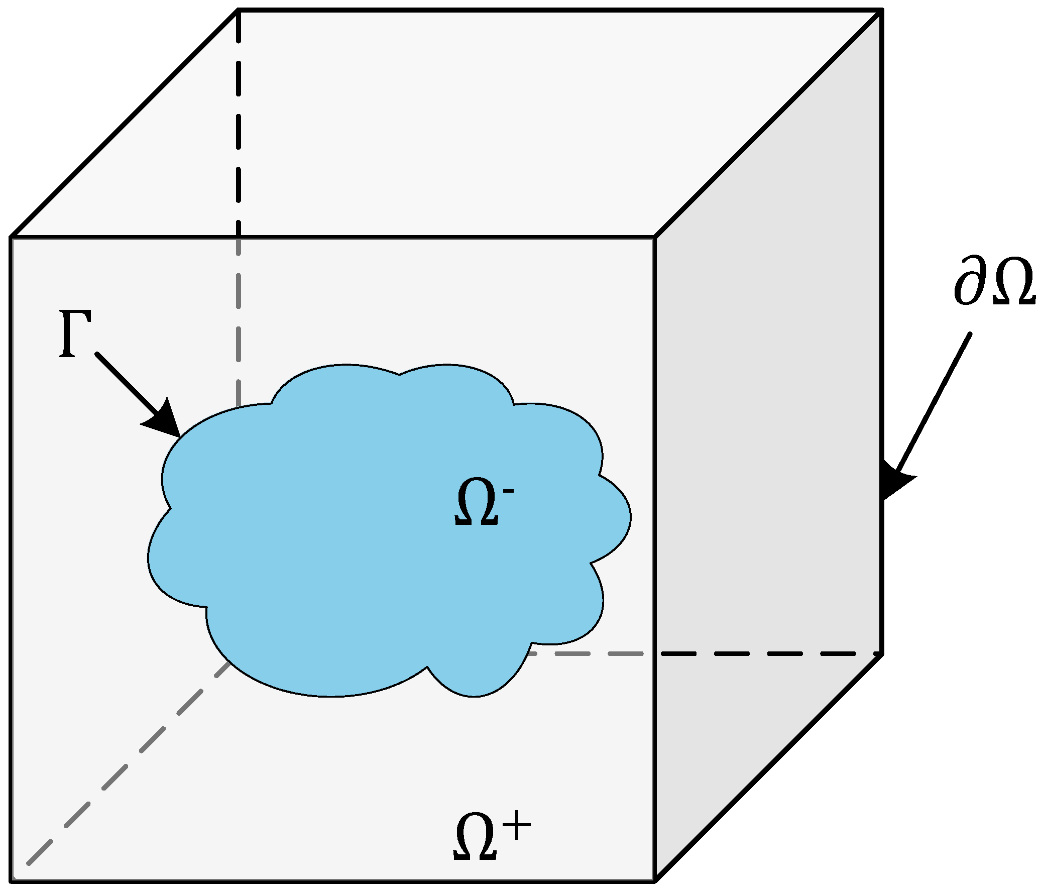
As shown in Figure 1, the model represents the problem of filling inhomogeneous anisotropic media. is the target region, a three-dimensional bounded open domain. is the interface of the medium that divides the target region into two subdomains, namely and . Naturally, the relationship between the target region and the subdomains can be expressed as . Assuming that the boundary of the target region and the boundary of each subdomain are Lipschitz continuous as submanifold, the interface of must also be Lipschitz continuous. Thus, unit normal vectors can be defined almost everywhere on interface , with the outer normal vector pointing from to .
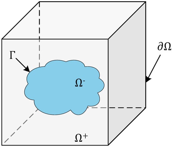
Figure 1.
Schematic diagram of the 3D interface problem model.
The Helmholtz equation accurately describes the nature of the acoustic field in inhomogeneous anisotropic media. Therefore, the Helmholtz equation governing the three-dimensional inhomogeneous anisotropic steady-state acoustic field is given by
where is the coordinates of points in the target region but not on interface of the medium, u denotes the sound field to be solved, ▽ denotes the gradient operator, is the wave number, and f is the source function. A parameter matrix is introduced into the equation to describe the acoustic wave propagation characteristics in different directions and spatial locations of the medium in the boundary value problem of the sound field. It is assumed that each component of the parameter matrix is continuously differentiable on the disjoint subdomains, but it may be discontinuous on interface . For the steady-state acoustic field in inhomogeneous media, the following representation is used to describe the medium in different subdomains,
The parameter matrix of the media are given in tensor form and expressed as follows:
where, the diagonal component of represents the propagation characteristics of sound waves propagating in each coordinate direction. The non-diagonal component represents the coupling effect between the various directions of the medium. If these components are imaginary, they represent the absorption effect when propagating in the non-coordinate axis direction.
2.2. Solution to the Three-Dimensional Inhomogeneous Anisotropic Steady-State Sound Field Problem
To reduce the regularity requirement of the solution, unify the expression form, simplify the treatment of boundary conditions, and enhance the stability and applicability of the numerical method, we use the variational method to derive the weak form of the integral equation, which is expressed as follows,
where , . is the Sobolev space,
b is a jump condition defined on interface . To address the above problems, we adopt a numerical method to solve the steady-state acoustic field in a three-dimensional irregular region filled with inhomogeneous anisotropic media, known as the Petrov–Galerkin finite element interface method (PGFEIM).
First, we introduce level set functions and to describe the cavity boundary and the medium interface . The level set function not only describes the geometry of the boundary but also helps distinguish the positional relationship between the grid points and the interface. The structure is as follows,
For the level set function , it describes the boundary of the target region. We can regard the boundary of the target region as a zero isosurface, and all the points on the boundary of the target region satisfy . For the points in the target region, the value of will be less than 0, and for the points outside the target region, the value of will be greater than 0. is a zero isosurface describing the medium interface in the target region. The value of is less than 0, indicating that the corresponding coordinate point is located in the internal medium; otherwise, it is located in the external medium.
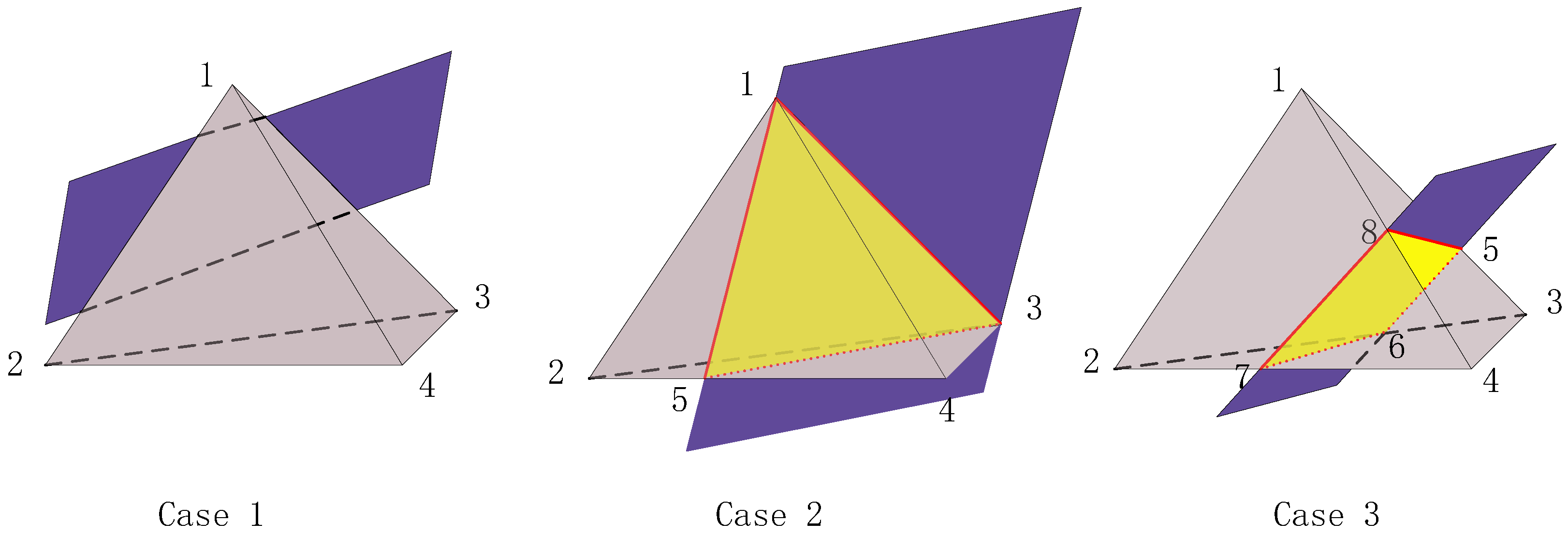
Secondly, to use a consistent Cartesian grid for unit subdivision, we restrict the target region to a regular virtual hexahedron and divide it into uniform cubes. To meet the requirements of the PGFEIM, each cube region must also be subdivided into six tetrahedral units, which serve as the final integration units. All the tetrahedral units obtained from the subdivision are collected into a set, denoted as . A unit L is said to be a regular unit if all its vertices lie within the same subdomain and the tetrahedral unit does not intersect any interface, as shown in Case 1 of Figure 2, where the gray tetrahedron represents unit L and the purple quadrilateral represents the interface or . Additionally, since the boundary of the target region or the interface dividing the internal media can have arbitrary shapes, the tetrahedral units may be truncated by these interfaces. If the vertices of a unit L lie on the interface or belong to different subdomains, the tetrahedral unit will intersect the interface, producing a yellow cross-section, as shown in Case 2 and Case 3 of Figure 2. Such a unit is called the interface unit. In the interface unit, we divide the unit into two parts, with the portions belonging to different subdomains labeled separately, denoted as . As shown in Case 3 of Figure 2, when a tetrahedral unit is truncated by a cross-section, the resulting decomposed part may contain non-tetrahedral shapes. In the PGFEIM, since the tetrahedral unit serves as the basic computational unit, any non-tetrahedral part must be further subdivided into tetrahedra. To minimize additional computational overhead, the number of newly generated tetrahedra should also be minimized.
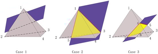
Figure 2.
Schematic diagram of the relationship between a tetrahedral unit and the interface.
In addition, there are two isomorphic mappings from the coefficient vectors to the finite element functions, denoted by and , respectively. For any test function , , it is a standard piecewise continuous linear function on a tetrahedral unit, and matches at the grid points. For any , is also a piecewise continuous linear function, and it matches at the grid points. In particular, in the regular unit, . In the interface unit, consists of two linear functions defined by and , respectively, and is discontinuous across , which is a cross-section within the tetrahedron.
Taking Case 3 as an example, we define that
The Dirichlet jump condition a along interface will be imposed at the vertex of the section . The Neumann jump condition b along interface is incorporated in its weak form and will be imposed at the centroid of the section . We divide section into two triangles, defining point 9 as the centroid of and point 10 as the centroid of . It is important to note that points 5, 6, 7, and 8 are not necessarily coplanar. We can obtain the following local linear system,
For each tetrahedral unit in , a set of partial linear systems can be derived. By solving these systems, the desired coefficient matrices are obtained. Then, by assembling the local matrices and solving the global system, a numerical solution to the problem is found. Thus, the original problem can always be transformed into solving the following equations,
3. U-Net Based Regression Network for Sliced Data
Three-dimensional physical fields play a crucial role in scientific research and engineering applications. However, reconstructing 3D problems is often hindered by the challenges of high-dimensional data storage and computational complexity. In this paper, we propose a method for the dimensionality reduction of the physical field through slicing. This approach enables efficient 3D reconstruction by decomposing the 3D physical field into 2D slices, offering significant advantages in capturing local properties and reducing computational complexity. The slicing method extracts 2D slices of the physical field along the X, Y, and Z axes, capturing local variations in each direction separately, thus enabling the accurate reconstruction of complex spatial distributions. Slice data are two-dimensional cross-sections obtained by fixing the value of one coordinate axis and recording the distribution of the physical field in the remaining two dimensions. As shown in Figure 3, the slicing method is shown. This approach significantly reduces the complexity of data processing by transforming the 3D physical field reconstruction problem into a combination of multiple 2D problems. By combining the deep learning model with the pixel-by-pixel regression method, we can efficiently reconstruct 3D physical fields. The slicing method offers high efficiency, flexibility, and a strong ability to capture local details.
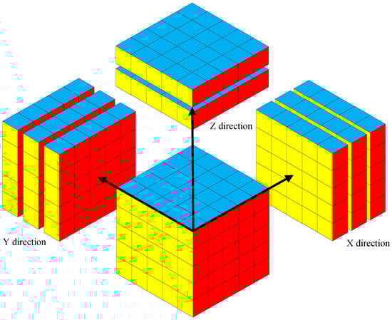
Figure 3.
Schematic diagram of the slicing method.
To perform pixel-by-pixel regression prediction for multi-directional sliced data, this paper designs a multi-channel regression network based on the U-Net architecture. The network efficiently reconstructs the parameter matrix of the 3D steady-state sound field by leveraging its strong feature extraction and spatial detail recovery capabilities from multi-channel data. The model adopts a symmetric U-shaped architecture, consisting of an encoder and a decoder. The encoder extracts high-level features through multilayer convolution and downsampling, while the decoder restores resolution through upsampling and uses skip connections to transfer low-level features directly from the encoder, enhancing detail expression while preserving global context information.
In the data processing section, data enhancement strategies are introduced to improve the model’s generalization and robustness. Specifically, random horizontal flipping helps the model learn symmetrical features and enhances its ability to recognize left–right flips. This helps the model to learn features from different perspectives,
where W is the image width. Random rotation further enhances the model’s ability to learn features of the physical field during training, increasing its invariance to rotational transformations. This renders the model independent of specific viewing angles, improving its adaptability to different input angles and reducing overfitting to specific training samples,
where is a random angle varying within the range of . By incorporating random translation, the model’s adaptability to images at different locations is enhanced. This allows the model to correctly predict even the time the location of the physical field changes, avoiding reliance on a specific location,
where , . These enhancement strategies can not only improve the robustness of the model on different input data, but they can also effectively deal with some challenges in sound field reconstruction. For example, random flipping and rotation can help the model learn symmetric features, rather than relying solely on fixed directions. Random translation is used to simulate the spatial change of data, which helps the model to perceive the change of location and avoid relying on a specific location. The proposed enhancement strategy can effectively avoid the inversion error caused by the position offset during the sound field data acquisition process, thereby improving the generalization ability and robustness of the model in practical application scenarios.
The input to the network is multi-channel slice data of size , containing slices in the X, Y, and Z directions, with each direction providing two sets of slice features representing different physical attributes. The output dimension of the model is the same as the input, also , where each channel represents the regression prediction result for the corresponding pixel.
The encoder part of the network consists of a three-layer convolutional module. Each convolutional module contains a convolutional layer to extract local features, with ReLU as the activation function to introduce nonlinearity. Batch normalization is applied after each convolutional layer to accelerate training convergence and improve model stability. After each convolutional layer, the feature maps are downsampled using a max-pooling operation, gradually reducing the spatial resolution while extracting higher-level semantic features.
In the decoder section, the model uses an inverse convolution operation for upsampling to recover the resolution lost during downsampling. At the same time, skip connections are used in each decoding module to combine the features from the encoder with those at the corresponding resolution in the decoder. The introduction of skip connections allows the decoder to combine low-level features from the encoder with high-level semantic features, preserving spatial details while enhancing contextual information. This feature fusion mechanism is particularly effective for pixel-by-pixel regression tasks. Each decoding module also includes a convolutional layer, ReLU activation function, and batch normalization to ensure effective feature extraction and network robustness. Finally, the output of the decoder is mapped onto six channels in the model’s output layer by a convolutional layer, with each channel corresponding to a specific physical attribute.
To accommodate the pixel-by-pixel regression task, the output layer uses a regression loss function to optimize the gap between the network’s predictions and the true labels. The regression loss function here uses the mean square error,
Among them, is the predicted value of the network, is the real label, and N is the number of samples. By optimizing this loss function, the network gradually approaches the real physical field distribution, thereby achieving efficient reconstruction.
In the model training phase, the Adam optimizer was used with an initial learning rate of 0.1. To further optimize the training process and avoid becoming stuck in local optima, a dynamic learning rate adjustment strategy is introduced in this paper,
where is the initial learning rate, is the rate at which the learning rate decreases at each step, k is the period at which the learning rate is reduced, and t is the current epoch. The strategy used in this paper is to reduce the learning rate to 10% of the original rate after every 30 training epochs. During the training process, the dataset is randomly split into a training set, a validation set, and a test set. The training set is used to update the network weights, the validation set is used to monitor the model’s performance in real time, and the test set is used for final performance evaluation. By adopting a symmetric U-shaped architecture, multi-channel feature input processing, and a skip connection mechanism, the model designed in this paper can extract global semantic information while preserving rich spatial details, resulting in highly accurate and spatially consistent pixel-by-pixel predictions. This model offers an efficient and robust solution to the problem of physical field reconstruction in complex regression tasks.
4. Numerical Examples and Results
In this section, a series of numerical experiments demonstrate the feasibility and efficiency of the U-Net based regression network for sliced data. We analyze the results in detail using evaluation metrics such as the Mean Squared Error (MSE), Normalized Mean Squared Error (NMSE), Peak Signal-to-Noise Ratio (PSNR), and Structural Similarity Index (SSIM),
Among the four metrics, MSE measures the average squared difference between the predicted and true values, reflecting the magnitude of the prediction error. NMSE is a normalization of MSE, which scales the error relative to the true value, making it more suitable for comparing data across different scales or domains. The closer the NMSE value is to 0, the more accurate the prediction. PSNR is used to evaluate the similarity between the predicted and the actual images. The higher the PSNR value, the smaller the difference between the two images, indicating higher quality. The SSIM evaluates the perceived quality of an image in terms of brightness, contrast, and structure, which aligns more closely with human visual perception. The closer the SSIM value is to 1, the more similar the two images are. In the task of sound field reconstruction, MSE and NMSE constitute quantitative evaluation criteria to measure the numerical accuracy of physical quantity inversion results. At the same time, PSNR and SSIM are introduced to construct a visual evaluation dimension in order to display the inverted sound field more intuitively.
4.1. Example 1
In this example, we assume a cubic region Ω with a size of 1 m3, containing a sphere of radius 0.4 m embedded inside, as shown in the Figure 4. The goal of the experiment is to reconstruct the size and distribution of the parameter matrix in the target region, in order to obtain the shape of the internal medium.

Figure 4.
Steady-state sound field problem of the regular region with spherical interface.
Specifically, the parameter matrix for the target region is given as follows,
The parameters on the outside of the sphere remain unchanged. The parameters inside the sphere vary in the Z direction, with the real part a ranging from 1 to 1.95 in steps of 0.05, and the imaginary part b ranging from 4 to 4.95 in steps of 0.05. This resulted in a 400-group of parameter matrices with different values, and the corresponding sound field data were obtained using the PGFEIM. The data were then sliced in the X, Y, and Z directions, with each direction divided into 32 parts. After removing the invalid slices that do not contain useful information, 10,000 valid data in different directions are obtained, each with a size of . Each piece of data also contains information about the real and imaginary parts. The real and imaginary parts of each data are then separated to create a dataset of size . We randomly select 80% of the data as the training set, 10% as the validation set, and 10% as the test set.
As shown in Figure 5, from left to right and from top to bottom, the two images are a group. The left side is the real image, and the right side is the prediction result, which shows one inversion result in each channel in turn. From the figure, it can be observed that the U-Net based regression model for sliced data successfully predicts the medium interface in the real sliced image. The predicted results closely resemble the actual structure, particularly in terms of interface localization, where the demarcation positions of the predicted and real images almost completely overlap, indicating the high accuracy of the model.
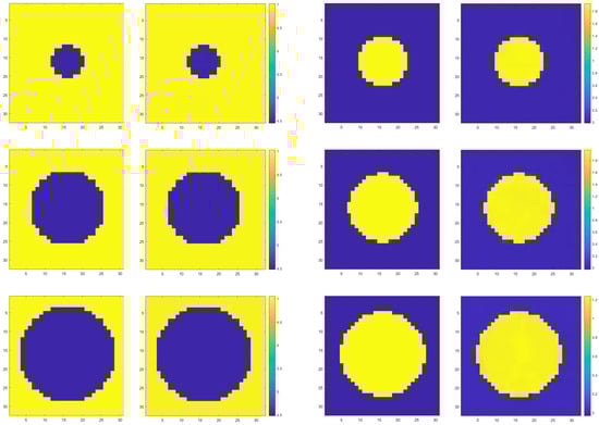
Figure 5.
Demonstration of inversion results of spherical interface in different channels.
In order to provide a more objective evaluation, we conducted a quantitative analysis of the experimental results. Specifically, we used the commonly employed evaluation metrics, including mean squared error, peak signal-to-noise ratio, and structural similarity index. Each evaluation metric assesses image quality from different aspects. For example, MSE and PSNR mainly evaluate pixel-level differences, while SSIM focuses on perceived quality, structure, contrast, and similarity between the predicted and real images. As the data in Table 1 show, MSE is very small, indicating that the predicted results are very close to the real value. The SSIM also shows that the similarity between images is very large in numerical terms. The PSNR values are between 30 and 50, indicating that the quality of the prediction results are high. The evaluation metrics indicate that the reconstruction results are highly accurate in localized areas, demonstrating the model’s strong capability to capture details.

Table 1.
Evaluation metrics for the example in Figure 5.
Since the target region is a cube, its boundary has no reference value in this example, so the reconstruction of this example focuses on the interface of the internal media. Figure 6 shows a slice view of the inversion results. It can be seen from the figure that the reconstructed medium interface is very clear. Table 2 lists the evaluation metrics of the inversion results of the test samples in different channels. Both MSE and NMSE remain at a low level, indicating that the error of the reconstruction results is very small and the quality is excellent. The SSIM results indicate that the model achieves an excellent reconstruction effect on different channels, with the reconstructed image preserving structural information and ensuring high visual fidelity. Therefore, this model not only accurately restores the interface of the media in the target region, but it also reconstructs the parameter matrix of the target region and achieves high accuracy. Numerical experiments show that the model has a good reconstruction ability for the sound field of a three-dimensional regular region filled with media.

Figure 6.
Slice diagram of inversion results for homogeneous anisotropic media.
Table 2.
Evaluation metrics for inversion results of homogeneous anisotropic media in different channels.
4.2. Example 2
In order to verify that our method can not only accurately capture the interface of the media but also reconstruct the target region with irregular shape, we conduct further experiments. We set the target region as a sphere with a radius of 0.5 m, with a four-pointed star embedded inside, as shown in Figure 7.

Figure 7.
Steady-state sound field problem of the irregular region with inhomogeneous media interface.
To be specific, we define the parameter matrix of the medium in the target region as follows,
denotes the medium surrounding the four-pointed star, and its value remains constant. denotes the medium inside the four-pointed star. In the Z direction, the real part a varies from 4 to 4.95 in steps of 0.05, and the imaginary part b varies from 1 to 1.95 in increments of 0.05. This results in a 400-group parameter matrix, and the sound field data were obtained using the PGFEIM. Similarly, these data are sliced along the X, Y, and Z directions, with each direction divided into 32 parts, resulting in 12,800 sliced data. We randomly select 80% of the data as the training set, 10% as the validation set, and 10% as the test set.
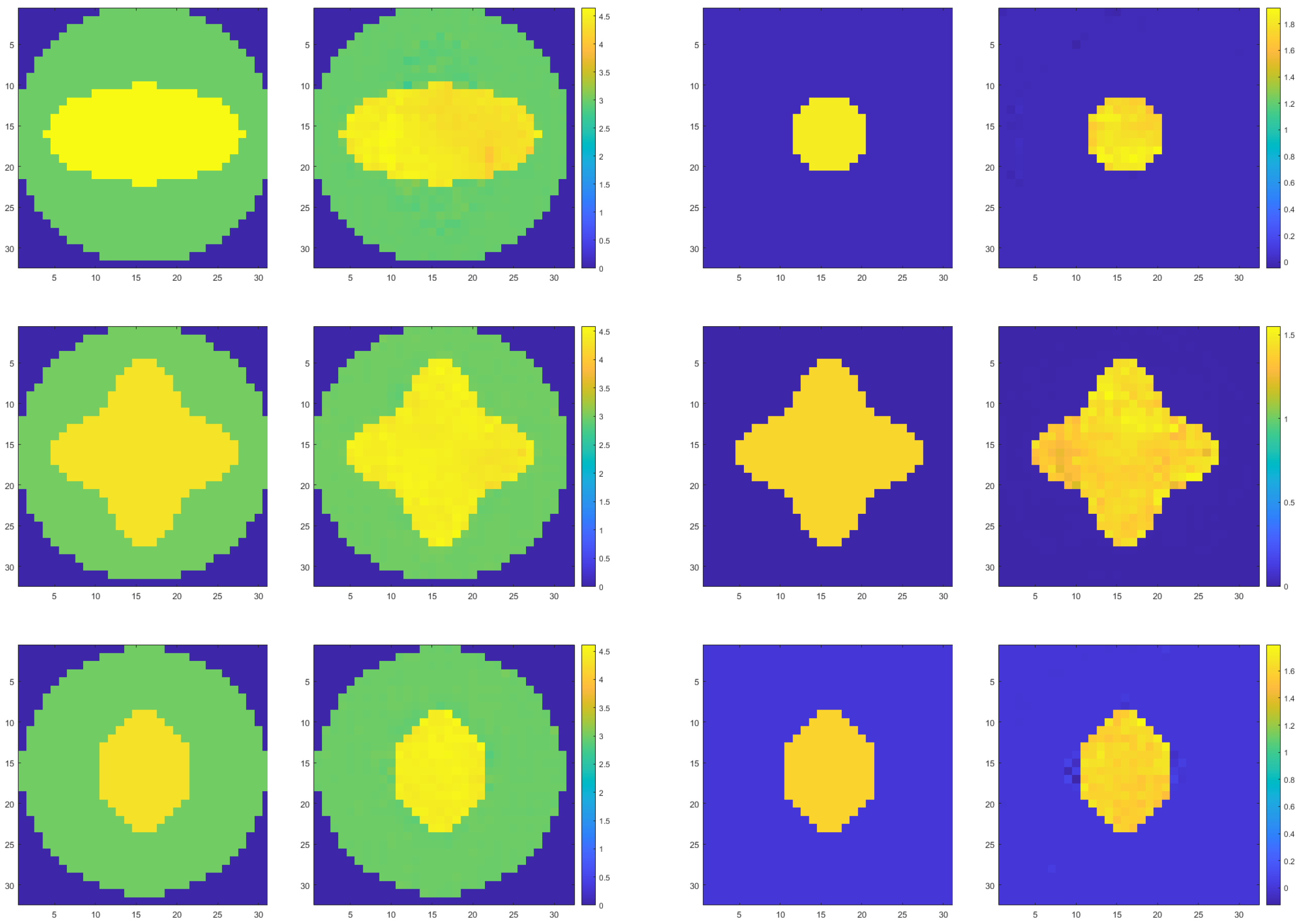
As shown in Figure 8, from left to right and from top to bottom, the two images are a group. The left side is the real image, and the right side is the prediction result, which shows one inversion result in each channel in turn. From the figure, it is found that that the reconstruction effect of the internal medium is suboptimal in terms of visual quality, but the model still accurately identifies the boundary of the target region and captures the irregular medium interface. Table 3 lists the PSNR, MSE, and SSIM of the six sets of experimental results in Figure 8. MSE is still very small, indicating that the predicted results are very close to the real value. The value of SSIM also shows that the similarity between images is very large. Although the PSNR values are lower than those of Example 1, they still remain at a high level, indicating that the quality of the prediction results remains high. The evaluation metrics numerically indicate that the reconstruction results are excellent. By examining the imaging data, it is observed that the numerical value of the reconstructed internal medium is very close to the true value, though the imaging quality is slightly inferior.
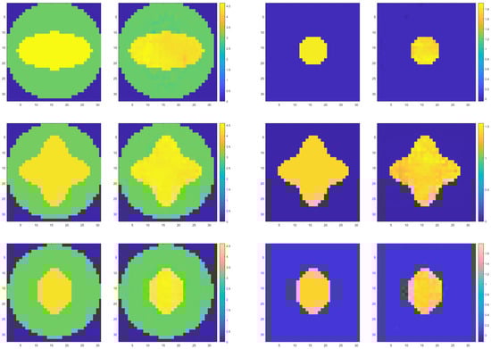
Figure 8.
Demonstration of inversion results of inhomogeneous media interface in different channels.
Table 3.
Evaluation metrics for the example in Figure 8.
Figure 9 shows a slice view of the inversion results. The boundary of the target region, the interface of the internal media, and the geometry of the internal region are clearly visible in the figure. Table 4 lists the evaluation metrics of the inversion results of the test samples in different channels. The MSE and NMSE remain at low levels, and the SSIM results show that the reconstruction quality across different channels remains high. This example effectively verifies that the model can well reconstruct different interfaces and parameter matrices in the target region even in the face of inhomogeneous anisotropic irregular target region.

Figure 9.
Slice diagram of the inversion results for inhomogeneous anisotropic media.
Table 4.
Evaluation metrics for the inversion results of inhomogeneous anisotropic media in different channels.
4.3. Example 3
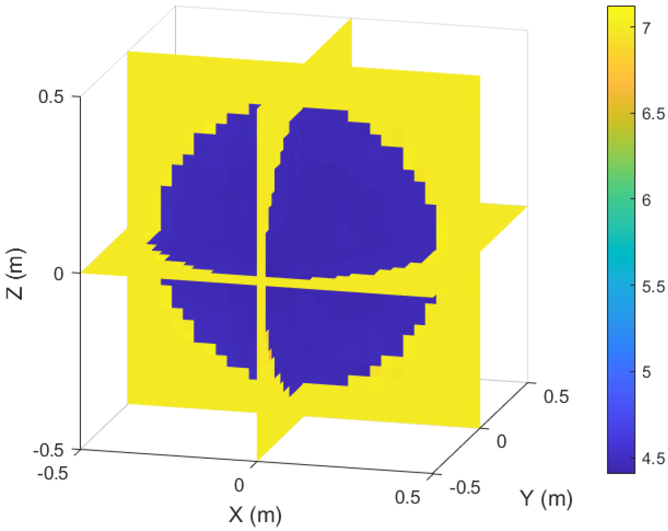
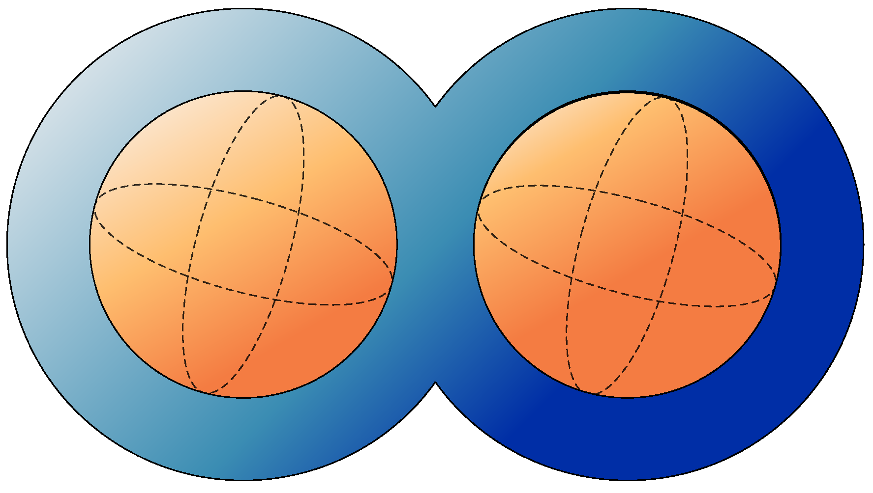
To further verify the strong reconstruction capability of our method for the irregular target region, we define a non-convex target region with two spherical internal media interface in this example, which is represented by the following level set function,
From the level set functions, it can be seen that the target region is formed by the concatenation of two spheres with a radius of 0.25 m, centered at and . Inside these, there are two independent spheres with a radius of 0.15 m, centered at and .
Figure 10 presents the geometry of the target region described by the level set function. The parameter matrix of the filling media in the target region is represented as follows,
denotes the medium parameter that fills the target region, excluding the two independent spheres, with a constant value. denotes the medium parameter filled in the internally independent spheres. In the Z direction, the real part a varies from 5 to 5.95 in steps of 0.05, and the imaginary part b varies from 3 to 3.95 in increments of 0.05. This results in a 400-group parameter matrix, and the sound field data were obtained using the PGFEIM. Similarly, these data are sliced along the X, Y, and Z directions, with each direction divided into 32 parts, resulting in 12,800 sliced data. We randomly select 80% of the data as the training set, 10% as the validation set, and 10% as the test set.
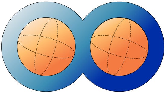
Figure 10.
Steady-state sound field problem of the irregular non-convex region with spherical media interface.
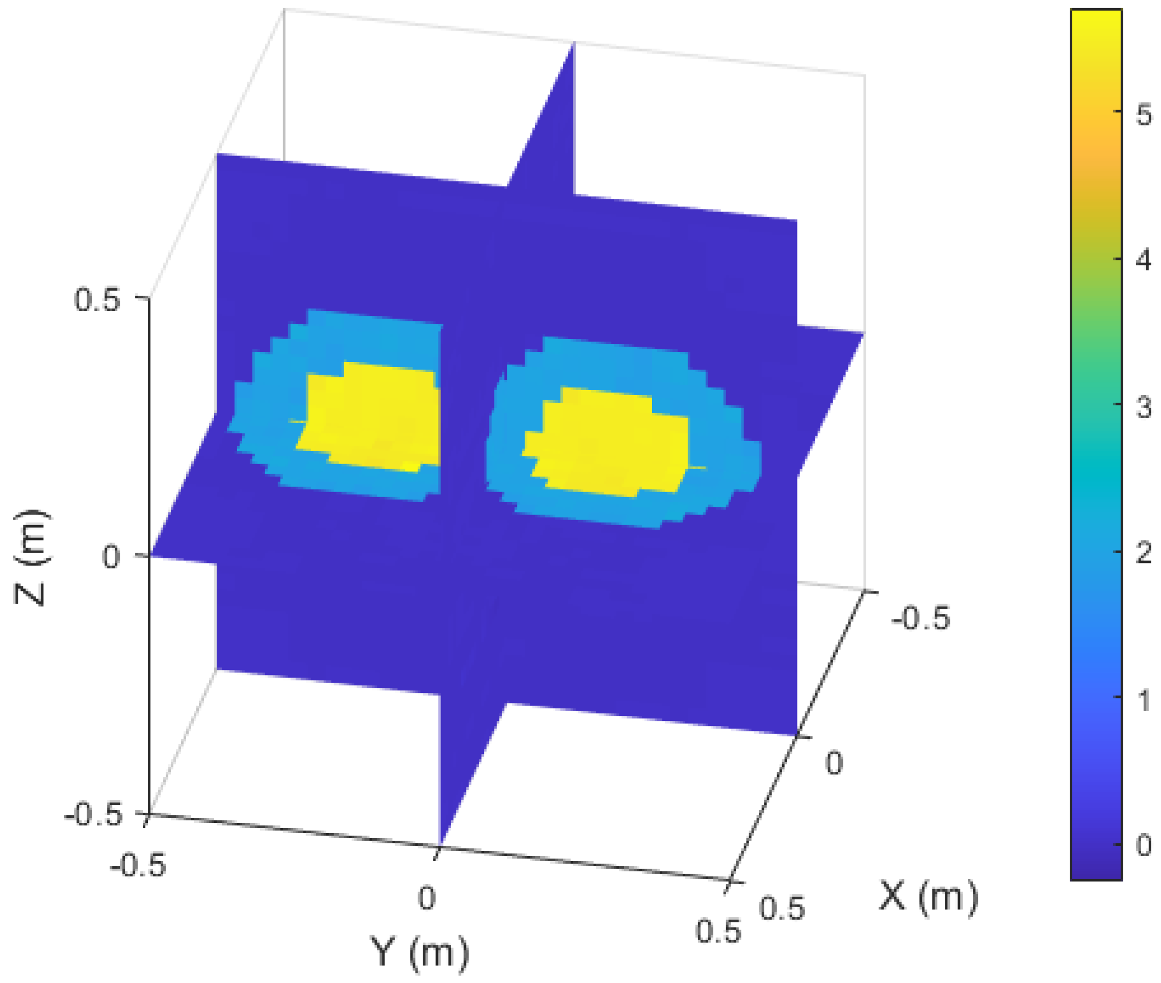
As shown in Figure 11, from left to right and from top to bottom, the two images are a group. The left side is the real image, and the right side is the prediction result, which shows one inversion result in each channel in turn. By observing the local slice diagrams, it can be seen that the model successfully reconstructs the non-convex region, with the diagrams clearly showing the boundary of the target region as well as the interfaces of filling media. Table 5 lists the PSNR, MSE, and SSIM of the six sets of experimental results in Figure 11. The data in the table show that, even for the non-convex region, the model’s reconstruction in localized areas is excellent, further verifying its strong ability to capture details.
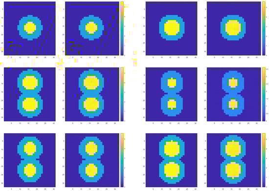
Figure 11.
Demonstration of inversion results of inhomogeneous media interfaces in different channels.
Table 5.
Evaluation metrics for the example in Figure 11.
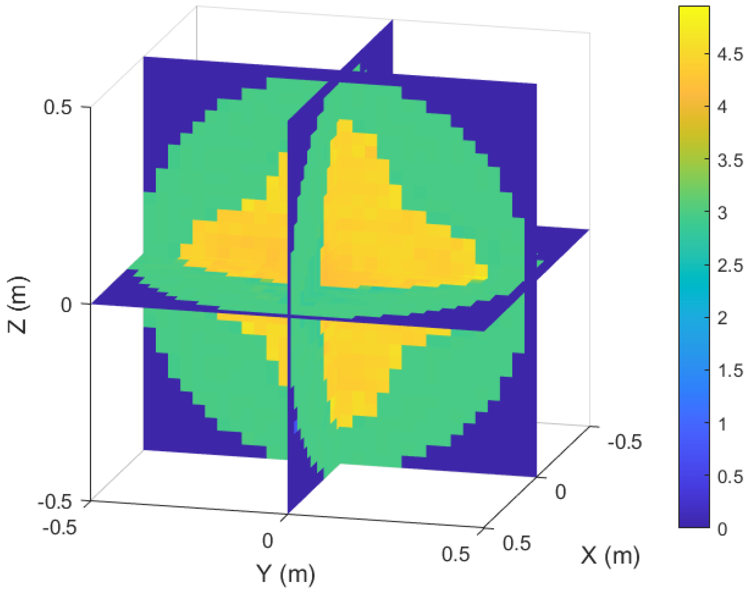
Figure 12 shows a slice view of the inversion results. Even if the target region is non-convex and there are independent media inside, the boundary of the non-convex target region, the interfaces of the internal media and the geometry of the internal areas can still be clearly observed in the figure. Table 6 lists the evaluation metrics of the inversion results of the test samples in different channels. The MSE and NMSE remain low, and the SSIM results show that the model still achieves excellent reconstruction, even for irregular non-convex region. This example further validates that the model can not only accurately restore the complex structure of the target region, but it can also reconstruct the media in different regions.

Figure 12.
Slice diagram of the inversion results of the irregular non-convex region with a spherical media interface.
Table 6.
Evaluation metrics for inversion results of inhomogeneous anisotropic media in different channels.
5. Conclusions
The PGFEIM used in this paper effectively generates the initial data for different scenarios. By introducing the slicing method, the 3D problem is successfully decomposed into a combination of 2D problems, reducing computational cost. We propose a U-Net based regression network model for sliced data to reconstruct a three-dimensional irregular sound field filling inhomogeneous anisotropic media. We use three examples to verify that the model can accurately capture various interfaces in the target region, such as the boundary of the target region and the interface of the media. Even when the media are distributed in different regions, the model can effectively capture its boundaries. In the face of complex structures, such as a non-convex region, the model can also effectively reconstruct its geometric structure and medium distribution. In addition, the model also reconstructs the parameter matrix describing the medium in the target region, successfully achieving accurate sound field reconstruction. The method successfully realizes the dual reconstruction of the shape and parameters of the three-dimensional steady-state sound field, and provides a solution to the sound field inversion problem. Although the method performs well in the above aspects, it also has some limitations. The scope of application of the method is not wide enough. The current work mainly focuses on the application of static equations, and has not yet involved dynamic problems. Based on the limitations of the current method, we will consider expanding on these two aspects in the future. By optimizing the U-Net network model, we improve its handling of more complex media changes. The method is extended to the dynamic sound field problem, and ways to deal with the problem of time dependence have been discussed.
Author Contributions
Conceptualization, Z.S.; methodology, Z.S.; writing—original draft preparation, Z.S.; project administration, W.Z.; supervision, W.Z.; writing—review and editing, M.Z. All authors have read and agreed to the published version of the manuscript.
Funding
This research was funded by the Natural Science Foundation of Hebei Province (No. A2024502009) and the Fundamental Research Funds for the Central Universities (No. 2021MS115).
Data Availability Statement
The original contributions to this study can be found in the article. For further inquiries, please contact the corresponding author.
Acknowledgments
The authors would like to thank the referees for their very helpful comments.
Conflicts of Interest
The authors declare no conflicts of interest.
References
- Sarvazyan, A.P.; Urban, M.W.; Greenleaf, J.F. Acoustic waves in medical imaging and diagnostics. Ultrasound Med. Biol. 2013, 39, 1133–1146. [Google Scholar] [CrossRef] [PubMed]
- Nadimi, N.; Javidan, R.; Layeghi, K. Efficient detection of underwater natural gas pipeline leak based on synthetic aperture sonar (SAS) systems. J. Mar. Sci. Eng. 2021, 9, 1273. [Google Scholar] [CrossRef]
- Cosarinsky, G.; Fernandez-Cruza, J.; Camacho, J. Plane wave imaging through interfaces. Sensors 2021, 21, 4967. [Google Scholar] [CrossRef]
- Li, F.; Villa, U.; Duric, N.; Anastasio, M.A. 3D full-waveform inversion in ultrasound computed tomography employing a ring-array. In Medical Imaging 2023: Ultrasonic Imaging and Tomography; SPIE: Bellingham, WC, USA, 2023; Volume 12470, pp. 99–104. [Google Scholar]
- Dommergues, B.; Cruz, E.; Vaz, G. Optimization of underwater acoustic detection of marine mammals and ships using CNN. In Proceedings of Meetings on Acoustics; AIP Publishing: Melville, NY, USA, 2022; Volume 47, p. 1. [Google Scholar]
- Pierri, R.; Leone, G. Inverse scattering of dielectric cylinders by a second-order Born approximation. IEEE Trans. Geosci. Remote Sens. 1999, 37, 374–382. [Google Scholar]
- Gao, G.; Torres-Verdin, C. High-order generalized extended Born approximation for electromagnetic scattering. IEEE Trans. Antennas Propag. 2006, 54, 1243–1256. [Google Scholar]
- Dubey, A.; Chen, X.; Murch, R. A new correction to the Rytov approximation for strongly scattering lossy media. IEEE Trans. Antennas Propag. 2022, 70, 10851–10864. [Google Scholar]
- Yin, T.; Pan, L.; Chen, X. Subspace-Rytov approximation inversion method for inverse scattering problems. IEEE Trans. Antennas Propag. 2022, 70, 10925–10935. [Google Scholar] [CrossRef]
- Yin, T.; Pan, L.; Chen, X. Subspace-based distorted-Rytov iterative method for solving inverse scattering problems. IEEE Trans. Antennas Propag. 2023, 71, 8173–8183. [Google Scholar]
- De Zaeytijd, J.; Franchois, A.; Eyraud, C.; Geffrin, J.-M. Full-wave three-dimensional microwave imaging with a regularized Gauss–Newton method—Theory and experiment. IEEE Trans. Antennas Propag. 2007, 55, 3279–3292. [Google Scholar]
- Üregen, E.; Yapar, A. Focusing-Based Newton Solution for Electromagnetic Inverse Scattering Problems. IEEE Trans. Antennas Propag. 2024; in press. [Google Scholar]
- Mojabi, P.; LoVetri, J. Comparison of TE and TM inversions in the framework of the Gauss–Newton method. IEEE Trans. Antennas Propag. 2010, 58, 1336–1348. [Google Scholar] [CrossRef]
- Yaswanth, K.; Bhattacharya, S.; Khankhoje, U.K. Algebraic reconstruction techniques for inverse imaging. In Proceedings of the 2016 International Conference on Electromagnetics in Advanced Applications (ICEAA), Cairns, QLD, Australia, 19–23 September 2016; pp. 756–759. [Google Scholar]
- Bagci, H.; Raich, R.; Hero, A.E.; Michielssen, E. Sparsity-regularized Born iterations for electromagnetic inverse scattering. In Proceedings of the 2008 IEEE Antennas and Propagation Society International Symposium, San Diego, CA, USA, 5–11 July 2008; pp. 1–4. [Google Scholar]
- Lechleiter, A.; Rennoch, M. Non-linear Tikhonov regularization in Banach spaces for inverse scattering from anisotropic penetrable media. Inverse Probl. Imaging 2017, 11, 151–176. [Google Scholar] [CrossRef]
- Kamilov, U.S.; Liu, D.; Mansour, H.; Boufounos, P.T. A recursive Born approach to nonlinear inverse scattering. IEEE Signal Process. Lett. 2016, 23, 1052–1056. [Google Scholar] [CrossRef]
- Li, L.; Wang, L.G.; Teixeira, F.L. Performance analysis and dynamic evolution of deep convolutional neural network for electromagnetic inverse scattering. IEEE Antennas Wirel. Propag. Lett. 2019, 18, 2259–2263. [Google Scholar] [CrossRef]
- Wei, Z.; Chen, X. Physics-inspired convolutional neural network for solving full-wave inverse scattering problems. IEEE Trans. Antennas Propag. 2019, 67, 6138–6148. [Google Scholar] [CrossRef]
- Xiao, J.; Li, J.; Chen, Y.; Han, F.; Liu, Q.H. Fast electromagnetic inversion of inhomogeneous scatterers embedded in layered media by Born approximation and 3-D U-Net. IEEE Geosci. Remote Sens. Lett. 2019, 17, 1677–1681. [Google Scholar] [CrossRef]
- Li, H.; Chen, L.; Qiu, J. Convolutional neural networks for multifrequency electromagnetic inverse problems. IEEE Antennas Wirel. Propag. Lett. 2021, 20, 1424–1428. [Google Scholar] [CrossRef]
- Xu, K.; Zhang, C.; Ye, X.; Song, R. Fast full-wave electromagnetic inverse scattering based on scalable cascaded convolutional neural networks. IEEE Trans. Geosci. Remote Sens. 2021, 60, 2001611. [Google Scholar] [CrossRef]
- Aydın, İ.; Budak, G.; Sefer, A.; Yapar, A. CNN-based deep learning architecture for electromagnetic imaging of rough surface profiles. IEEE Trans. Antennas Propag. 2022, 70, 9752–9763. [Google Scholar] [CrossRef]
- Zhang, Y.; Lambert, M.; Fraysse, A.; Lesselier, D. Unrolled convolutional neural network for full-wave inverse scattering. IEEE Trans. Antennas Propag. 2022, 71, 947–956. [Google Scholar] [CrossRef]
- Barmada, S.; Di Barba, P.; Fontana, N.; Mognaschi, M.E.; Tucci, M. Electromagnetic field reconstruction and source identification using conditional variational autoencoder and CNN. IEEE J. Multiscale Multiphysics Comput. Tech. 2023, 8, 322–331. [Google Scholar] [CrossRef]
- Puzyrev, V. Deep learning electromagnetic inversion with convolutional neural networks. Geophys. J. Int. 2019, 218, 817–832. [Google Scholar] [CrossRef]
- Yao, H.M.; Jiang, L.; Wei, E.I. Enhanced deep learning approach based on the deep convolutional encoder–decoder architecture for electromagnetic inverse scattering problems. IEEE Antennas Wirel. Propag. Lett. 2020, 19, 1211–1215. [Google Scholar] [CrossRef]
- Ye, X.; Bai, Y.; Song, R.; Xu, K.; An, J. An inhomogeneous background imaging method based on generative adversarial network. IEEE Trans. Microw. Theory Tech. 2020, 68, 4684–4693. [Google Scholar] [CrossRef]
- Song, R.; Huang, Y.; Xu, K.; Ye, X.; Li, C.; Chen, X. Electromagnetic inverse scattering with perceptual generative adversarial networks. IEEE Trans. Comput. Imaging 2021, 7, 689–699. [Google Scholar] [CrossRef]
- Hu, Y.D.; Wang, X.H.; Zhou, H.; Wang, L.; Wang, B.Z. A more general electromagnetic inverse scattering method based on physics-informed neural network. IEEE Trans. Geosci. Remote Sens. 2023, 61, 4505109. [Google Scholar] [CrossRef]


Disclaimer/Publisher’s Note: The statements, opinions and data contained in all publications are solely those of the individual author(s) and contributor(s) and not of MDPI and/or the editor(s). MDPI and/or the editor(s) disclaim responsibility for any injury to people or property resulting from any ideas, methods, instructions or products referred to in the content. |
© 2025 by the authors. Licensee MDPI, Basel, Switzerland. This article is an open access article distributed under the terms and conditions of the Creative Commons Attribution (CC BY) license (https://creativecommons.org/licenses/by/4.0/).