Equilibrium Points and Periodic Orbits in the Circular Restricted Synchronous Three-Body Problem with Radiation and Mass Dipole Effects: Application to Asteroid 2001SN₂₆₃

Abstract

This study numerically explores the dynamics of the photogravitational circular restricted three-body problem, where an infinitesimal particle moves under the gravitational influence of two primary bodies connected by a massless rod. These primary masses revolve in circular orbits around their common center of mass, which remains fixed at the origin of the coordinate system. The distance between the two masses remains constant, independent of their rotation period. The third body, being infinitesimally small compared to the primary masses, has a negligible effect on their motion. The primary mass is considered as a radiating body, while the secondary is modeled as an elongated one comprising two hypothetical point masses separated by a fixed distance. The analysis focuses on determining the number, location, and stability of equilibrium points, as well as examining the structure of zero-velocity curves under the influence of system parameters such as mass and force ratio, radiation pressure and geometric configuration of the secondary body. The system is found to allow up to six equilibria: four collinear and two non-collinear. Their number and positions are significantly affected by variations in the system’s parameters. Stability analysis reveals that the two non-collinear equilibrium points can exhibit stability under specific parameter configurations, while the four collinear points are typically unstable. An exception is the innermost collinear equilibrium point, which can be stable for certain parameter values. Our numerical investigation on periodic orbits around the collinear equilibrium points of the asteroid triple-system 2001SN₂₆₃ show that a variation, either to the values of radiation or the force ratio parameters, influence their special characteristics such as period and stability. Also, their continuation in the space of initial conditions shows that all families terminate naturally at collision orbits with either the primary or the secondary.

1. Introduction

The Circular Restricted Three-Body Problem (CRTBP) examines the motion of a negligible mass moving within a system of two massive bodies, referred to as the primaries, which orbit each other around their common center of mass. The third body (test particle) is much smaller in mass than the primaries, so its influence on their motion is negligible. As the CRTBP is a non-integrable dynamical system, analytical solutions for the particle’s orbit are generally not obtainable [1], requiring the use of numerical methods for deeper analysis. In the context of the planar gravitational restricted three-body problem, there are five equilibrium points. Among these, the equilateral points $L_4$ and $L_5$ are stable when the mass ratio $\mu$ of the primaries is below the critical threshold ${\mu }_0\cong 0.03852090.$ In contrast, the other three collinear points $L_1$, $L_2$ and $L_3$ are typically unstable.

To understand and analyze the dynamical behavior of a test particle in the CRTBP, numerous researchers have extended this classical problem by introducing additional factors. These generalized restricted three-body problems incorporate extra hypotheses that modify the original CRTBP but without changing its basic nature. Such extensions may include the effects of radiation pressure, Poynting–Robertson drag, and the Yarkovsky effect, among others. While the Yarkovsky effect may have a relatively small influence, it is particularly important in celestial mechanics, especially when determining the proper orbits of small celestial bodies, like asteroids. Among all these perturbative forces, radiation pressure stands out as the most significant. The interest in the dynamics of small particles within solar systems containing one or two stars has led to the development of the so-called Photogravitational Restricted Three-Body Problem (PRTBP). This model is particularly useful for investigating the dynamics within such systems. Radzievskii is credited with being the first to consider this problem, discussing it in the context of three bodies: the Sun, a planet, and a dust particle [2]. His work showed that accounting for direct solar electromagnetic radiation alters the positions of the equilibrium points. Since then, many researchers have explored the effects of radiation pressure on the dynamics of these systems (see [3,4,5,6,7,8,9], among others). Another key area of research in the PRTBP involves the computation of families of periodic orbits [10,11,12,13]. Additionally, there are various extensions of the three-body problem that include more than two finite bodies. For example, when a planetary system consists of three primary bodies (such as one, two, or three stars) and a small mass, it leads to the Photogravitational Restricted Four-Body Problem. This is an area of ongoing study with several contributions (see, for example, [14,15,16,17,18,19]). These models are highly relevant because they more accurately reflect the dynamics of real-world systems. The studies mentioned above are instrumental for understanding the modified dipole problem discussed in this paper, and their findings will certainly aid in its analysis.

Asteroids, unlike planets, are small celestial bodies with irregular shapes and feeble gravitational fields. These distinct characteristics make the study of the forces affecting objects near asteroids critical for space missions targeting these bodies. Recent research has rekindled interest in understanding the dynamics of particles in the vicinity of asteroids, particularly those with elongated or irregular forms. In [20], the equilibrium points of twenty-three minor celestial bodies were explored, such as asteroids, comets, and planet moonlets by utilizing advanced radar data to model their gravitational fields. Their work highlighted how the distribution, location, and stability of equilibrium points are strongly influenced by the shape, mass distribution, and rotational period of the bodies in question. In a similar line of inquiry, in [21], a perturbed version of the restricted three-body problem was examined, focusing on a system where the smaller primary has an elongated shape and the larger one is oblate, and emits radiation. In [22], a model of two elongated bodies linked by a massless rod (the dipole configuration) was addressed, paying particular attention to the stability of equilibrium points when gravitational forces outweigh centrifugal forces. Their work was later extended by the authors of [23], who provided further insights into the specific conditions under which stability could be achieved. Particularly, in [22], it was shown that external collinear equilibrium points $L_{2,3}$ are linearly unstable, while in [23] it was demonstrated that the inner equilibrium point $L_1$ exhibits conditional stability in some cases, adding thus another layer of complexity to the dynamical behavior of this problem. Furthermore, triangular equilibrium points $L_{4,5}$ were found to be conditionally stable.

Furthermore, in [24], the dynamics of a rotating dipole mass system was investigated, a model that can describe synchronous asteroid systems. That work introduced several modifications to the traditional dipole model with follow-up studies, exploring various perturbative effects on the system [25,26]. Recently, new perturbed versions of the CRTBP that consider the effects of quantum corrections have been introduced [27]. Based on that work, in [28], this model was simplified by effectively creating the quantized Hill problem. These new models represent a step toward a quantized version of the restricted three-body problem, opening up new avenues for the study of small celestial bodies under the influence of both classical and quantum effects.

The Circular Restricted Synchronous Three-Body Problem (CRSTBP) represents an extension of the classical dipole model by incorporating a more complex set of dynamical equations. This problem examines the motion of a negligible mass within a system consisting of two massive bodies in circular orbits around their common center of mass. In this system, one body is modeled as spherical while the other is represented by a synchronous rotating dipole formed by two hypothetical bodies of equal mass separated by a fixed distance. Building on the foundational work of the classical dipole model, in [29,30], the CRSTBP was analyzed, investigating the periodic orbits, accessible regions of motion, positions and stability of equilibrium points. Drawing inspiration from [29], in [31], this analysis was extended by examining the equilibrium points and their linear stability within the elliptic restricted synchronous three-body problem that includes a mass dipole. Additionally, within the same framework, in [32] the effects of oblateness in the larger primary body were explored, focusing on the stability and velocity sensitivities of the libration points in the elliptic restricted three-body context. Recently, in [33], the equilibrium points and Lyapunov families were investigated, incorporating an oblate parameter in the CRTBP with a rotating mass dipole. Their work further refines the understanding of the system’s stability and the complex dynamics surrounding the equilibrium points and the associated families.

Moreover, a particle located near the surface of an asteroid is subject to intricate perturbations, which can result in either a collision with the asteroid or an escape from its gravitational influence. Analyzing these perturbations is critical for identifying spatial regions where stable natural orbits around asteroids can exist. Research in this domain has demonstrated that significant disturbances arise due to solar radiation pressure (SRP) and the irregular gravitational field of the asteroid caused by its non-spherical shape. Through a combination of analytical and numerical approaches, in [34], the orbital stability regions for small particles near a spherical asteroid were investigated. Their findings revealed that SRP plays a dominant role in displacing such particles from the circumasteroidal zone, highlighting its efficiency in destabilizing orbits in these environments.

The current study extends the framework of the CRSTBP with a mass dipole, initially formulated by Santos et al. [29,30], to introduce the photogravitational restricted three-body dipole problem. While the original model effectively described the dynamics of a test particle influenced by two massive bodies in synchronized rotation, it did not account for the influence of radiation forces, which are crucial for accurately modeling many real astrophysical and space systems. The motivation for this extension arises from the increasing need for higher fidelity systems where radiation significantly affects the motion of small bodies, such as spacecraft, dust grains, comets, and asteroids. Radiation pressure acts as a non-negligible perturbation capable of altering trajectories, causing dust grains to either escape the solar system or spiral inward, and influencing spacecraft dynamics near radiative bodies; see, e.g., [35,36]. This is especially relevant for the study of binary or multiple asteroid systems, stellar binaries, and other radiating celestial systems. A key innovation of our model is the assumption that the larger primary acts as a radiative source rather than a simple point mass or spherically symmetric body, allowing us to investigate the coupled effects of gravitational and radiative forces. Specifically, we analyze how the radiation pressure factor $q_1,$ the force ratio parameter $k$, and the mass parameter $\nu$ influence the system’s dynamics. We also explore the regions of allowed motion, governed by the Jacobian constant C and examine the equilibrium points’ positions and stability, which are critical for understanding the overall structure and behavior of the system. These points serve as natural anchors for the motion of the test particle and are targeted in spacecraft mission design due to their stability characteristics. Investigating how radiation influences these equilibrium points may offer valuable insights for improving the accuracy of trajectory design in deep-space missions, especially near radiating celestial bodies. As an application, we numerically investigate periodic orbits emanating from the collinear equilibrium points of the triple asteroid system 2001SN₂₆₃ [37], demonstrating that both radiation and the force ratio significantly impact the periods and stability of the computed orbits.

The structure of the present study is organized as follows: In Section 2, we derive the equations of motion for the photogravitational CRSTBP, incorporating the effects of a rotating mass dipole and the associated Jacobi integral. Section 3 focuses on the determination and characterization of the equilibrium points under varying perturbative forces. Section 4 and Section 5 provide an in-depth analysis of the system’s dynamics, with Section 4 examining the topological properties of zero-velocity curves and Section 5 assessing the linear stability of the equilibrium points. In Section 6, we study periodic orbits emanating from all collinear equilibrium points, while the key findings and broader implications of the study are summarized in Section 7 and Section 8.

2. Equations of Motion

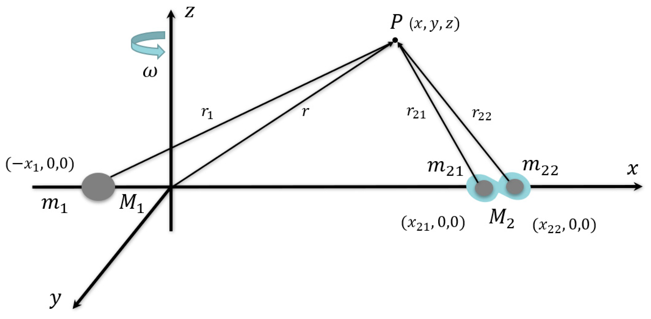
We investigate a planar CRTBP in which two massive bodies, $M_1$ and $M_2$ (the primaries, with masses $m_1$ and $m_2$, respectively), move under their mutual gravitational attraction. At the initial time, both bodies are aligned along the horizontal $Ox$-axis, with $M_2$ positioned on the positive $Ox$-axis. The system is confined to the same plane and an additional infinitesimal body of mass $m$ moves within this plane, influenced by the gravitational attraction of the primaries. However, due to its negligible mass, it does not perturb their motion. Unlike the classical restricted three-body problem, the secondary body $M_2$ is not a single mass but rather a dipole system consisting of two identical components, $m_{21}$ and $m_{22}$, separated by a fixed distance $d$. The total mass of the dipole is given by $m_2=m_{21}+m_{22}$. Defining $\nu$ as the mass parameter, we set $m_{21}=m_{22}=\nu$. Let also $r_1$, $r_{21}$ and $r_{22}$ be the respective distances of $m_1, m_{21}$ and $m_{22}$ from the infinitesimal body (see Figure 1). For simplicity, the system is described in a dimensionless framework. The unit of distance D is normalized to the separation between $M_1$ and the center of mass of the dipole $M_2$, and time, with ω⁻¹. Similarly, masses are scaled appropriately. In these canonical units, the total system mass, $M=m_1+m_2,$ is set to unity, leading to $m_1=1-m_{21}-m_{22}=1-2\nu$ with $m_2=2\nu$. The mass ratio satisfies the constraint $0<\nu =m_{21}/(m_1+m_{21}+m_{22})=m_{22}/(m_1+m_{21}+m_{22})\le 1/4$ where $m_1>>m_{21}=m_{22}$ [33]. Following the conventions established in [30,33], we describe the motion of the infinitesimal body within the rotating frame of the dipole system. The governing equations in three dimensions take the form:

$$\ddot{x}-2\dot{y}={\displaystyle \frac{\partial \Theta }{\partial x}}={\Theta }_x,\ddot{y}+2\dot{x}={\displaystyle \frac{\partial \Theta }{\partial y}}={\Theta }_y,\ddot{z}={\displaystyle \frac{\partial \Theta }{\partial z}}={\Theta }_z,$$

(1)

where the dots indicate derivatives with respect to time and the effective potential $\Theta$ in the co-rotating frame, expressed in synodic coordinates, given by:

$$\Theta (x,y,z)={\displaystyle \frac{x^2+y^2}{2}}+k\hspace{0.17em}\left({\displaystyle \frac{1-2v}{r_1}}+{\displaystyle \frac{v}{r_{21}}}+{\displaystyle \frac{v}{r_{22}}}\right),$$

(2)

in which

$$\begin{array}{c}{r}_1^2={(x+2v)}^2+y^2+z^2,r_{21}^2={(x+2v+f-1)}^2+y^2+z^2,\\ r_{22}^2={(x+2v-f-1)}^2+y^2+z^2,f={\displaystyle \frac{d}{2}}.\end{array}$$

(3)

In this context, the distances from the infinitesimal third body to the two primaries are denoted as $r_i\hspace{0.17em}(i=1,\hspace{0.17em}\hspace{0.17em}21,\hspace{0.17em}\hspace{0.17em}22)$ and the dimensionless parameter, $k=(GM)/({\omega }^2{D}^3)$, represents the ratio of gravitational to centrifugal forces, commonly known as the ‘force ratio’. The total mass refers to the combined mass of the two primaries, and the angular velocity, denoted by ω, describes their relative rotation. The distance between the two hypothetical point masses, that is, the length of the secondary body M₂ is denoted as d, and G is the gravitational constant with a value of $G=6.67408\times {10}^{-11}{\mathrm{m}}^3{\mathrm{kg}}^{-1}{\mathrm{s}}^{-2}$. When the force ratio equals one, the gravitational attraction between the two primaries balances the centrifugal force due to their rotation. For values of the force ratio less than one (fast rotation), the centrifugal force exceeds gravitational attraction, requiring tensile stress in the connecting rod to maintain the separation between the bodies. For values of the force ratio greater than one (slow rotation), compressive stress is needed in the rod to maintain a constant distance between the primaries [22,24]. Thus, the force ratio ranges from zero to infinity, i.e., $k\in (0,\infty ),$ with the case of a force ratio larger than one, i.e., $k>1,$ being more common. This is typically observed in binary asteroids where a squeezing force is present between the two components due to their slow rotation.

When the primary body $m_1$ is radiating with radiation coefficient $q_1$, the modified equations of motion of the third body with the allowance for the radiation force of the larger primary and rotating dipole secondary are finally written in the form [30]

$$\begin{array}{c}\ddot{x}-2\dot{y}={\displaystyle \frac{\partial \Theta }{\partial x}}={\Theta }_x=x-k\hspace{0.17em}\left[{\displaystyle \frac{q_1(1-2v)(x+2v)}{r_1^3}}+{\displaystyle \frac{v(x-1+2v+f)}{r_{21}^3}}+{\displaystyle \frac{v(x-1+2v-f)}{r_{22}^3}}\right],\\ \ddot{y}+2\dot{x}={\displaystyle \frac{\partial \Theta }{\partial y}}={\Theta }_y=y\hspace{0.17em}\left\{1-k\left[{\displaystyle \frac{q_1(1-2v)}{r_1^3}}+{\displaystyle \frac{v}{r_{21}^3}}+{\displaystyle \frac{v}{r_{22}^3}}\right]\right\},\\ \ddot{z}={\displaystyle \frac{\partial \Theta }{\partial z}}={\Theta }_z=kz\left[{\displaystyle \frac{q_1(1-2v)}{r_1^3}}+{\displaystyle \frac{v}{r_{21}^3}}+{\displaystyle \frac{v}{r_{22}^3}}\right]\end{array}$$

(4)

with

$$\Theta ={\displaystyle \frac{x^2+y^2}{2}}+k\hspace{0.17em}\left[{\displaystyle \frac{q_1(1-2v)}{r_1}}+{\displaystyle \frac{v}{r_{21}}}+{\displaystyle \frac{v}{r_{22}}}\right].$$

(5)

The energy-like integral (known as the Jacobi integral) of this problem is given by the expression:

$$C=2\Theta -{\vartheta }^2$$

(6)

with ${\vartheta }^2={\dot{x}}^2+{\dot{y}}^2+{\dot{z}}^2$, where C is the Jacobian constant. A considerable amount of literature has explored its use in analyzing possible motions, including the identification of stability or instability. The mass reduction factor on the particle (see, e.g., [5]) is given by the relation $q_1=1-b_1$, such that $0<q_1\le 1$, where $b_1$ is the radiation coefficient defined as $b_1=F_r/F_g,$ where $F_r$ is the force due to radiation and $F_g$ expresses the gravitational force. Note that an increase in radiation pressure leads to a decrease in the mass reduction factor, provided that the gravitational force remains unchanged. It should be noted that when the bigger primary does not radiate (namely, $q_1=1$), the equations of motion are the same as those in [30], while we obtain the gravitational restricted three-body problem when $k=1,$ and $d=f=0$ [1]. Recall here that the distance D between the more massive primary asteroid, treated as a radiation source, and the center of mass of the dipole body $M_2$, consisting of two hypothetical components, is assumed to be constant.

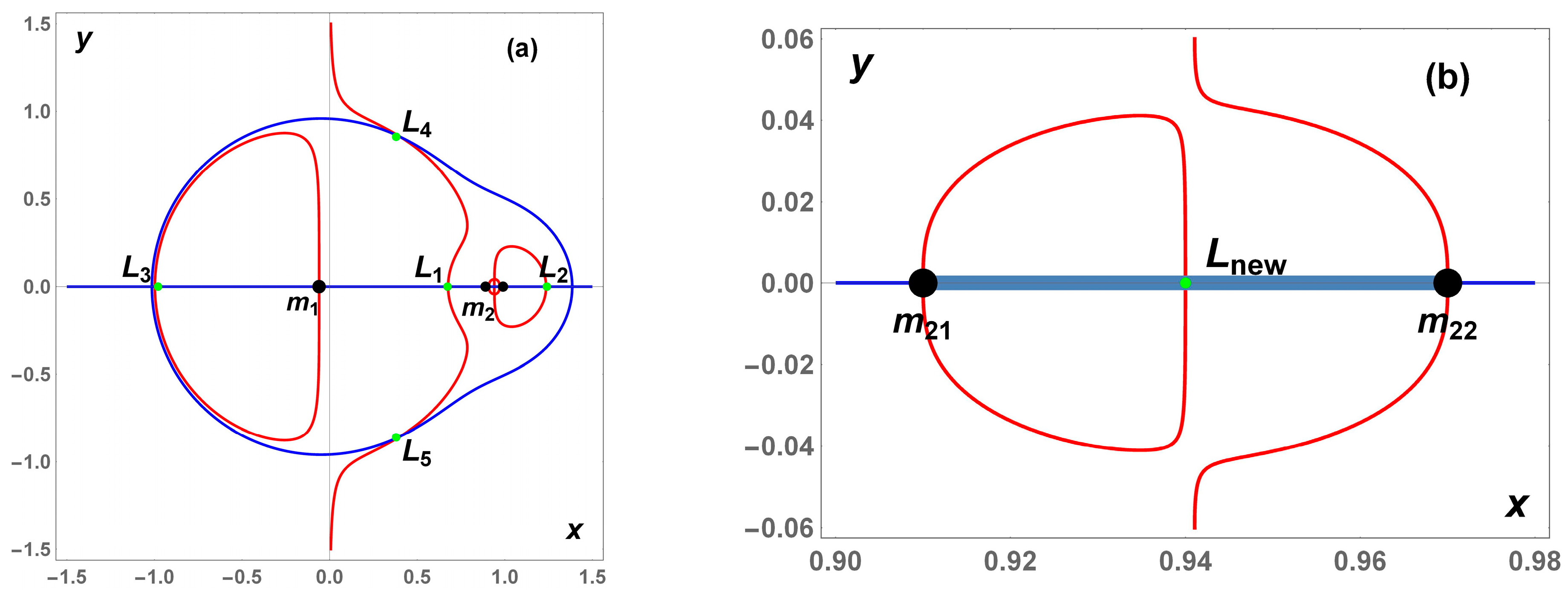
3. Existence and Location of the Equilibrium Points

The CRTBP is well known for having five equilibrium points (EPs). Three of these ($L_1,L_2,$ and $L_3$) are collinear and situated along the x-axis, while the remaining two $(L_4$ and $L_5)$ are non-collinear and lie off the x-axis. In the case of the CRTBP involving a rotating mass dipole, which represents an elongated rotating body, the number, location, and stability of these equilibrium points are further influenced by the mass parameter and the rotational effects of the secondary body [22,24,32,33]. Moreover, the introduction of photogravitational perturbations, such as radiation pressure from a radiating primary, adds further complexity to the system, making the characteristics of the equilibrium points highly sensitive to the radiation coefficient. In such systems, equilibrium points are classified as natural or artificial, where natural points arise from the intrinsic balance of gravitational, centrifugal, and radiation forces, while artificial points are established through continuous control forces, such as those generated by solar sails. As demonstrated by Zeng et al. [38,39], solar sails with variable lightness numbers enable spacecraft to achieve body-fixed hovering over elongated or irregular asteroids, positions that do not naturally exist in the gravitational potential alone.

In this study, we focus on analyzing the natural equilibrium points that emerge within the CRSTBP framework, incorporating both the radiative effects of the primary and the mass dipole influence of the secondary. We examine their existence, location, and stability, providing insights into the intrinsic dynamical structures that govern motion near binary asteroid systems. The equilibrium conditions are $\ddot{x}=\ddot{y}=\ddot{z}=0=\dot{x}=\dot{y}=\dot{z},$ such that the equilibrium points ${[x_0,y_0,z_0]}^{\mathrm{T}}$ are solutions to the equations:

$$\begin{array}{c}{x}_0-k\left({\displaystyle \frac{q_1(1-2v)(x_0+2v)}{r_{10}^3}}+{\displaystyle \frac{v(x_0-1+2v+f)}{r_{210}^3}}+{\displaystyle \frac{v(x_0-1+2v-f)}{r_{220}^3}}\right)=0,\\ y_0\left(1-k\left[{\displaystyle \frac{q_1(1-2v)}{r_{10}^3}}+{\displaystyle \frac{v}{r_{210}^3}}+{\displaystyle \frac{v}{r_{220}^3}}\right]\right)=0,\\ k{z}_0\left({\displaystyle \frac{q_1(1-2v)}{r_{10}^3}}+{\displaystyle \frac{v}{r_{210}^3}}+{\displaystyle \frac{v}{r_{220}^3}}\right)=0.\end{array}$$

(7)

Numerical analysis reveals that the equilibrium points are confined to the $xy-$plane, independent of the parameter values. For motion in the $xy-$plane ($z=0)$, the equilibrium points ($x_0,y_0$) in this dipole model are solutions to the equations:

$$\begin{array}{c}{x}_0-k\left({\displaystyle \frac{q_1(1-2v)(x_0+2v)}{r_{10}^3}}+{\displaystyle \frac{v(x_0-1+2v+f)}{r_{210}^3}}+{\displaystyle \frac{v(x_0-1+2v-f)}{r_{220}^3}}\right)=0,\\ y_0\hspace{0.17em}\left\{1-k\left[{\displaystyle \frac{q_1(1-2v)}{r_{10}^3}}+{\displaystyle \frac{v}{r_{210}^3}}+{\displaystyle \frac{v}{r_{220}^3}}\right]\right\}=0\end{array}$$

(8)

with

$$r_{10}=\sqrt{{(x_0+2v)}^2+y_0^2}, r_{210}=\sqrt{{(x_0+2v+f-1)}^2+y_0^2}, r_{220}=\sqrt{{(x_0+2v-f-1)}^2+y_0^2}.$$

(9)

From Equation (8), we observe that the existence, number, and position of stationary points vary with the magnitude of the mass ratio $v$, force ratio $k$, dipole distance $d$, and radiation pressure parameter $q_1$. Through numerical computations, we observed that the problem admits at most six EPs. Four of them are collinear, i.e., on the $x$-axis, which are posed on the positive axis between $M_1$ and $M_2$ ($L_1$), on the positive axis outside $M_2$ ($L_2$), on the negative axis outside $M_1$($L_3$), and the fourth one on the positive axis ($L_{new}$) located always at $1-2\nu$, i.e., at the center of $M_2$, and two of them are non-collinear ($L_{4(5)}$), away from the $x$-axis. The positions of the coordinates of the EPs on the ($x,y$) correspond to the intersections of the equations ${\Theta }_x=0$ (red curve) and ${\Theta }_y=0$ (blue curve). In Figure 2 we depict the locations of the equilibria, when $\nu =0.03$, $q_1=0.9$, $k=1.02$, and $d=0.06$.

We remark here that, in the case of irregularly shaped celestial bodies, such as asteroids or comets, the inner equilibrium points at the body’s center may hold significant relevance, since many of these bodies remain largely unexplored, with properties like surface composition and density inferred from indirect measurements [20]. Additionally, the nature and stability of the equilibrium points within these bodies can offer insights into their internal structures and stress distributions, potentially aiding in the study of their failure modes.

It should be pointed out that setting $d=0,\hspace{0.17em}\hspace{0.17em}{q}_1=1,\hspace{0.17em}\hspace{0.17em}k=1,$ the system degenerates to the classical RTBP with five equilibrium points obtained at similar positions with respect to the classical equilibrium points. The present dynamical system contains total four parameters determining the potential distribution of the modified dipole model: namely, the mass parameter $\nu$, the force ratio $k,$ the radiation parameter $q_1$ and the secondary mass dipole distance parameter $d$. Meanwhile, previous studies explained the presence of new additional equilibrium point in the dynamical system when $d\ne 0$ and considering $k=1$ (see, e.g., [32,33]). In this context, the present study investigates how the force ratio and radiation pressure parameters affect the positions and stability of equilibrium points, as well as the regions of motion accessible to the infinitesimal body. The permissible region for mass parameter $v$ is taken to be $v\in (0,0.25],$ region of radiation factor is $q_1\in (0,1],$ rotation of the asteroid is $k\in (0,10]$ while the mass dipole distance is $d\in (0,0.11]$.

In this section, we separately consider the effect of each one of these two parameters [$q_1$, $k$] on the positions of the classical five equilibrium points (but now there is also the fourth collinear point, $L_{new}$, located at $(1-2v,0).$ $L_{new}$ is located inside of the rotating dipole $M_2$ and suffers negligible effects from the elongation of the secondary body, force ratio of the primaries, and radiation pressure of the primary body, so the results related to this point are not shown here in detail and only other five equilibrium points are considered.

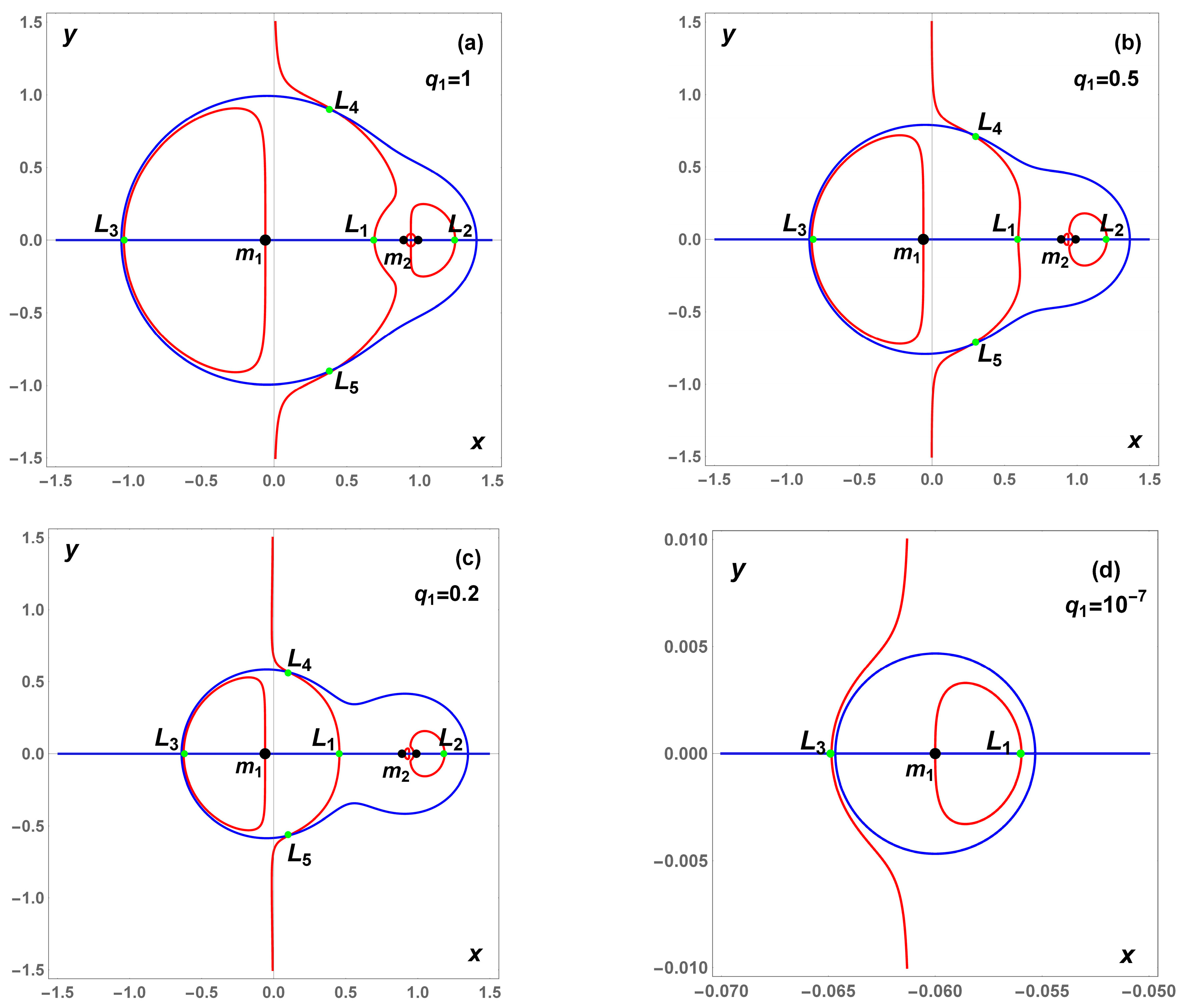
To explore the impact of radiation pressure on the equilibrium points’ positions, we analyze three distinct values of the radiation pressure factor; i.e., $q_1=1,\hspace{0.17em}\hspace{0.17em}{q}_1=0.5,$ and $q_1=0.2,$ when values of $v=0.03,$ $k=1.02,$ and $d=0.06$ are fixed. In Figure 3, this effect is shown. In frame (a), we consider the gravitational case $(q_1=1)$ while in the last two frames (frame b and frame c) we consider that the primary body radiates $(q_1=0.5$ and $q_1=0.2,$ correspondingly), so we can see how the radiation factor, $q_1,$ effects the dynamical problem. The equilibria $L_1,L_2,L_3,L_{4(5)}$ approach $m_1$, while $L_2$ approaches $m_2$ as the radiation factor increases. It is seen that the locations of the equilibrium points $L_1,L_3,L_{4(5)}$ are more sensitive to varying radiation pressure in the primary body, compared to $L_2$. When the parameter $q_1$ decreases (extreme radiation) the triangular (non-collinear) equilibria go to the massive primary $m_1$ along the Oy axis. In the same vein, our numerical calculations suggest that with the increase of $q_1$ the boundary value of $k$ for the existence of $L_{4(5)}$ decreases. For instance, for a value of $q_1$ = $0.0000001$, the non-collinear points $L_4$ and $L_5$ coincide on the collinear point $L_3$, and, therefore, the problem has then four collinear equilibrium points ($L_1$, $L_2$, $L_3$ and $L_{new}$). Panel 3d shows a zoom of the region close to the primary body $m_1$ where the equilibria $L_{4,5}$ disappear by coalescing at $L_3.$ A similar behavior is observed in the PCRTBP, where increasing radiation pressure factors (i.e., decreasing $q_{1,2}$ values) cause the triangular equilibrium points $(L_4,\hspace{0.17em}\hspace{0.17em}{L}_5)$ to move toward the inner collinear point. Eventually, they merge along the axis, transferring their stability to $L_1$ in the process [4].

In the gravitational CRTBP with elongated bodies triangular equilibrium points are only present for $k>0.125$ [22]. When $k<0.125$ the equilibrium point $L_1$ coincides with the positions of $L_4$ and $L_5.$ In the photogravitational version, where the primary body radiates, we find that for any $v\in (0,0.25]$ there are combinations of parameters $k$ and $q_1$ that enable the existence of non-collinear equilibrium points. Specifically, the critical value of k, at which $L_4$ and $L_5$ vanish, is influenced by $q_1$.

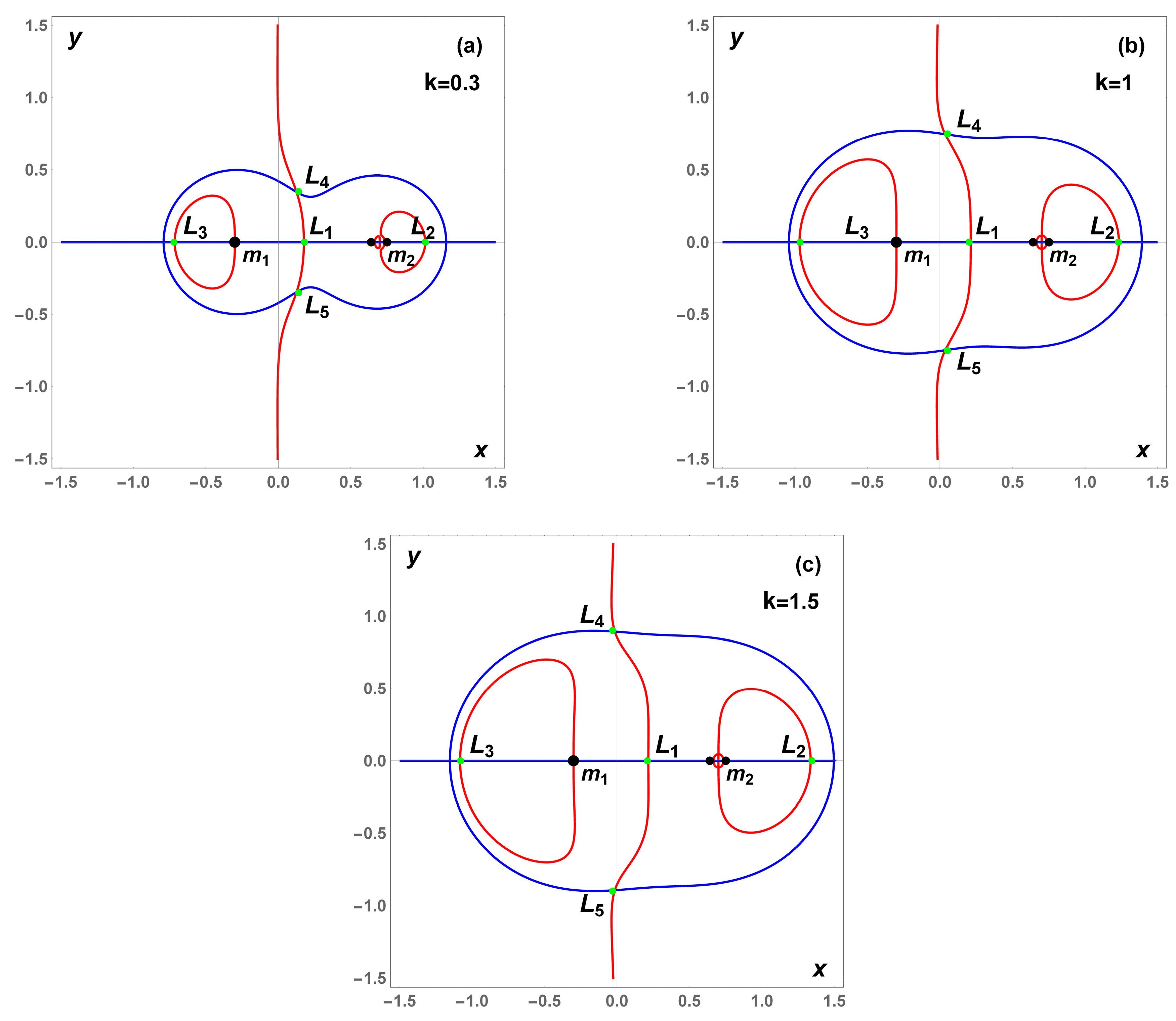
In Figure 4, the evolution of the five EPs of the problem for $v=0.15$, $d=0.065$, and $q_1=0.55$ and for several values of the force ratio k, are illustrated. This means that only the force ratio parameter k varies, i.e., for $k=0.3,$ $k=1,$ and $k=1.5,$ correspondingly. Figure 4, shows that $L_2$ and $L_3$ shift away from $m_2$ and $m_1,$ respectively, while $L_{4(5)}$ and $L_1$ increase from $m_1$ and the origin correspondingly as the force ratio increases. We remark that the effects of rotation rate (force ratio) of bodies on $L_2,L_3,L_{4(5)}$ are very significant, but does not essentially change the position of $L_1.$ Our numerical analysis reveals that, as $q_1$ approaches 0 for varying values of $k,$ the triangular points $L_4$ and $L_5$ gradually move towards $L_3$, eventually merging into a single point. Furthermore, in our study, four collinear equilibrium points, $L_1$, $L_2$, $L_3$ and $L_{new}$, are found to exist for all values of the parameter $k.$ Therefore, based on the analysis in Figure 4, we conclude that the force ratio plays a crucial role in determining both the existence and the positions of the equilibrium points.

4. Zero-Velocity Curves (ZVCs) in the ($\mathit{x}\mathbf{,}\mathit{y}$) Plane

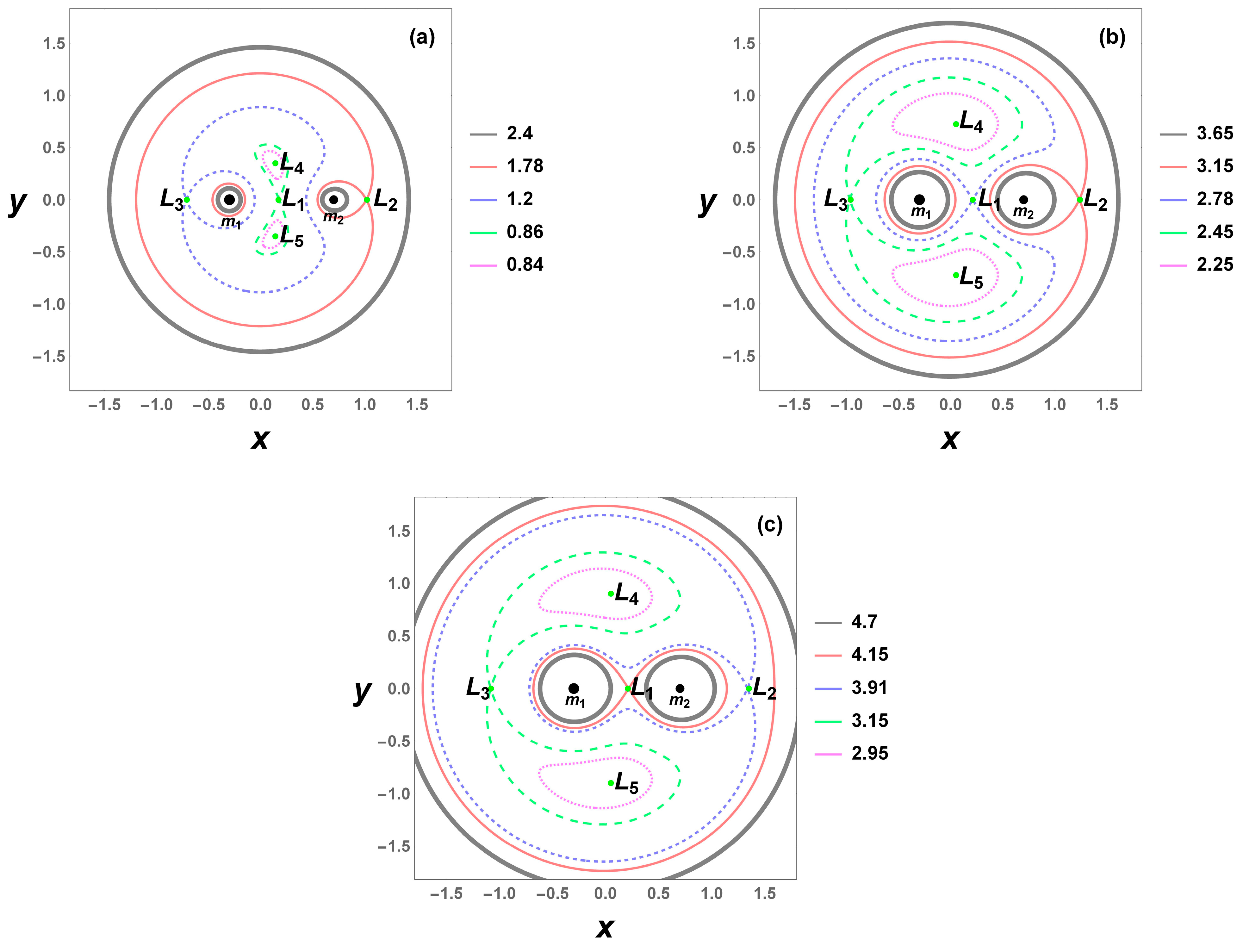
The contours of Relation (6) for zero velocity produce the zero velocity curves (ZVCs) of this problem. The resulting curves determine regions where the infinitesimal third body is permitted to move ($\vartheta \ge 0$) and where it is forbidden to move ($\vartheta <0$) for certain values of the Jacobi constant C. We now turn to illustrate the ZVCs in the ($x,y$) plane for several values of the radiation factor $q_1$ and force ratio $k$.

In Figure 5, we have plotted the ZVCs corresponding to the values of the Jacobian constant C computed at the collinear equilibrium points (red, blue, green curves) as well as to values of the Jacobian constant C slightly higher than the values of C computed at the non-collinear points (magenta curves) for fixed values of the parameters $\nu =0.03$, $d=0.06$, and $k=1.02$ when the bigger primary radiates. In all frames, ZVCs are classified from the larger to smaller value of the Jacobian constant C. In Figure 5a, we plot the ZVCs for $q_1=1$ (classical dipole model) and for $C=4.0,$ $C=C_{L1}\cong 3.52965,$ $C=C_{L2}\cong 3.42468,$ $C=C_{L3}\cong 3.09995$ and $C=C_{L4(5)}\cong 3.05$. We observe that the third body can move around the two primary bodies $m_1$ and $m_2$ only for $C<C_{L1}=3.52965$. In Figure 5b,c, we consider the cases when the primary body $m_1$ radiates. We present them for two values of the radiation factor, $q_1=0.5$ and $q_1=0.2,$ respectively. In the first case, we plot the curves for $C=3.3,$ $C=C_{L2}\cong 2.67785$, $C=C_{L1}\cong 2.17533$, $C=C_{L3}\cong 2.00327$, and $C=C_{L4(5)}\cong 1.95$. When $C<C_{L1}=2.17533,$ a channel is created joining the body $m_2$ and the third body can move from $m_2$ to $m_1$ and vice versa. In the second case, where we plot the ZVCs for $C=2.9,$ $C=C_{L2}\cong 2.21947$, $C=C_{L1}\cong 1.20506$, $C=C_{L3}\cong 1.14766$, and $C=C_{L4(5)}\cong 1.12$. We observe that the third body can move around the two primary bodies $m_1$ and $m_2$ only for $C<C_{L1}\cong 1.20506$. Note, symbol $\approx$ is used to state very small differences between the values of the corresponding Jacobian constants as long as these points exist in the figure. Also, we remark that the energy integral is a surface with C arbitrary constant and we choose such C in the figures, in order to obtain the appropriate projection of the surface on the $xy-$plane.

From the results in Figure 5, we can observe three main results. The first is that along with the increase of $q$ from 1 to 0.2 noticeable changes in the ZVCs can be found at the region between the primary bodies $m_1$ and $m_2,$ transforming from the nearly connected region to a more trapped area. The second is that between the collinear equilibrium points, the ZVCs form ovals of regions not allowed to motion, and shrink along with the increase of $q$ from 1 to 0.2. It is evident that the region surrounding the primary body remains more confined compared to that of the secondary. The third is that the third body can orbit the primaries at progressively lower values of the Jacobi constant C corresponding to the collinear equilibria, as radiation pressure increases. In particular, we note in the second and third frames that the ZVCs open firstly for $C<C_{L1}\cong 2.17533$ and $C<C_{L1}=1.20506,$ correspondingly, compared to the gravitational case (Figure 5a), which opens for $C<C_{L1}<3.52965$. Consequently, the permissible regions of motion for the infinitesimal body are highly sensitive to both the Jacobi constant and the radiation pressure factor.

Similarly, in Figure 6, we present the ZVCs corresponding to the exact values of the Jacobian constant C computed at the collinear equilibrium points (red, blue, green curves) as well as to values of C slightly higher than the values of C computed at the non-collinear points (magenta curves) for fixed values of the parameters $v=0.15,\hspace{0.17em}\hspace{0.17em}\hspace{0.17em}d=0.065,\hspace{0.17em}\hspace{0.17em}\hspace{0.17em}{q}_1=0.55$, and for three values of the rotation parameter $k$. In Figure 6a, we have ZVCs for $k=0.3$ (fast rotation) and $C=2.4,$ $C=C_{L2}\cong 1.78345,$ $C=C_{L3}\cong 1.19513,$ $C=C_{L1}\cong 0.861107$, and $C=C_{L4(5)}\cong 0.84$. We observe that the third body can move around the two primary bodies $m_1$ and $m_2$ only for $C<C_{L3}\cong 1.19513$. In Figure 6b, we have curves for $k=1$ (classical rotating mass dipole) and for $C=3.65,$ $C=C_{L2}\cong 3.15248,$ $C=C_{L1}\cong 2.7838,$ $C=C_{L3}\cong 2.44957$, and $C=C_{L4(5)}\cong 2.25$. In this case, only for $C<C_{L1}\cong 2.7838$ can the third body move from $m_1$ to $m_2$ and vice versa. Figure 6c shows the case for $k=1.5$ (slow rotation) and for $C=4.7,$ $C=C_{L1}\cong 4.15295,$ $C=C_{L2}\cong 3.90969,$ $C=C_{L3}\cong 3.15295$, and $C=C_{L4(5)}\cong 2.95$. And, in this case, only for $C<C_{L1}\cong 4.15295$ can the third body move from $m_1$ to $m_2$ and vice versa. In Figure 6, the topological structure changes significantly along with the increase of $k$ and we can observe three main results. First we observe that the third body can move from one primary to the other one only for $C<C_{L3}\cong 1.19513$ (Figure 6a), $C<C_{L1}\cong 2.7838$ (Figure 6b), and $C<C_{L1}\cong 4.15295$ (Figure 6c) as closed zero velocity are formed around each of the two primary bodies $m_{1,2}.$ The second is that, along with the increase in $k$ from 0.3 to 1.5, noticeable changes in the ZVCs can be found at the region between the primary bodies $m_1$ and $m_2,$ transforming from the trapped area to the nearly connected region. In particular, the nearly connected region varies in a small range of curves with $k=1,\hspace{0.17em}\hspace{0.17em}k=1.5\hspace{0.17em}\hspace{0.17em}\ge \hspace{0.17em}\hspace{0.17em}1$ (Figure 6b,c) compared to that with $k=0.3<1$ (Figure 6a). This shows that fast-spinning asteroids have greater impact on the regions not allowed to motion than the slow-spinning ones, comparing Figure 6a $(k=0.3)$ with Figure 6c $(k=1.5).$ The third is that the third body can orbit the primaries at progressively higher values of C corresponding to the collinear equilibria as force ratio parameter increases. We conclude that allowed regions of motion to the infinitesimal body strongly depends on the value of the Jacobi constant and the rotation rate (force ratio $k$).

5. Linear Stability of the Equilibrium Points

To analyze the stability of the EPs, we shift the coordinate system so that the origin coincides with $L_i$ by adopting small displacements ${\xi }_1,\hspace{0.17em}\hspace{0.17em}{\xi }_2$, and ${\xi }_3$ from the equilibrium points such that

$$x=x{L}_i+{\xi }_1,y=y{L}_i+{\xi }_2,z=z{L}_i+{\xi }_3,$$

where $x{L}_i,\hspace{0.17em}\hspace{0.17em}y{L}_i,\hspace{0.17em}\hspace{0.17em}z{L}_i$ represent the coordinates $(x_0,\hspace{0.17em}{y}_0,\hspace{0.17em}{z}_0)$ associated with the equilibrium point $L_i.$ The variational equations describing the linearized dynamics of small perturbations are expressed as:

$$\begin{gathered} {\ddot{\xi }}_1-2{\dot{\xi }}_2={\Theta }_{xx}^{(0)}{\xi }_1+{\Theta }_{xy}^{(0)}{\xi }_2+{\Theta }_{xz}^{(0)}{\xi }_3 \\ {\ddot{\xi }}_2+2{\dot{\xi }}_1={\Theta }_{yx}^{(0)}{\xi }_1+{\Theta }_{yy}^{(0)}{\xi }_2+{\Theta }_{yz}^{(0)}{\xi }_3 \\ {\ddot{\xi }}_3={\Theta }_{zx}^{(0)}{\xi }_1+{\Theta }_{zy}^{(0)}{\xi }_2+{\Theta }_{zz}^{(0)}{\xi }_3 \end{gathered}$$

(10)

while the involved partial derivatives are computed at the equilibrium points and are given by:

$$\begin{array}{c}{\Theta }_{xx}^{(0)}=1-k\left[{\displaystyle \frac{q_1(1-2v)}{r_{10}^3}}+{\displaystyle \frac{v}{r_{210}^3}}+{\displaystyle \frac{v}{r_{220}^3}}-{\displaystyle \frac{3q_1(1-2v){(x_0+2v)}^2}{r_{10}^5}}-{\displaystyle \frac{3v{(x_0+2v-1+f)}^2}{r_{210}^5}}-{\displaystyle \frac{3v{(x_0+2v-1-f)}^2}{r_{220}^5}}\right],\\ {\Theta }_{yy}^{(0)}=1-k\left[{\displaystyle \frac{q_1(1-2v)}{r_{10}^3}}+{\displaystyle \frac{v}{r_{210}^3}}+{\displaystyle \frac{v}{r_{220}^3}}-{\displaystyle \frac{3q_1{y}_0^2(1-2v)}{r_{10}^5}}-{\displaystyle \frac{3v{y}_0^2}{r_{210}^5}}-{\displaystyle \frac{3v{y}_0^2}{r_{220}^5}}\right],\\ {\Theta }_{xy}^{(0)}={\Theta }_{yx}^{(0)}=k\hspace{0.17em}\left[{\displaystyle \frac{3q_1{y}_0(1-2v)(x_0+2v)}{r_{10}^5}}+{\displaystyle \frac{3v{y}_0(x_0+2v-1+f)}{r_{210}^5}}+{\displaystyle \frac{3v{y}_0(x_0+2v-1-f)}{r_{220}^5}}\right],\\ {\Theta }_{zz}^{(0)}=k\hspace{0.17em}\left[-{\displaystyle \frac{q_1(1-2v)}{r_{10}^3}}-{\displaystyle \frac{v}{r_{210}^3}}-{\displaystyle \frac{v}{r_{220}^3}}+{\displaystyle \frac{3q_1{z}_0^2(1-2\nu )}{r_{10}^5}}+{\displaystyle \frac{3\nu z_0^2}{r_{210}^5}}+{\displaystyle \frac{3\nu z_0^2}{r_{220}^5}}\right],\\ {\Theta }_{xz}^{(0)}={\Theta }_{zx}^{(0)}=3z_{0}k\hspace{0.17em}\left[{\displaystyle \frac{q_1(1-2v)(x_0+2\nu )}{r_{10}^5}}+{\displaystyle \frac{\nu (x_0+2\nu -1+f)}{r_{210}^5}}+{\displaystyle \frac{\nu (x_0+2\nu -1-f)}{r_{220}^5}}\right],\\ {\Theta }_{yz}^{(0)}={\Theta }_{zy}^{(0)}=3y_0{z}_{0}k\hspace{0.17em}\left[{\displaystyle \frac{q_1(1-2v)}{r_{10}^5}}+{\displaystyle \frac{\nu }{r_{210}^5}}+{\displaystyle \frac{\nu }{r_{220}^5}}\right],\end{array}$$

(11)

where $r_{10},\hspace{0.17em}\hspace{0.17em}{r}_{210}$ and $r_{220}$ are

$$r_{10}=\sqrt{{(x_0+2v)}^2+y_0^2+z_0^2},r_{210}=\sqrt{{(x_0+2v+f-1)}^2+y_0^2+z_0^2},r_{220}=\sqrt{{(x_0+2v-f-1)}^2+y_0^2+z_0^2}.$$

We define the state variable vector of the third body with respect to the stationary points $\mathbf{X}={({\xi }_1,{\xi }_2,{\xi }_3,{\dot{\xi }}_1,{\dot{\xi }}_2,{\dot{\xi }}_3)}^T$, and write Equation (10) as

$$\dot{\mathbf{X}}=\mathrm{{\rm B}}\mathbf{X},$$

(12)

where the coefficient matrix $\mathrm{{\rm B}}$ is time-independent and can be written as

$$\mathrm{{\rm B}}={\left(\begin{array}{cc}{0}_{3\times 3}& I_{3\times 3}\\ {\Theta }_{3\times 3}& {\rho }_{3\times 3}\end{array}\right)}_{6\times 6}.$$

(13)

Here, $0_{3\times 3}$ and $I_{3\times 3}$ denote the $3\times 3$ zero matrix and identity matrix, respectively, while the remaining two matrices are defined as follows:

$$\Theta =\left(\begin{array}{ccc}{\Theta }_{xx}^{(0)}& {\Theta }_{xy}^{(0)}& {\Theta }_{xz}^{(0)}\\ {\Theta }_{xy}^{(0)}& {\Theta }_{yy}^{(0)}& {\Theta }_{yz}^{(0)}\\ {\Theta }_{xz}^{(0)}& {\Theta }_{yz}^{(0)}& {\Theta }_{zz}^{(0)}\end{array}\right) \mathrm{and} \rho =\left(\begin{array}{ccc}0& 2& 0\\ -2& 0& 0\\ 0& 0& 0\end{array}\right).$$

(14)

Due to the symmetry of the configuration with respect to the xy-plane, the equilibrium points lie on this plane and take the form $(x_0,y_0,0).$ Under this symmetry, the third equation of system (10), governing the motion in the z-direction, becomes independent of the in-plane variables ${\xi }_1$ and ${\xi }_2,$ depending solely on the parameters $q_1,\hspace{0.17em}\hspace{0.17em}\nu ,\hspace{0.17em}\hspace{0.17em}k$ and $d.$ This decoupling allows the system to be effectively reduced to four dimensions by eliminating the $z$ and $\dot{z}$ components. Consequently, all mixed second-order partial derivatives involving $z$ vanish at the equilibrium points, simplifying the stability analysis [30]. Hence, the characteristic equation of matrix $\mathrm{{\rm B}}$ (Equation (12)) or system (10) is

$${\lambda }^4+(4-{\Theta }_{xx}^{(0)}-{\Theta }_{yy}^{(0)})\hspace{0.17em}{\lambda }^2+{\Theta }_{xx}^{(0)}\hspace{0.17em}{\Theta }_{yy}^{(0)}-{[{\Theta }_{xy}^{(0)}]}^2=0,$$

(15)

and its eigenvalues are:

$${\lambda }_{1,2,3,4}=\pm {\displaystyle \frac{1}{\sqrt{2}}}\sqrt{-\tau \pm \sqrt{\Delta }},$$

(16)

with

$$\tau =4-{\Theta }_{xx}^{(0)}-{\Theta }_{yy}^{(0)},\Delta ={\tau }^2-4\delta \mathrm{and} \delta ={\Theta }_{xx}^{(0)}{\Theta }_{yy}^{(0)}-{[{\Theta }_{xy}^{(0)}]}^2.$$

(17)

According to the Lyapunov stability theorem, linear stability is achieved when all four roots of the characteristic equation for λ are purely imaginary. This implies that the characteristic equation has four eigenvalues of the form:

$${\lambda }_{1,2}=\pm i{\omega }_1,{\lambda }_{3,4}=\pm i{\omega }_2$$

(18)

with

$${\omega }_{1,2}={\displaystyle \frac{1}{\sqrt{2}}}\sqrt{\tau \mp \sqrt{\Delta }},$$

(19)

which will be shown through the following necessary, as well as sufficient, conditions:

$$\tau >0,\delta >0,{\tau }^2-4\delta >0.$$

(20)

We note that the quantities ${\Theta }_{xz}^{(0)}={\Theta }_{zx}^{(0)}={\Theta }_{yz}^{(0)}={\Theta }_{zy}^{(0)}=0,$ while ${\Theta }_{xy}^{(0)}={\Theta }_{yx}^{(0)}$ and obtain ${\Theta }_{xy}^{(0)}={\Theta }_{yx}^{(0)}=0$ for the collinear equilibrium points, while ${\Theta }_{xy}^{(0)}={\Theta }_{yx}^{(0)}\ne 0$ for the noncollinear equilibrium points.

In the present problem, the stability of the EPs depends on the specific values of the involved parameters, $v,k,q_1$ and $d$. In the classical rotating mass dipole problem $(q_1=1,d=0,k\ne 1)$, it has been demonstrated that the collinear EPs $L_2$ and $L_3$ are unstable for all values of the system parameters. In contrast, the stability of the collinear point $L_1$ and the triangular EPs $L_4$ and $L_5$ (when they exist) is conditional, depending on specific values of the mass parameter $\mu$ and force ratio $k$ [22,23]. We observed similar results in the classical synchronous RTBP with $q_1=1$, where the stability of the collinear and triangular EPs depends on the parameters $\mu$, $k$, and $d$ (for details see [29,30]), while, in the photogravitational version, we observe that the stability of the equilibria of the problem depends on the radiation coefficient $q_1$ of the larger primary body as well. So, we computed the stability zones around the EPs for the classical rotating dipole problem, and in order to compare it with the photogravitational case, we computed the stability when the radiation factor has large values.

The results of the eigenvalues of the collinear and non-collinear equilibria by varying $\nu$ and $k$ with and without radiation factor for fixed $d$ are presented in

Table 1. The eigenvalues ${\lambda }_i,i=1,2,3,4$ of Equation (15) and the corresponding exact positions $(x_0,0)$ of the equilibria $L_{\mathrm{1,2},3}$ and $L_{new}$ with $d=0.065$ under the effect of the mass parameter $0.01\le v\le 0.06$ and force ratio ($0.02\le k\le 0.125$) in the absence of radiation pressure ($q_1=1)$.

$\mathit{v}$	$\mathit{k}$	${\mathit{\lambda }}_{\mathit{i}}({\mathit{L}}_1)$	${\mathit{\lambda }}_{\mathit{i}}({\mathit{L}}_2)$	${\mathit{\lambda }}_{\mathit{i}}({\mathit{L}}_3)$	${\mathit{\lambda }}_{\mathit{i}}({\mathit{L}}_{\mathit{n}\mathit{e}\mathit{w}})$
0.01	0.02	$\pm$0.485471$i$, $\pm$0.912625$i$ (0.256185, 0)	$\pm$11.6517, $\pm$8.30946$i$ (1.02681, 0)	$\pm$0.457219, $\pm$1.06481$i$ ($-$0.283195, 0)	$\pm$12.1108, $\pm$8.63143$i$ (0.961516, 0)
0.015	0.03	$\pm$0.559980$i$, $\pm$0.878634$i$ (0.287227, 0)	$\pm$9.24592, $\pm$6.62634$i$ (1.02440, 0)	$\pm$0.520552, $\pm$1.082460$i$ ($-$0.32807, 0)	$\pm$11.1384, $\pm$7.94965$i$ (0.957301, 0)
0.02	0.04	$\pm$0.618543$i$, $\pm$0.845529$i$ (0.309877, 0)	$\pm$7.78302, $\pm$5.60821$i$ (1.02233, 0)	$\pm$0.570692, $\pm$1.09757$i$ ($-$0.364834, 0)	$\pm$11.71820, $\pm$8.35606$i$ (0.951504, 0)
0.03	0.06	$\pm$0.683643$i$, $\pm$0.800020$i$ (0.340864, 0)	$\pm$6.03445, $\pm$4.40113$i$ (1.01917, 0)	$\pm$0.649855, $\pm$1.12332$i$ ($-$0.425084, 0)	$\pm$15.1205, $\pm$10.7462$i$ (0.935939, 0)
0.04	0.08	$\pm$0.620575$i$, $\pm$0.844259$i$ (0.359839, 0)	$\pm$5.00557, $\pm$3.69984$i$ (1.01715, 0)	$\pm$0.713019, $\pm$1.14536$i$ ($-$0.475004, 0)	$\pm$19.5480, $\pm$13.8646$i$ (0.917758, 0)
0.05	0.1	$\pm$0.478653$i$, $\pm$0.915352$i$ (0.370495, 0)	$\pm$4.32134, $\pm$3.23976$i$ (1.01601, 0)	$\pm$0.766685, $\pm$1.16503$i$ ($-$0.51860, 0)	$\pm$24.2380, $\pm$17.1728$i$ (0.898618, 0)
0.06	0.125	$\pm$0.112331, $\pm$1.00419$i$ (0.379745, 0)	$\pm$3.78070, $\pm$2.88161$i$ (1.01793, 0)	$\pm$0.808138, $\pm$1.18078$i$ ($-$0.564339, 0)	$\pm$29.6026, $\pm$20.9600$i$ (0.879121, 0)

,

Table 2. The eigenvalues ${\lambda }_i,i=1,2,3,4$ of Equation (15) and the corresponding exact positions $(x_0,0)$ of the equilibria $L_{1,2,3}$ and $L_{new}$ with $d=0.065$ under the effect of the mass parameter $0.01\le v\le 0.06$ and force ratio ($0.02\le k\le 0.125$) when $q_1=0.5)$.

$\mathit{v}$	$\mathit{k}$	${\mathit{\lambda }}_{\mathit{i}}({\mathit{L}}_1)$	${\mathit{\lambda }}_{\mathit{i}}({\mathit{L}}_2)$	${\mathit{\lambda }}_{\mathit{i}}({\mathit{L}}_3)$	${\mathit{\lambda }}_{\mathit{i}}({\mathit{L}}_{\mathit{n}\mathit{e}\mathit{w}})$
0.01	0.02	$\pm$0.565554$i$, $\pm$0.875751$i$ (0.200642, 0)	$\pm$11.7304, $\pm$8.36464$i$ (1.02674, 0)	$\pm$0.510590, $\pm$1.07957$i$ ($-$0.22762, 0)	$\pm$12.1969, $\pm$8.69179$i$ (0.961448, 0)
0.015	0.03	$\pm$0.706048$i$, $\pm$0.781683$i$ (0.223964, 0)	$\pm$9.33916, $\pm$6.69141$i$ (1.02425, 0)	$\pm$0.580955, $\pm$1.10079$i$ ($-$0.26471, 0)	$\pm$11.2265, $\pm$8.01143$i$ (0.957184, 0)
0.02	0.04	$\pm$0.116592$\pm$0.759696$i$) (0.240651, 0)	$\pm$7.886700, $\pm$5.68017$i$ (1.02206, 0)	$\pm$0.636669, $\pm$1.11888$i$ ($-$0.295389, 0)	$\pm$11.7928, $\pm$8.40840$i$ (0.951365, 0)
0.03	0.06	$\pm$(0.174514$\pm$0.777998$i$) (0.262774, 0)	$\pm$6.15108, $\pm$4.48115$i$ (1.01856, 0)	$\pm$0.724673, $\pm$1.14956$i$ ($-$0.346276, 0)	$\pm$15.1617, $\pm$10.7752$i$ (0.935816, 0)
0.04	0.08	$\pm$(0.188341$\pm$0.783578$i$) (0.275559, 0)	$\pm$5.12859, $\pm$3.78318$i$ (1.01607, 0)	$\pm$0.794924, $\pm$1.17571$i$ ($-$0.389045, 0)	$\pm$19.5705, $\pm$13.8805$i$ (0.917662, 0)
0.05	0.1	$\pm$(0.174412$\pm$0.777958$i$) (0.281992, 0)	$\pm$4.44699, $\pm$3.32375$i$ (1.01435, 0)	$\pm$0.854620, $\pm$1.19898$i$ ($-$0.426869, 0)	$\pm$24.2511, $\pm$17.1821$i$ (0.898541, 0)
0.06	0.125	$\pm$(0.058653$\pm$0.748955$i$) (0.287716, 0)	$\pm$3.90958, $\pm$2.96645$i$ (1.01549, 0)	$\pm$0.900437, $\pm$1.21745$i$ ($-$0.466468, 0)	$\pm$29.6103, $\pm$20.9655$i$ (0.879059, 0)

,

Table 3. The eigenvalues of Equation (15) and the corresponding exact positions $(x_0,\pm y_0)$ of the equilibria $L_{4\left(5\right)}$ with $d=0.065$ under the effect of the mass parameter $0.01\le v\le 0.1$ and force ratio ($0.3\le k\le 10$) in the absence of radiation force.

$\mathit{v}({\mathit{q}}_1=1)$	$\mathit{k}$	${\mathit{L}}_{4,5}({\mathit{x}}_0,\pm {\mathit{y}}_0)$	${\mathit{\lambda }}_{1,2},{\mathit{\lambda }}_{3,4}$
0.0192	1.0	$(0.462018, \pm$0.865808)	$\pm$0.68485$\mathit{i}$,$\pm$0.728684$\mathit{i}$
0.01925	1.2	$(0.461993, \pm$0.937439)	$\pm$0.597425$\mathit{i}$,$\pm$0.801925$\mathit{i}$
0.0193	1.25	$(0.461909, \pm$0.953903)	$\pm$0.586432$\mathit{i}$,$\pm$0.809998$\mathit{i}$
0.0194	2	$(0.461862, \pm$1.15619)	$\pm$0.481409$\mathit{i}$,$\pm$0.876496$\mathit{i}$
0.038521	5	($0.423832, \pm$1.63500)	$\pm$0.526063$\mathit{i}$,$\pm$0.850446$\mathit{i}$
0.1	10	$(0.301045, \pm$2.09543)	$\pm$(0.14477 $\pm$ 0.721774$i$)

and

Table 4. The eigenvalues of Equation (15) and the corresponding exact positions $(x_0,\pm y_0)$ of the equilibria $L_{4\left(5\right)}$ with $d=0.065$ under the effects of the mass parameter $0.01\le v\le 0.1$ and force ratio ($0.3\le k\le 10$) in the presence of radiation force.

$\mathit{v}({\mathit{q}}_1=0.5)$	$\mathit{k}$	${\mathit{L}}_{4,5}({\mathit{x}}_0,\pm {\mathit{y}}_0)$	${\mathit{\lambda }}_{1,2},{\mathit{\lambda }}_{3,4}$
0.010	0.3	$(0.39624, \pm$0.330258)	$\pm$0.433348$\mathit{i}$,$\pm$0.901227$\mathit{i}$
0.0192	1.0	$(0.276612, \pm$0.728536)	$\pm$ (0.120615 $\pm$ 0.717320$i$)
0.01925	1.2	$(0.252689, \pm$0.791597)	$\pm$ (0.069683 $\pm$ 0.710532$i$)
0.0193	1.25	$(0.246844, \pm$0.805955)	$\pm$ (0.053151 $\pm$ 0.709102$i$)
0.0194	2	$(0.167840, \pm$0.978439)	$\pm$0.530781$\mathit{i}$,$\pm$0.847509$\mathit{i}$
0.038521	5	($-0.117335, \pm$1.35665)	$\pm$0.568223$\mathit{i}$,$\pm$0.822874$\mathit{i}$
0.1	10	($-0.557646, \pm$1.67229)	$\pm$(0.149409 $\pm$ 0.722719$i$)

. Table 1 and Table 2 show the four roots ${\lambda }_i,i=1,2,3,4$ of the collinear equilibrium points for $q_1=1$ and $q_1=0.5$, respectively, with $d=0.065$ for the range of the mass parameter $0.01\le v\le 0.06$, and the force ratio ($0.02\le k\le 0.125$). In this case, for every value of system parameters $v,k,d$, and $q_1$, the equilibrium points $L_2,L_3$, $L_{new}$ are always linearly unstable since, for the equilibria ($L_2,L_3$, $L_{new}$), the characteristic Equation (15) has two real eigenvalues ${\lambda }_{\mathrm{1,2}}=\pm a$ (causing the instability of the equilibria) and the other two are purely imaginary, i.e., ${\lambda }_{\mathrm{3,4}}=\pm ib$, where $a$ and $b$ are real numbers while in contrary, there are values of the problem parameters where the inner collinear point $L_1$ becomes stable due to pure imaginary roots (boldface roots). Our analysis reveals that the model parameter $k$, $v$ and $q_1$ significantly contribute to the reduction of the stability zone area. The progressive shrinkage of the stability region, mainly for positive values of $k$, from the gravitational case (third column of Table 1) to the photogravitational case (third column of Table 2) when the radiation factor has large values, is apparent. In particular, due to the radiation pressure, the stability part of the collinear equilibrium point $L_1$ decreases where the range of $k$ drops from $0.1\le k\le 0.02$, when $q_1=1$ to $0.03\le k\le 0.02$, and when $q_1=0.5$.

An examination of the results in Table 1 and Table 2 leads to the conclusion that the stability of EPs $L_2,L_3$, $L_{new}$ remains unaffected by the radiation pressure from the primary body $m_1$, and these points remain unstable across all values of the radiation parameter $q_1$. However, strong radiation pressure from $m_1$ increases the unstable region surrounding the collinear equilibrium point $L_1$, expanding it compared to the case where radiation pressure is absent over a wide range of $k$ and $v$.

Similarly, in Table 3 and Table 4, the characteristic roots of non-collinear equilibrium point $L_{4(5)}$ for $q_1=1$ and $q_1=0.5$, respectively, are presented for the range of mass parameter $0.01\le v\le 0.1$ and force ratio in the interval $0.3\le k\le 10$ when $d=0.065$. The idea is to be able to discern the effects of these parameters ($k$, $q_1$, $v$) on the stability outcome of the non-collinear points. From results in Table 3 and Table 4 we observe that stable zone for $L_{4(5)}$ decreases as the radiation pressure increases (i.e., $q_1$ decreases) when increasing both the mass and force ratio parameters of the primaries. In particular, the unstable zone is larger when the primary body is a radiation source with $q_1=0.5$ than when it is not ($q_1=1$). This shows that the radiation pressure is a destabilizing force. Moreover, we know from the classical RTBP that the triangular points are stable when $\mu \le {\mu }_{crit}=0.038520$ [1]. In the present case (photogravitational rotating dipole problem), we observe from Table 3 and Table 4 that when $\nu =0.038521$, all eigenvalues are imaginary quantities (stable motion). However, numerical computations show that when $k=1$ (only the gravitational interaction between the two primaries exists) there are two real eigenvalues, ${\lambda }_{\mathrm{1,2}}=\pm a$, (responsible for the equilibria’s instability) and two imaginary eigenvalues, ${\lambda }_{\mathrm{3,4}}=\pm ib$. This shows that the force ratio is a stabilizing force.

Based on the results presented in Table 1, Table 2, Table 3 and Table 4, we conclude that the linearization around the equilibrium points $L_2,\hspace{0.17em}\hspace{0.17em}{L}_3$, and $L_{new}$ yields two real eigenvalues (saddle) and two purely imaginary eigenvalues (center), indicating the presence of a two-dimensional stable manifold and a two-dimensional unstable manifold. In contrast, the behavior around $L_1$ and $L_{4(5)}$ varies depending on the system parameters. Specifically, for most cases in Table 1, there are two pairs of purely imaginary eigenvalues, corresponding to a four-dimensional stable manifold. Table 2, however, presents cases where complex saddle-type behavior emerges, with eigenvalues typically taking the form ${\lambda }_{1,2,3,4}=\pm a\pm ib.$ In some instances, a pair of real eigenvalues and a pair of imaginary eigenvalues coexist, further enriching the system’s dynamical structure. For the triangular equilibria $L_{4(5)},$ most cases also yield two pairs of purely imaginary eigenvalues, as shown in Table 3. However, in certain parameter regimes (Table 4), a complex saddle-type structure emerges, similar to that observed at $L_1.$ This highlights that changes in system parameters significantly impact the topology and stability of the phase space near these points, particularly around $L_1$ and $L_{4(5)}.$ For the spatial problem, the characteristic equation governing the linearized system near the equilibrium points is given by (see, e.g., [40]):

$$({\lambda }^2-{\Theta }_{zz}^{(0)})({\lambda }^4+(4-{\Theta }_{xx}^{(0)}-{\Theta }_{yy}^{(0)}){\lambda }^2+{\Theta }_{xx}^{(0)}{\Theta }_{yy}^{(0)}-{({\Theta }_{xy}^{(0)})}^2)=0$$

and the resulting eigenvalues determine the linear stability or instability of each equilibrium point. We computed the eigenvalues of this characteristic equation for the cases presented in Table 1, Table 2, Table 3 and Table 4 and observed that the nature of the eigenvalues is not influenced by the $z$-direction, confirming the decoupling of out-of-plane motion. In general, for $L_2,\hspace{0.17em}\hspace{0.17em}{L}_3$, and $L_{new},$ the eigenvalues are of the form $\pm a,\hspace{0.17em}\hspace{0.17em}\pm ib,\hspace{0.17em}\hspace{0.17em}\pm ic$, indicating a typical center $\times$ center $\times$ saddle structure. For $L_1,$ the system exhibits either purely imaginary eigenvalues of the form $\pm ia,\hspace{0.17em}\hspace{0.17em}\pm ib,\hspace{0.17em}\hspace{0.17em}\pm ic$ corresponding to a center $\times$ center $\times$ center configuration or a combination of real and imaginary eigenvalues $\pm a,\hspace{0.17em}\hspace{0.17em}\pm ib,\hspace{0.17em}\hspace{0.17em}\pm ic,$ leading to a center $\times$ center $\times$ saddle behavior. The triangular equilibrium points $L_{4(5)}$ mostly present a center $\times$ center $\times$ center structure with eigenvalues $\pm ia,\hspace{0.17em}\hspace{0.17em}\pm ib,\hspace{0.17em}\hspace{0.17em}\pm ic,$ but under certain parameter variations, they exhibit a center $\times$ complex saddle behavior characterized by eigenvalues of the form $\pm ia,\hspace{0.17em}\hspace{0.17em}\pm b\pm ic.$ For brevity, detailed eigenvalue computations are not displayed in the paper.

6. Periodic Orbits Around the Collinear Points

The study of periodic orbits in dynamical systems involving irregular gravitational fields is essential for understanding local stability and guiding mission design near asteroids and small bodies. Previous works, such as the investigation of periodic orbits around the dipole segment model for dumbbell-shaped asteroids [41], have demonstrated how simplified models can capture key dynamical features, including orbit shapes, stability, and bifurcation behavior. Similarly, periodic orbits near irregularly shaped asteroids have been studied using indirect optimal control methods, which identify families of periodic solutions, such as Lyapunov orbits and inclined orbits, in the gravitational field approximated by a rotating mass dipole [42]. These studies reinforce the crucial role of periodic orbit analysis in expanding the practical applications of simplified models to complex asteroid systems. In this context, our work extends the exploration of periodic orbits in the photogravitational restricted synchronous three-body problem with a mass dipole secondary, providing further insight into the stability and dynamical structure of such systems.

In particular, we investigate periodic motion in the vicinity of collinear equilibrium points within the context of the asteroid system 2001SN₂₆₃. To this end, we conduct a numerical investigation of the well-known Lyapunov families of periodic orbits that emerge from the collinear Lagrange points $L_1,$ $L_2,$ and $L_3$, as well as the additional equilibrium point $L_{new}.$ To ensure a precise characterization of the dynamical environment, we adopt particular values for the mass parameter and the distance between the components of the rotating mass dipole. Given the complex gravitational interactions present in the system, our numerical investigation aims to explore the intricate dynamical structures and their dependence on key physical parameters. In particular, we systematically vary both the radiation parameter and the force ratio parameter to assess their influence on the stability and evolution of periodic orbits. This approach provides deeper insights into how these factors shape the dynamical properties of the system, ultimately contributing to a more comprehensive understanding of the motion around equilibrium points in asteroid systems.

More precisely, the triple asteroid system 2001SN₂₆₃ consists of three gravitationally bound bodies designated as Alpha, Beta, and Gamma, in order of decreasing mass. Alpha, the dominant central body, has a diameter of 2.6 km, while its two smaller companions Beta and Gamma measure 0.78 km and 0.58 km in diameter, respectively, and orbit Alpha [43]. In this study, we focus on the Alpha–Gamma-spacecraft system as a practical application of our mathematical model, given that Gamma is an elongated body exhibiting synchronous rotation while Beta, being more distant from the other two central bodies, is neglected in our analysis [29]. For this system, we assume that Alpha acts as the primary radiation source, while Gamma, due to its irregular shape, is modeled as a rotating mass dipole. Following [44,45], we adopt a mass parameter of $\nu =0.005287$ and set the dipole separation distance to $d=0.186645$. The system’s short orbital period suggests it is in a minimal energy state [46]. However, in our model, the parameter $k$ deviates slightly from one due to the non-spherical nature of the binary asteroid system. This deviation aligns with the general behavior of most elongated binary asteroids, which tend to rotate slowly and experience internal forces that generate a compressive effect between the system’s components. The specific case where $k=1$ represents the situation for slow rotating asteroids, such as 2001SN₂₆₃, which can be described within the framework of the restricted synchronous three-body problem [45]. To further investigate the system’s dynamical behavior, we analyze the motion of a test particle in the vicinity of 2001SN₂₆₃ while varying the radiation pressure factor $q_1$ as well as the force ratio parameter.

One of the fundamental properties of periodic orbits is their stability as it plays a crucial role in determining the overall dynamical behavior of a system. Stability analysis provides insights into the long-term evolution of trajectories, the feasibility of maintaining orbits and the sensitivity of motion to perturbations. In the context of the considered model, to study the stability of a periodic orbit we set $x_1=x, { x}_2=y, x_3=\dot{x}$, and $x_4=\dot{y},$ thus, the equations of motion (4) are written in the following compact form:

$${\dot{x}}_i=f_i(x_1,x_2,x_3,x_4),\hspace{1em}i=1,2,3,4.$$

(21)

In the four-dimensional phase space, the motion of the third body is entirely determined by its initial conditions and the evolution of time. This implies that for any given solution, the coordinates of the third body are uniquely defined as functions of both its starting position and velocity, i.e.,:

$$x_i=x_i(x_{01},x_{02},x_{03},x_{04};\hspace{0.17em}\hspace{0.17em}t),\hspace{1em}i=1,2,3,4.$$

(22)

The partial derivatives of these coordinates with respect to the initial conditions satisfy the equations of variation, which describe how small perturbations in the initial state propagate over time (see, e.g., [47]). These derivatives provide essential information about the system’s local stability and sensitivity to initial perturbations, and they are expressed in the form:

$${\displaystyle \frac{\mathrm{d}}{\mathrm{dt}}}(v_{ij})={\displaystyle \frac{\mathrm{d}}{\mathrm{dt}}}\left({\displaystyle \frac{\partial x_i}{\partial x_{0j}}}\right)={\displaystyle \sum _{k=1}^4\frac{\partial f_i}{\partial x_k}\hspace{0.17em}\frac{\partial x_k}{\partial x_{0j}}},\hspace{1em}i,\hspace{0.17em}\hspace{0.17em}j=1,2,3,4,$$

(23)

where $f_{ij}=\partial f_i/\partial x_{0j},$ which are given by

$$\begin{array}{c}{f}_{31}=1-k\left[{\displaystyle \frac{q_1(1-2\nu )}{r_1^3}}+{\displaystyle \frac{\nu }{r_{21}^3}}+{\displaystyle \frac{\nu }{r_{22}^3}}-{\displaystyle \frac{3q_1(1-2\nu ){(x_1+2\nu )}^2}{r_1^5}}\right.\hfill \\ \left.\hspace{1em}\hspace{1em}\hspace{1em}\hspace{1em}\hspace{1em}\hspace{1em}\hspace{1em}\hspace{1em}\hspace{0.33em}\hspace{0.33em}-{\displaystyle \frac{3\nu {(-2+4\nu +d+2x_1)}^2}{4r_{21}^5}}-{\displaystyle \frac{3\nu {(2-4\nu +d-2x_1)}^2}{4r_{22}^5}}\right],\hfill \\ f_{32}=f_{41}={\displaystyle \frac{3}{2}}k\hspace{0.17em}{x}_2\left[{\displaystyle \frac{2q_1(1-2\nu )(x_1+2\nu )}{r_1^5}}+{\displaystyle \frac{\nu (-2+4\nu +d+2x_1)}{r_{21}^5}}+{\displaystyle \frac{\nu (-2+4\nu -d+2x_1)}{r_{22}^5}}\right],\\ f_{42}=1-k\left[{\displaystyle \frac{q_1(1-2\nu )}{r_1^3}}+{\displaystyle \frac{\nu }{r_{21}^3}}+{\displaystyle \frac{\nu }{r_{22}^3}}-{\displaystyle \frac{3q_1(1-2\nu )x_2^2}{r_1^5}}-{\displaystyle \frac{3\nu x_2^2}{r_{21}^5}}-{\displaystyle \frac{3\nu x_2^2}{r_{22}^5}}\right],\end{array}$$

and $f_{13}=1,$ $f_{24}=1,$ $f_{43}=-2,$ $f_{34}=2,$ while all the remaining partial derivatives are zero. The corresponding variations $v_{ij}$ for any orbit can be computed by integrating system (23) together with the equations of motion (4) of the problem. For the horizontal stability of a symmetric periodic orbit, we use the formulae which were introduced in [48] and are given by:

$$\begin{array}{c}{a}_h={\displaystyle \frac{\partial x_1}{\partial x_{01}}}+{\displaystyle \frac{\partial x_1}{\partial x_{04}}}{D}_{14},\hspace{1em}{b}_h={\displaystyle \frac{\partial x_1}{\partial x_{03}}},\\ c_h={\displaystyle \frac{\partial x_3}{\partial x_{01}}}-\left({\displaystyle \frac{\partial x_2}{\partial x_{01}}}+{\displaystyle \frac{\partial x_2}{\partial x_{04}}}{D}_{14}\right)\hspace{0.17em}(2+D_{14})+{\displaystyle \frac{\partial x_3}{\partial x_{04}}}{D}_{14},\hspace{1em}{d}_h={\displaystyle \frac{\partial x_3}{\partial x_{03}}}-{\displaystyle \frac{\partial x_2}{\partial x_{03}}}(2+D_{14}),\end{array}$$

(24)

where $x_0=(x_0,y_0,{\dot{x}}_0,{\dot{y}}_0)=(x_{01},0,0,x_{04})$ is the initial state vector of this orbit and $C_0=C(x_0)$ is the value of the Jacobi constant evaluated at this initial condition while we have set for abbreviation:

$$D_{14}=-{\displaystyle \frac{1}{2x_{04}}}\hspace{0.17em}{\displaystyle \frac{\partial C_0}{\partial x_{01}}}.$$

A periodic orbit is stable if $|(a_h+d_h)/2|\hspace{0.17em}\hspace{0.17em}<\hspace{0.17em}\hspace{0.17em}1,$ while it is unstable if $|(a_h+d_h)/2|\hspace{0.17em}\hspace{0.17em}>\hspace{0.17em}\hspace{0.17em}1$. In the case of symmetrical orbits, it holds $a_h=d_h,$ so they become $\left|a_h\right|\hspace{0.17em}\hspace{0.17em}<\hspace{0.17em}\hspace{0.17em}1$ and $\left|a_h\right|>1,$ respectively. The condition $a_h{d}_h-b_h{c}_h=1$ must hold for the property of area preservation.

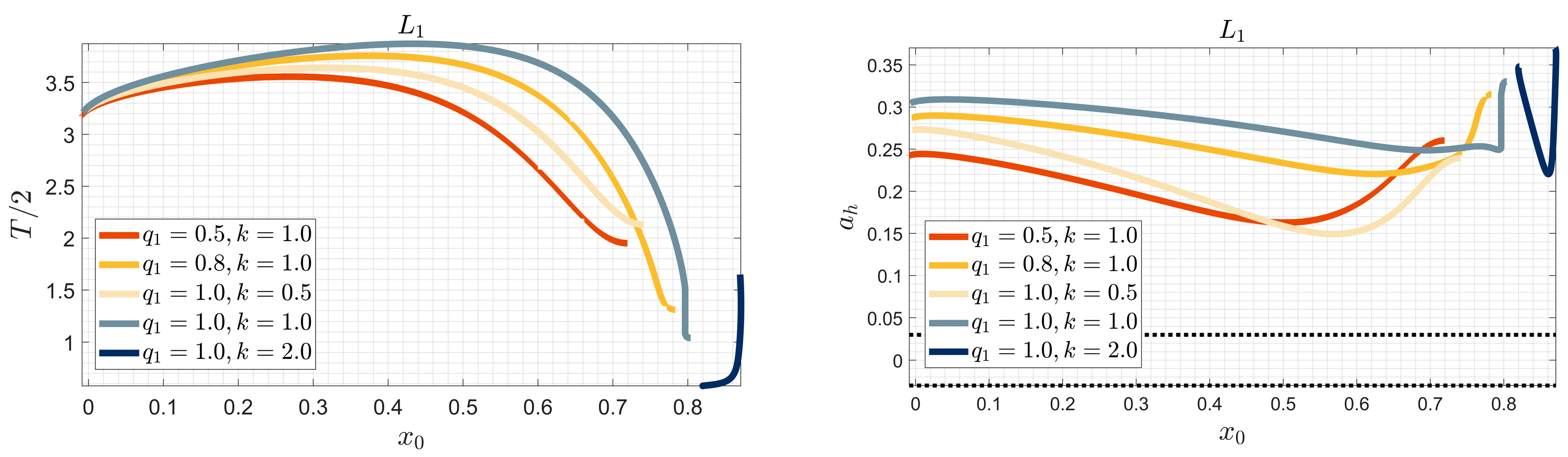
In Figure 7 we present our numerical results. Each subplot of this figure shows the characteristic curves (blue lines) of the Lyapunov families emanating from the three classical collinear equilibrium points $(L_1,\hspace{0.17em}{L}_2,\hspace{0.17em}{L}_3)$ and the newly identified collinear equilibrium point $(L_{new})$ in the context of the considered model. These curves are plotted in the plane of initial conditions $(C,x_0),$ illustrating the evolution of periodic orbits under different parameter values. The shaded gray regions correspond to the case where motion is not allowed for the spacecraft. Across all frames, the mass parameter ν and the dipole separation distance d remain fixed, ensuring that the results specifically correspond to the Alpha–Gamma-spacecraft system, as discussed previously. The top row of Figure 7, i.e., subplots (a)–(c), correspond to the scenario where the force ratio parameter is set to $k=1$. Within this configuration, the radiation pressure factor $q_1$ is varied to assess its influence on the system’s dynamics. Particularly, Figure 7a represents the case where no radiation pressure is exerted by the primary body $(q_1=1),$ meaning that only gravitational force is considered. Figure 7b and Figure 7c depict cases where the primary body acts as a radiation source, with $q_1=0.8$ and $q_1=0.5,$ respectively. In all three cases, the computed Lyapunov families terminate in collision orbits. Notably, the families originating from $L_2$ and $L_{new}$ reach these collision states at higher values of the Jacobi constant C (marked by purple asterisks) compared to those emerging from the other collinear points. Additionally, all families evolve in the plane of initial conditions with decreasing values of the initial coordinate $x_0.$ In the bottom row of Figure 7, subplots (d)–(e) explore the effect of varying the force ratio parameter k, while keeping $q_1=1,$ meaning the primary body does not radiate. Figure 7d examines a scenario where the force ratio parameter is halved $(k=0.5),$ representing case with a faster rotation rate compared to $k=1$. Figure 7e represents a case where the force ratio parameter is doubled $(k=2),$ corresponding to a more slowly rotating system. From these variations, we observe that in the slow rotation case $(k=2),$ the Lyapunov families emerging from $L_1$ and $L_{new}$ evolve differently compared to the other considered cases for the force ratio $(k\le 1).$ Unlike the families in the top row and in Figure 7d, which evolve by decreasing $x_0,$ the families now progress with increasing values of $x_0.$ This indicates a change in the dynamical structure of the system, emphasizing the role that rotational effects play in the evolution of periodic orbits.

In Figure 8, we present the evolution of all computed Lyapunov families in the $(x_0,T/2)$plane (left column), illustrating how the period varies as each family evolves for different parameter sets. The overall trend remains consistent across most cases, except for the fast rotation scenario $(k=2),$ where the families emanating from $L_1$ and $L_{new}$ deviate significantly from the expected pattern, as also observed in Figure 7. The right column of Figure 8 displays the horizontal stability diagrams corresponding to each computed family. Recall that a periodic orbit is considered stable if the stability parameter satisfies the inequality $\left|a_h\right|\hspace{0.17em}\hspace{0.17em}<\hspace{0.17em}\hspace{0.17em}1$. However, given the large variations in $a_h,$ we employ the transformation proposed in [49]:

$$y=\mathrm{sign}(x)\hspace{0.17em}{\displaystyle \frac{{\log }_{10}(1+|x|)}{{10}^c}},$$

where sign is the well-known sign function, and c is a tuning parameter (set to $c=1$ in our analysis). The transformed stability parameter allows for a clearer visualization of stability regions. From these diagrams, we observe that stability is only achieved in the families originating from the equilibrium point $L_3,$ while families emerging from the other equilibrium points remain unstable throughout their evolution.

Table 5. Numerical data for infinitesimal periodic orbits emanating from the four collinear equilibrium points for $k=1$, $d=0.186645$, and $\nu =0.005287$, for three specific values of the radiation factor.

Equilibrium	T/2	${\mathit{x}}_0$	${\dot{\mathit{y}}}_0$	${\mathit{x}}_{\mathit{c}}$	$\mathit{C}$	${\mathit{a}}_{\mathit{h}}$
$L_3$,    q1 $=1.0$	3.11294066	−1.00441654	0.00001	−1.00440663	3.01059472	1.583501
q1$=0.8$	3.11144635	−0.93305597	0.00001	−0.93304606	2.59773095	1.620177
q1$=0.5$	3.10813935	−0.79906566	0.00001	−0.79905577	1.90519652	1.701730
$L_1$,    q1 $=1.0$	1.04090545	0.80377752	0.00001	0.80377896	3.22846361	2015.905
q1$=0.8$	1.31000508	0.78314683	0.00001	0.78314909	2.73673041	1413.209
q1$=0.5$	1.95081242	0.71933363	0.00001	0.71933847	1.96190459	398.9715
$L_2$,    q1 $=1.0$	1.38083423	1.19157813	0.00001	1.19158064	3.19889714	1265.659
q1$=0.8$	1.21216205	1.18021722	0.00001	1.18021917	2.86805301	1625.211
q1$=0.5$	1.01290484	1.16733566	0.00001	1.16733703	2.36664937	2080.789
$L_{new}$,    q1 $=1.0$	0.83013618	0.98942554	0.00001	0.98942646	3.18442783	2501.843
q1$=0.8$	0.82315870	0.98257880	0.00001	0.98257970	2.78729566	2518.217
q1$=0.5$	0.77250787	0.97280621	0.00001	0.97280702	2.18653455	2630.117

and

Table 6. Numerical data for infinitesimal periodic orbits emanating from the four collinear equilibrium points for q₁ $=1.0$, $d=0.186645$, and $\nu =0.005287$, for three specific values of the force ratio parameter.

Equilibrium	T/2	${\mathit{x}}_0$	${\dot{\mathit{y}}}_0$	${\mathit{x}}_{\mathit{c}}$	$\mathit{C}$	${\mathit{a}}_{\mathit{h}}$
$L_3$,    k $=0.5$	3.10424853	−0.79851429	0.00001	−0.79850441	1.89926720	1.781956
k$=1.0$	3.11294066	−1.00441654	0.00001	−1.00440663	3.01059472	1.583501
k$=2.0$	3.12017578	−1.26391791	0.00001	−1.26390798	4.77400697	1.430961
$L_1$,    k $=0.5$	2.12928997	0.74146624	0.00001	0.74147190	1.91510911	247.0286
k $=1.0$	1.04090545	0.80377752	0.00001	0.80377896	3.22846361	2015.905
k$=2.0$	0.57825937	0.82119639	0.00001	0.82119683	5.79571119	3027.920
$L_2$,    k $=0.5$	0.87477363	1.14301149	0.00001	1.14301251	2.27331652	2400.457
k$=1.0$	1.38083423	1.19157813	0.00001	1.19158064	3.19889714	1265.659
k$=2.0$	2.30624641	1.33005350	0.00001	1.33006000	4.85541789	143.4740
$L_{new}$,    k $=0.5$	0.91503547	0.96151393	0.00001	0.96151505	2.06678270	2307.919
k$=1.0$	0.83013618	0.98942554	0.00001	0.98942646	3.18442783	2501.843
k$=2.0$	0.54311241	1.00584006	0.00001	1.00584047	5.37319771	3092.195

provide some representative initial conditions for the computed Lyapunov families corresponding to different parameter combinations. Specifically, each table presents the half-period of the orbit $T/2,$ along with the initial position and velocity components $(x_0,{\dot{y}}_0)$ at the first orbit’s perpendicular intersection with the Ox-axis. Note, at this intersection, the remaining components are set to zero; i.e., $y_0=0$ and ${\dot{x}}_0=0$. Additionally, we include the position component $x_c,$ from which we may define the orbit’s amplitude along the Ox-axis, as well as the corresponding Jacobi constant C and the horizontal stability parameter $a_h.$ Table 5 examines the influence of the radiation pressure factor $q_1$ on the infinitesimal periodic orbits while keeping the force ratio parameter fixed at $k=1$. The numerical results indicate variations in stability characteristics and Jacobi constant values as the radiation pressure changes. Table 6, on the other hand, explores the effect of different values of the force ratio parameter k while maintaining a constant radiation pressure factor $q_1=1$. The results highlight how variations in the rotational characteristics of the primary bodies affect the stability of periodic orbits. The data presented in both tables may serve as initial conditions for computing all the Lyapunov families examined in this study; therefore, they provide a valuable reference for analyzing them and assessing their stability properties across different parameter regimes.

7. Discussion

The dynamics of motion around equilibrium points in the modified synchronous circular restricted three-body problem (CRSTBP) were investigated, considering a radiating primary and a secondary modeled as a mass dipole. Unlike the classical three-body problem, the number and stability of collinear equilibrium points in this modified CRTBP are influenced by the perturbation parameters, namely, radiation pressure factor $q_1,$ force ratio k, and dipole strength d. Our analysis reveals the existence of six equilibrium points, particularly, four collinear with the primaries and two non-collinear. The parameters $q_1$ and k affect the existence and location of equilibrium points. Specifically, an increase in $q_1$ reduces the critical value of k required for the existence of the triangular equilibrium points $L_{4(5)}.$ Furthermore, as $q_1$ increases, the positions of $L_1,L_3$, and $L_{4(5)}$ shift toward the primary mass $m_1$, while, simultaneously, $L_2$ moves toward the secondary mass $m_2$. Regarding the force ratio k, we observe distinct trends in equilibrium displacement: $L_2$ and $L_3$ move away from $m_2$ and $m_1$, respectively, while $L_{4(5)}$ and $L_1$ recede from $m_1$, and the system’s origin as the dipole strength increases. These findings highlight the sensitive dependence of equilibrium configurations on system parameters, which is crucial for understanding the dynamics of the CRSTBP.

Zero-velocity curves (ZVCs) analysis showed that radiation pressure and force ratio significantly affect the Jacobi constant’s variations, creating different trapped regions where the third body can move. As radiation pressure increases, the third body can move freely around the primaries for lower values of C whereas higher C values make motion between primaries more feasible as k increases.

In the range $0.01\le v\le 0.06$ and $0.02\le k\le 0.125,$ we found that the stability of the collinear equilibrium points $L_2$, $L_3$, and $L_{new}$ remains unaffected by the primary’s radiation pressure, and their stability is preserved regardless of $q_1$. However, strong radiation pressure from $m_1$ reduces the stability region of $L_1$, as evidenced by a decrease in the range of k from $0.1\le k\le 0.02$ with $q_1=1$ to $0.03\le k\le 0.02$ with $q_1=0.5$. A comparison of the characteristic roots of the non-collinear equilibrium points $L_{4,5}$ obtained with and without radiation pressure reveals that with increasing mass and force ratio parameters of the primaries, the stability regions decrease as the radiation pressure increases, confirming that radiation pressure acts as a destabilizing force. Interestingly, we found that force ratio k can act as a stabilizing factor when the primary is non-radiating. For instance, in the classical case $(k=1)$, two real and two imaginary eigenvalues emerge, leading to instability. However, when $k=5$ all eigenvalues are imaginary, ensuring stable motion.

Also, our analysis of periodic orbits of the triple asteroid system 2001SN₂₆₃ emanating from the collinear equilibrium points revealed significant dependencies of the Lyapunov families’ evolution and stability on the system’s physical parameters. We found that, in cases of slow rotation, periodic orbits emanating from specific equilibrium points exhibit a systematic decrease in amplitude, whereas in fast-rotating systems, the evolution pattern deviates, particularly for families originating from equilibrium points $L_1$ and $L_{new}.$ The stability analysis indicated that most families of periodic orbits are unstable, except from the Lyapunov family associated with the equilibrium point $L_3,$ which was found to admit stable members across all the examined parameter sets. This result implies that mission designs targeting such systems should prioritize regions near $L_3$ to maximize long-term orbital stability.

8. Conclusions

Our study provides comprehensive insights into the equilibrium points and periodic orbit dynamics in the CRSTBP with a radiating primary and a mass dipole secondary. We confirm that radiation pressure acts as a destabilizing influence, while the force ratio k can stabilize the system under specific conditions. These findings underline the importance of considering both radiation effects and the physical shape or rotation of secondary bodies when modeling binary asteroid systems. Comparative analysis with previous studies related to synchronous secondary model showed that in the pure rotation model, where both primaries rotate and the larger primary radiates, both stable and unstable collinear equilibrium points coexist. In contrast, no linear stability is observed in the synchronous model’s collinear points. We also found that the emergence of new equilibrium points occurs in both models. Additionally, our results suggest that the stability and location of equilibrium points are sensitive to variations in key system parameters, reflecting the complex interplay between radiation forces, rotational dynamics, and gravitational interactions. Notably, we found that equilibrium points at the same distance from the asteroid exhibit greater stability around a fast-rotating asteroid than a slow one. This observation highlights the significant role of rotational dynamics in the stability of small-body systems like 2001SN₂₆₃, which was examined in our work. In particular, the analysis of periodic orbits associated with the collinear equilibrium points in this triple asteroid system revealed further dynamical complexity, demonstrating that both equilibrium configurations and periodic trajectories are strongly influenced by the system’s physical characteristics and perturbation parameters.

Future work could extend this analysis by incorporating additional perturbations, such as solar wind, non-uniform mass distributions or third-body gravitational influences, to assess their impact on the stability of equilibrium points and periodic orbits in complex asteroid environments. Such studies would help clarify how radiation pressure, rotational dynamics, and shape irregularities of the involved bodies collectively influence the formation, evolution, and long-term stability of equilibrium points and nearby trajectories.