Adaptive Differential Privacy Cox-MLP Model Based on Federated Learning

Abstract

In the data-driven healthcare sector, balancing privacy protection and model performance is critical. This paper enhances accuracy and reliability in survival analysis by integrating differential privacy, deep learning, and the Cox proportional hazards model within a federated learning framework. Traditionally, differential privacy’s noise injection often degrades model performance. To address this, we propose two adaptive privacy budget allocation strategies considering weight changes across neural network layers. The first, LS-ADP, utilizes layer sensitivity to assess the influence of individual layer weights on model performance and develops an adaptive differential privacy algorithm. The second, ROW-DP, comprehensively assesses weight variations and absolute values to propose a random one-layer weighted differential privacy algorithm. These algorithms provide differentiated privacy protection for various weights, mitigating privacy leakage while ensuring model performance. Experimental results on simulated and clinical datasets demonstrate improved predictive performance and robust privacy protection.

1. Introduction

With the advent of the big data era, various sectors are actively exploring the tremendous potential of data. In clinical diagnostics, accurately estimating the survival time of patients is a critical concern for both patients and healthcare professionals. Survival analysis is usually applied to address this issue, with the Cox proportional hazards model [1] serving as a classic tool having long played an important role in evaluating disease risks and predicting patients’ survival time. However, due to its relatively simple structure, the traditional Cox proportional hazards model is limited in its ability to capture complex relationships among influencing factors [2]. To overcome this limitation, Kvamme et al. [3] proposed a hybrid model that integrates the Cox proportional hazards model with a neural network. This approach retains the advantages of the Cox model while leveraging deep learning techniques to capture complex nonlinear relationships, thereby improving the prediction accuracy. Nevertheless, the above studies predominantly relied on all data being stored in a certain central location.

Due to the decentralized and sensitive nature of healthcare data, such data are often isolated across different institutions, complicating effective sharing and integration [4]. Federated learning, as an emerging distributed machine learning framework, offers the possibility to solve this problem. Federated learning allows different “centers”, a term used in this context to refer to medical institutions, to jointly train models without directly sharing the original data, thus enabling data collaboration while protecting privacy [5]. Jung et al. [6] proposed the LAFD framework, which consists of two parts: LFL-DFALS and AFL-LMTGR. LFL-DFALS reduces the computational and communication costs during the federated learning training process through direct feedback alignment and layer sampling. AFL-LMTGR handles the problem of stragglers through local model training and gradient rebalancing while ensuring data privacy. Amit Khanna et al. [7] explored how to utilize federated learning to accelerate the drug development for Parkinson’s disease. They achieved this by effectively sharing and analyzing data while protecting patients’ privacy. They emphasized the potential of digital health technologies in improving the assessment and monitoring of Parkinson’s disease. Amandeep Singh Bhatia et al. [8] proposed a federated learning framework based on quantum tensor networks, named FedQTN, for processing medical image data, demonstrating significant improvements in model performance while ensuring privacy. G. Yue et al. [9] introduced a specificity-aware federated learning framework that employs an adaptive aggregation mechanism (AdapAM) and a dynamic feature fusion strategy (DFFS) to deal with the model specificity and class imbalance issues in medical image classification. Although federated learning provides a new approach for data privacy protection, it also has some security risks. Studies by Zhu et al. [10] and Geiping et al. [11] demonstrated that local data can be inferred by analyzing parameter gradients, which implies that relying solely on federated learning is not sufficient to fully protect data privacy.

Currently, differential privacy, as a rigorous privacy protection model, achieves a balance between privacy protection and model performance by adding noise to the data and is a primary means of privacy protection within the federated learning framework [12]. The user-level differential privacy federated learning framework proposed by Geyer et al. [13] was further optimized by Zhao et al. [14] and Nuria et al. [15]. For the federated averaging algorithm (FedAvg), noise is added during the model aggregation stage to implement differential privacy. Subsequently, Abadi et al. [16] achieved significant improvement in differential privacy algorithms by proposing an adaptive noise addition mechanism that dynamically adjusts noise levels according to the sensitivity of model parameters. Dwork et al. [17] provided a significant basis for understanding the theoretical boundaries of the privacy–utility trade-off. Rieke et al. [18] focused on differential privacy protection in the medical field, where sensitive information such as genetic sequences and medical histories is prevalent. They proposed a hierarchical privacy protection strategy that processes the features of medical data with different sensitivity levels during the data preprocessing stage, applying strict differential privacy to genetic data while employing relatively looser protections for clinical symptom data. This strategy effectively protects patients’ privacy and improves the accuracy of disease prediction models. The Adap DPFL scheme proposed by Fu et al. [19] adaptively clips the gradients according to the gradient heterogeneity of training parameters and adds decreasing noise based on the gradient convergence. Experimental results indicated that this scheme outperforms previous methods on real datasets. The AdaDpFed algorithm proposed by Zhao et al. [20] is an adaptive federated differential privacy protocol designated for a non-independent and identically distributed environment. It can adaptively adjust perturbation parameters, client aggregation, and sampling size according to individual data distribution changes. The proof of convergence indicates the convergence rate of $O(1/T)$, and comparative experiments show that its performance is superior to other advanced protocols, providing an effective privacy protection solution for federated learning in such environment. The adaptive privacy protection framework proposed by Hu et al. [21] considers dynamic allocation of privacy budgets, focusing on the impact of weight changes in the input layer on model performance to dynamically adjust privacy budgets. However, the above methods did not consider the historical information of gradients and the impact of all parameter changes on the performance of data models during the training process.

To address these limitations, this paper proposes an adaptive differential privacy framework applicable to the deep learning Cox model in a federated learning environment. Our contributions are as follows.

• We integrate deep learning, differential privacy, and the Cox proportional hazards model into a federated learning framework, proposing a novel privacy-preserving method for survival analysis. By ensuring data privacy, it addresses challenges such as uneven data distribution, difficulties in data sharing, and limited computational resources, thereby effectively supporting medical research and clinical decision making.
• We comprehensively consider both the degree of dispersion and the magnitude of the absolute values of all weights. For weights that change significantly or have higher absolute values during the training process, we propose to add less noise; conversely, more noise can be added.
• We quantify the impact of weight changes in different layers on model performance and allocate privacy budgets adaptively based on the impact of weight. This enables us to maintain the performance of the model as much as possible while protecting privacy.

The rest of this paper is organized as follows: In Section 2, we discuss the Cox-MLP algorithm based on federated learning with differential privacy. In Section 3, we introduce the methods for implementing adaptive privacy budget allocation in federated learning (FL). Section 4 and Section 5 present the experimental evaluation and results, and Section 6 gives the summary and conclusions.

2. Model and Notation

In this section, we delve into the integration of federated learning algorithms with differential privacy into the Cox-MLP model. First, we give some notations in

Table 1. Notations.

Notation	Description	Notation	Description
N	Number of centers	$m_i$	Number of weights in the i-th layer
${\mathbf{D}}_i$	Local dataset of center i	${\mathbf{w}}_i^{\prime }$	Perturbed weights after adding random noise to the i-th layer
$n_i$	Number of samples in center i’s dataset	$\mathsf{\Delta }g$	Global sensitivity
${\xi }_i$	Matrix of covariates associated with samples in center i’s dataset	$\epsilon$	Privacy budget parameter
${\mathbf{T}}_i$	Vector of survival times for each sample in center i’s dataset	$\delta$	Probability of privacy leakage
${\mathsf{\Delta }}_i$	Vector of censoring indicators for each sample in center i’s dataset	$p_i$	New evaluation index values
$C_{ij}$	Censoring time for sample j at center i	K	Number of layers of weights in the neural network
$\beta$	Parameter vector	$V_i$	Privacy budget of weights in the ith layer
$h_0\left(t\right)$	Baseline hazard function	$V_{ij}$	The jth weight ${\mathbf{w}}_{ij}$ of the ith layer
${\tilde{R}}_i$	Risk set restricted to only include individuals in the current batch	${\mathbf{w}}_{\mathit{ij}}$	Measures of dispersion of the weight
$q_j$	Weight of dataset of Cox-MLP	m	Number of local iterations
$\lambda$	Regularization parameter	$w_{ijm}$	Weight value obtained from the last local iteration
T	Total number of training rounds	$|w_{ijm}|$	Absolute value of the local weight
$\eta$	Learning rate for updates	${\sigma }_2^2$	Variance of the noise added to the weights
${\mathbf{x}}_i$	Random noise added to the i-th layer’s weights	${\varphi }_i$	Weight assigned to the update from center i

.

In parametric models, the essence of data privacy fundamentally resides in the protection of model parameters. We consider a federated learning system comprising N centers, where each center i ($i=1,\cdots ,N$) manages a local dataset ${\mathbf{D}}_i=({\xi }_i,{\mathbf{T}}_i,{\mathsf{\Delta }}_i)$ with $n_i$ samples. The survival times are denoted by ${\mathbf{T}}_i=(T_{i1},\cdots ,T_{i{n}_i})$, where $T_{ij}=min(T_{ij}^{*},C_{ij})$. Here, $T_{ij}^{*}$ represents the true survival time, and $C_{ij}$ denotes the censoring time. The censoring indicators are given by ${\mathsf{\Delta }}_i=({\delta }_{i1},\cdots ,{\delta }_{i{n}_i})$, with ${\delta }_{ij}=I(T_{ij}^{*}\le C_{ij})$ serving as the indicator function to distinguish between observed and censored survival times. Additionally, ${\mathit{\xi }}_i=\{{\mathit{\xi }}_{\mathit{i}\mathbf{1}},{\mathit{\xi }}_{\mathit{i}\mathbf{2}},\cdots ,{\mathit{\xi }}_{{\mathit{i}\mathit{n}}_{\mathit{i}}}\}$ represents the covariates associated with center i, where ${\mathit{\xi }}_{\mathit{ij}}=\{{\xi }_{ij1},{\xi }_{ij2},\dots ,{\xi }_{ijp}\}$.

2.1. Cox-MLP Model

We first consider that, in the traditional Cox model, it is assumed that the relationship between the log hazard ratio and the covariates is linear. The hazard function of center i [1] is

$$h\left(t\right|{\mathit{\xi }}_{\mathit{ij}})=h_0\left(t\right)exp\left[g\left({\mathit{\xi }}_{\mathit{ij}}\right)\right],g\left({\mathit{\xi }}_{\mathit{ij}}\right)={\mathit{\beta }}^T{\mathit{\xi }}_{\mathit{ij}},$$

(1)

where $h_0\left(t\right)$ is the baseline hazard function, $exp\left[g\left({\mathit{\xi }}_{\mathit{ij}}\right)\right]$ is the relative hazard function, the covariate ${\mathit{\xi }}_{\mathit{ij}}=\{{\xi }_{ij1},{\xi }_{ij2},\dots ,{\xi }_{ijp}\}$ is the covariate that affects the survival time, and $\mathit{\beta }={({\beta }_1,\dots ,{\beta }_p)}^T$ is the parameter vector. The likelihood function of center i is

$$L_i=\prod f{\left(T_{ij}|{\mathit{\xi }}_{ij}\right)}^{{\delta }_{ij}}S{\left(T_{ij}|{\mathit{\xi }}_{ij}\right)}^{1-{\delta }_{ij}}=\prod h{\left(T_{ij}|{\mathit{\xi }}_{ij}\right)}^{{\delta }_{ij}}S\left(T_{ij}|{\mathit{\xi }}_{ij}\right).$$

(2)

However, in complex problems, the Cox model will fail to meet the precision requirements. We consider achieving precise fitting of complex structures through neural networks. Katzman et al. [22] indicate that the Cox model combined with deep neural networks has better flexibility and outperforms the traditional Cox model in terms of the concordance index.

Similar to Kvamm et al. [3], we process the entire dataset in batches and introduce weights $q_j$. Then the risk set $R_j$ is restricted to only include the individuals in the current batch, which is denoted as ${\tilde{R}}_j$. At this time, the partial likelihood function and the loss function of the traditional Cox model of center i are redefined as

$$L_{co{x}_i}=\prod _j{\left({\displaystyle \frac{exp\left[g\left({\mathit{\xi }}_{\mathit{ij}}\right)\right]}{q_j{\sum }_{r\in {\tilde{R}}_j}exp\left[g\left({\mathit{\xi }}_{ir}\right)\right]}}\right)}^{{\delta }_{ij}},$$

(3)

$$los{s}_i={\displaystyle \frac{1}{n_i}}\sum _{j=1}log\left(\sum _{r\in {\tilde{R}}_j}exp\left[g\left({\mathit{\xi }}_{ij}\right)-g\left({\mathit{\xi }}_{ir}\right)\right]\right).$$

(4)

For the combination of neural networks and the Cox proportional hazards model, after determining the loss function, the aim is to enhance the robustness of parameter estimation. A penalty term as (5) is incorporated to constrain the complexity of the model. This leads to a more precise estimation of $g\left({\mathit{\xi }}_{ij}\right)$,

$$penalt{y}_i=\lambda \sum _{j=1}\sum _{r\in {\tilde{R}}_j}\left|g\left({\mathit{\xi }}_{ir}\right)\right|.$$

(5)

The proportionality assumption of the Cox model is quite strict. However, the neural network parameterized Cox model cannot relax this constraint. To avoid this limitation, it is common to group the data according to categorical covariates and apply the stratified version of the Cox model [23]. Kvamm et al. [3] proposed an innovative method that does not require grouping, making the relative risk function $exp\left[g\left({\mathit{\xi }}_{ij}\right)\right]$ depend on the covariates ${\mathit{\xi }}_{ij}$ and time t, thus constructing a more flexible interaction model of center i

$$h\left(t\right|{\mathit{\xi }}_{ij})=h_0\left(t\right)exp\left[g(t,{\mathit{\xi }}_{ij})\right].$$

(6)

Model (6) is regarded as a non-proportional relative risk model under dynamic covariate adjustment, and thus the loss function of center i is redefined as

$$L_i\left(\mathit{\theta }\right)={\displaystyle \frac{1}{n_i}}\sum _{j=1}log\left(\sum _{r\in {\tilde{R}}_j}exp\left[g(T_{ij},{\mathit{\xi }}_{\mathit{ij}})-g(T_{ir},{\mathit{\xi }}_{\mathit{ir}})\right]\right).$$

(7)

The above loss function still needs to take the penalty term (5) into consideration. By combining the Cox model with neural networks to estimate parameters and performing iterative optimization on the loss function (7), the parameter estimate $\widehat{g}(T_{ij},{\mathit{\xi }}_{\mathit{ij}})$ is obtained. Furthermore, the cumulative baseline hazard rate is accurately estimated through the Breslow estimator as

$$\widehat{H}\left(t\right|{\mathit{\xi }}_{\mathit{ij}})=\sum _{T_{ij}\le t}\mathsf{\Delta }{\widehat{H}}_0\left(T_{ij}\right)exp\left[\widehat{g}(T_{ij},{\mathit{\xi }}_{\mathit{ij}})\right],$$

(8)

$$▵{\widehat{H}}_0\left(T_{ij}\right)={\displaystyle \frac{{\delta }_{ij}}{{\sum }_{r\in R_j}exp\left[\widehat{g}(T_{ir},{\mathit{\xi }}_{\mathit{ir}})\right]}}.$$

If it is necessary to evaluate the survival probability of patients, the survival function can be characterized by the cumulative baseline hazard rate as

$$\widehat{S}\left(t\right)=exp[-\widehat{H}\left(t\right)].$$

(9)

2.2. Federated Learning

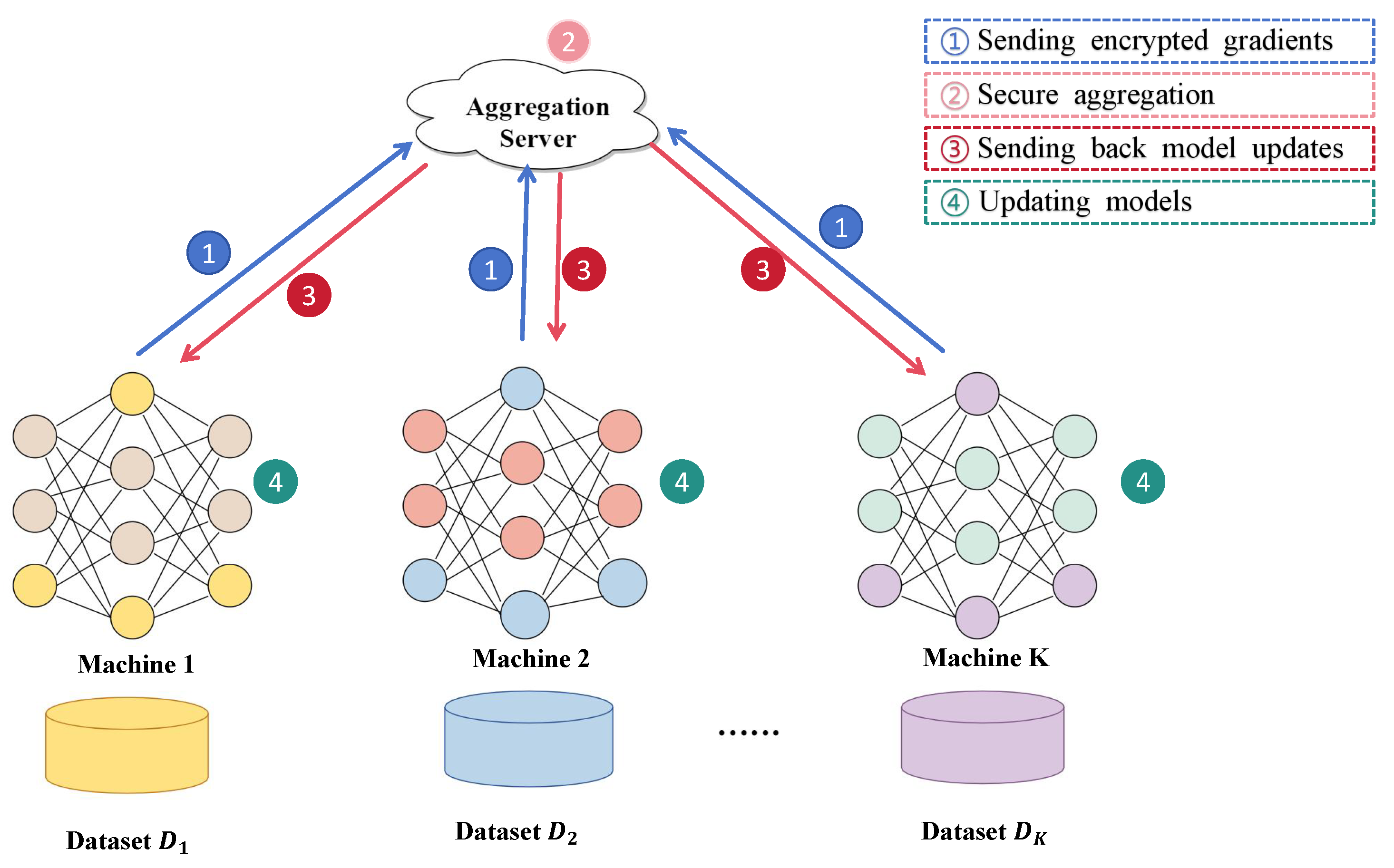
Federated learning is a distributed machine learning framework designed to enable the training of local models using datasets distributed across multiple centers. These locally trained models are then aggregated to collaboratively construct a global model. Throughout the training process, only model parameters are exchanged among the participating centers, while the local datasets $D_i$ remain securely stored at their respective sources. This approach ensures the privacy of local data, enhances data security, and significantly mitigates the risk of privacy breaches. A typical federated learning system is illustrated in Figure 1. In this setup, centers with identical attribute spaces collaborate under the coordination of a parameter aggregation server to optimize and develop a high-performing global model [16].

Within this architecture, the algorithm iteratively processes data until predefined convergence criteria are met, or until the maximum number of iterations or training time is reached.The process of the federated learning algorithm we consider is shown in Algorithm 1.

Algorithm 1 Federated learning algorithm

Input: Server: Initial global model $w_0$, total rounds T

Centers$\left(E\right)$: Local datasets ${\left\{D_i\right\}}_{i=1}^N$, local epochs E

Output: Optimized global model $w_T$

for round $t=0,1,\dots ,T-1$ do

Server executes:

Broadcast current global model $w_t$ to all centers

Centers parallel execute:

Local training:

Initialize local model: $w_{t,0}^i\leftarrow w_t$

for epoch $e=1$ to E do

Split $D_i$ into batches ${\mathcal{B}}_k$ of size B

for each batch ${\mathcal{B}}_k$ do

$w_{t,e}^i\leftarrow w_{t,e-1}^i-\eta \nabla \mathcal{L}(w_{t,e-1}^i;{\mathcal{B}}_k)$

$\mathsf{\Delta }{w}_t^i=w_{t,E}^i-w_t$

Server aggregates:

Receive updates $\{\mathsf{\Delta }{w}_t^i{\}}_{i\in E}$

Compute weighted average:

$w_{t+1}\leftarrow w_t+{\displaystyle \frac{1}{N}}{\sum }_{i\in E}{\displaystyle \frac{|D_i|}{\left|D\right|}}\mathsf{\Delta }{w}_t^i$

end

2.3. Differential Privacy

In this paper, we primarily focus on global differential privacy within the specific context of federated learning. The implementation of the Laplacian mechanism [20] is relatively intricate within this framework, whereas the Gaussian mechanism is considered more suitable due to its advantageous additivity property. We emphasize differential privacy under the Gaussian mechanism. To introduce the mechanism, we first briefly discuss the concept of ($\epsilon$,$\delta$)-approximate differential privacy.

Definition 1

($(\epsilon ,\delta )$-approximate differential privacy). For neighboring datasets that differ in exactly one data record, there exists an algorithm g that its any output $Y(Y\in Range(g\left)\right)$ satisfies the inequality

$$Pr\left[g\left(D\right)=Y\right]\le e^{\epsilon }Pr\left[g\left(D^{\prime }\right)=Y\right]+\delta ;$$

(10)

then the algorithm g satisfies $(\epsilon ,\delta )-$ differential privacy, where $Pr$ denotes the probability of an event occurring, e is the natural base, and ε is a privacy budget.

Approximate differential privacy introduces an additional privacy parameter, $\delta$, compared with strict differential privacy. This parameter controls the failure rate of differential privacy: the smaller the value, the higher the privacy. In general, a smaller value of $\delta$ will be taken to improve the usability of the algorithm under the same privacy protection conditions.

Definition 2

(Gaussian mechanism). The core concept of the Gaussian mechanism is to achieve differential privacy protection by adding a random noise that follows a specific Gaussian distribution to the output result of a function. For a given dataset D and an arbitrary function $g:D\to R^d$, where the $L2-$ global sensitivity of g is $\mathsf{\Delta }g$, the algorithm

$$G\left(D\right)=g\left(D\right)+N(0,{\sigma }^2)$$

(11)

satisfies $(\epsilon ,\delta )-$ differential privacy with $\epsilon <1,\sigma ={\displaystyle \frac{\mathsf{\Delta }g\sqrt{2\ln \left(\frac{1.25}{\delta }\right)}}{\epsilon }}$

3. The Cox-MLP Based on FL with Differential Privacy

We consider the client–server architecture of the federated learning system, whose structure is shown in Figure 1. In such a system, N centers with the same attribute space, with the coordination and assistance of the parameter aggregation server [24], jointly collaborate to optimize the loss

$$l\left(\mathit{\theta }\right)=\sum {\phi }_i{L}_i\left(\mathit{\theta }\right).$$

To ensure the privacy of individual data during the training process, similar to Wei [25], we adopt the differential privacy mechanism when uploading parameters from centers to the server. Specifically, to achieve $(\epsilon ,\delta )$ differential privacy, that is, for neighboring datasets D and $D^{\prime }$ with exactly one different data record, any output result Y ($Y\in Range\left(g\right)$) of the algorithm g satisfies inequality $\mathrm{Pr}[g\left(D\right)=Y]\le e^{\epsilon }\mathrm{Pr}[g\left(D^{\prime }\right)=Y]+\delta$. We need to add noise from the normal distribution $N\left(0,{\sigma }_U^2\right)$ to each parameter. The calculation formula for the standard deviation of the noise is

$${\sigma }_U={\displaystyle \frac{cL\mathsf{\Delta }{g}_U}{\epsilon }},$$

(12)

where c is a constant, and $c\ge \sqrt{2}ln(1.25/\delta )$. L represents the maximum number of exposure times during the process of uploading local parameters to the server, and $\mathsf{\Delta }{g}_U$ is the global sensitivity. If C is the clipping scale of the gradient during the training process in the center, and the minimum value among the data amounts contained in each center is m, then the sensitivity $\mathsf{\Delta }{g}_U={\displaystyle \frac{2c}{m}}$. However, Wei [24] shows that as the times of iterations increases, the risk of privacy leakage will also increase. Therefore, it is necessary to perturb the parameters before the centers upload them, and then the server aggregates the received parameters. In order to maintain the global ($\epsilon ,\delta$)-differential privacy, the server also needs to add Gaussian noise to the parameters according to the training process and then distribute the randomly perturbed parameters to each center. The added noise follows the following normal distribution $N(0,{\sigma }_D^2)$, where the standard deviation ${\sigma }_D$ is calculated according to the global iteration number T and the number of centers participating in the training N as

$${\sigma }_D=\left\{\begin{array}{cc}{\displaystyle \frac{2cC\sqrt{T^2-L^{2}N}}{mN\epsilon }}\hfill & T>L\sqrt{N},\hfill \\ 0\hfill & T\le L\sqrt{N}.\hfill \end{array}\right.$$

(13)

In this manner, the Cox-MLP model demonstrates its superiority in not only fitting complex data relationships better but also protecting data privacy throughout the entire distributed training process. During the training process, the noise added for privacy protection will inevitably affect the performance of the model. To alleviate this problem, we then propose a method based on weight importance to dynamically adjust the magnitude of the noise in differential privacy.

3.1. Adaptive Differential Privacy Based on Layer Sensitivity (LS-ADP)

To balance privacy protection and model performance, in this paper, we propose two methods based on weight importance. The key to the method lies in quantifying the impact of each layer’s weights on the model performance and dynamically adjusting the magnitude of the noise in differential privacy according to this metric.

We consider adopting the idea of random perturbation. Our method evaluates the impact of each weight change on the model’s performance and adjusts the privacy budget allocation strategy dynamically based on this evaluation.

To reduce the computational load, instead of adding random perturbations to each weight $w_{ij}$, we apply the same random noise to all weights in a layer, and add the same random perturbation to all the weights in this layer. Then we calculate the change in the model performance to evaluate the impact of the weight change in this layer. Specifically, after the local training is completed, we first calculate the evaluation index value p of the model without random perturbations as a benchmark. Under the condition that other weights remain unchanged, we add random noise ${\mathbf{x}}_i$ to all the weights ${\mathbf{w}}_i$ in the i-th layer of the model to obtain the weights ${\mathbf{w}}_i^{\prime }$, that is,

$${\mathbf{w}}_i^{\prime }={\mathbf{w}}_i+{\mathbf{x}}_i,$$

$${\mathbf{x}}_i\sim N(0,{\sigma }_U^2\mathbf{I}),$$

$${\sigma }_U={\displaystyle \frac{cL\mathsf{\Delta }{g}_U}{\epsilon }},$$

where ${\mathbf{w}}_i=(w_{i1},w_{i2},\dots ,w_{i{m}_i})$, ${\mathbf{x}}_i=(x_{i1},x_{i2},\dots ,x_{i{m}_i})$, and $m_i$ represents the number of weights in the i-th layer. c is a constant, and $c\ge \sqrt{2}ln(1.25/\delta )$, ensuring that the Gaussian mechanism satisfies $(\epsilon ,\delta )$-DP requirements. L is the maximum times of exposures during the process of uploading local parameters to the server. $\mathsf{\Delta }{g}_U$ is the global sensitivity, $\epsilon$ is the privacy budget, and $\delta$ is the probability of privacy leakage. Through the perturbed model, to re-evaluate the model performance, new evaluation index values $p_i$ ($i=1,2,3,\dots K$) are obtained, where K is the number of layers of weights in the neural network. Calculate the performance change by

$$V_i.={\displaystyle \frac{|p_i-p|}{{\sum }_{i=1}^K|p_i-p|}}$$

(14)

to measure the impact of weight changes in this layer on model performance. The numerator $|p_i-p|$ quantifies the absolute change in performance caused by the perturbation. This value reflects the sensitivity of the model performance to changes in that particular layer. Based on $V_i.$, the privacy budget of weights in the ith layer can be obtained as

$${\epsilon }_i.=\epsilon V_i.,$$

where $\epsilon$ represents the total privacy budget. If $V_i.$ is relatively large, it indicates that even a slight change in the weights of this layer will lead to a significant change on the model performance. Therefore, a larger privacy budget should be allocated to the weights of this layer so that less noise will be added. Conversely, if $V_i.$ is relatively small, it means that the change in the weights of the layer causes a minor impact on the model performance. Thus, a smaller privacy budget is allocated; that is, more noise can be added.

3.2. Random One-Layer Weighted Differential Privacy Algorithm (ROW-DP)

During the training process of neural networks, the gradient descent method is commonly employed to update the weights. Weights that have a significant impact on the model performance usually undergo relatively large changes. Therefore, we take the degree of dispersion of each weight during the local iteration process as an evaluation indicator to assess its importance. Commonly used metrics include variance (Var), standard deviation (Std), range (Range), interquartile range (IQR), and mean absolute error (MAE). Furthermore, some weights may already be near optimal at initialization, exhibiting low dispersion and potentially being underestimated in their contribution to model performance.

To this end, a comprehensive importance measure $V_{ij}$ for the j-th weight ${\mathbf{w}}_{ij}$ of the i-th layer is defined as

$$V_{ij}={\displaystyle \frac{f\left({\mathbf{w}}_{ij}\right)\times \left|w_{ijm}\right|}{\sum \sum f\left({\mathbf{w}}_{ij}\right)\times \left|w_{ijm}\right|}},$$

(15)

where $f\left({\mathbf{w}}_{ij}\right)$ represents the measures of dispersion of the weight ${\mathbf{w}}_{ij}$, which indicates how much the weight fluctuates during the local iterations. ${\mathbf{w}}_{\mathbf{ij}}=(w_{ij1},\dots ,w_{ijm})$, with m denoting the number of local iterations, and $|w_{ijm}|$ is the absolute value of the weight obtained from the last local iteration. Larger magnitudes can contribute more significantly to the model’s predictions. Based on the value of $V_{ij}$, an adaptive privacy budget allocation can be achieved. Specifically, the privacy budget allocated to the weight ${\mathbf{w}}_{ij}$ is

$${\epsilon }_{ij}=\epsilon V_{ij},$$

where $\epsilon$ represents the total privacy budget. If $V_{ij}$ is relatively large, it indicates that the change of ${\mathbf{w}}_{ij}$ has a significant impact on the model performance. Therefore, a larger privacy budget should be allocated to this weight, and less noise should be added. Conversely, a larger privacy budget should be allocated if $V_{ij}$ is relatively small.

When employing the above strategy for privacy protection, if weighted noise is added to the weights of all nodes, excessive noise may be added to the weights of some nodes, resulting in an unstable fitting process. Based on this, we propose a random one weighted layer method (ROW-DP) on top of the original algorithm. That is, the weights of one layer of the neural network are randomly selected to conduct the above adaptive privacy budget allocation, while the same Gaussian-mechanism differential privacy noise is added to the weights of other layers, enabling our algorithm to possess better stability during the training process while increasing randomness. The privacy budget allocation is as

$${\epsilon }_{ij}=\left\{\begin{array}{c}\epsilon {\displaystyle \frac{f\left({\mathbf{w}}_{ij}\right)\times \left|w_{ijm}\right|}{\sum \sum f\left({\mathbf{w}}_{ij}\right)\times \left|w_{ijm}\right|}}, \mathrm{if}{\mathbf{w}}_{ij}\mathrm{in}\mathrm{the}\mathrm{selected}\mathrm{layer}\hfill \\ \epsilon {\displaystyle \frac{1}{M_i}}, \mathrm{if}{\mathbf{w}}_{ij}\mathrm{not}\mathrm{in}\mathrm{the}\mathrm{selected}\mathrm{layer}\hfill \end{array}\right.,$$

(16)

where $M_i$ is the number of weights contained in the layer.

In this way, it can not only effectively protect data privacy but also minimize the impact of privacy protection measures on the model’s predictive performance. This adaptive noise addition strategy can achieve a balance between privacy protection and model utility. The specific steps are as shown in Algorithm 2, as detailed below, with the proofs provided in Appendix A.

Algorithm 2 Adaptive hierarchical differential privacy optimization framework

Input: Server: Initial global model $w_0$, total rounds T

Centers$\left(E\right)$: Local datasets ${\left\{D_i\right\}}_{i=1}^N$,local epochs E

Output: Optimized global model $w_T$

for round $t=0,1,\dots ,T-1$ do

Server executes:

Broadcast current global model $w_t$ to all centers

Centers parallel execute:

Local training:

Initialize local model: ${\mathit{w}}_{\mathit{t},\mathbf{0}}^{\mathit{i}}\leftarrow {\mathit{w}}_{\mathit{t}}$

for epoch $e=1$ to E do

Split $D_i$ into batches ${\mathcal{B}}_k$ of size B

for each batch ${\mathcal{B}}_k$ do

${\mathit{w}}_{\mathit{t},\mathbf{e}}^{\mathit{i}}\leftarrow {\mathit{w}}_{\mathit{t},\mathbf{e}-\mathbf{1}}^{\mathit{i}}-\eta \nabla \mathcal{L}({\mathit{w}}_{\mathit{t},\mathbf{e}-\mathbf{1}}^{\mathit{i}};{\mathcal{B}}_{\mathbf{k}})$

For each weight $w_{tij}$ in the neural network ${\mathit{w}}_{\mathit{t},\mathbf{E}}^{\mathit{i}}$:

Calculate $V_{tij}$ according to (14) or (16).

${\epsilon }_{tij}=\epsilon ·V_{tij}$.

$w_{(t+1)ij}\leftarrow w_{tij}+N(0,{\displaystyle \frac{cL\mathsf{\Delta }{g}_U}{{\epsilon }_{tij}}})$

End

End

Server aggregates:

Receive updates ${\left\{{\mathit{w}}_{\mathit{t}+\mathbf{1}}^{\mathit{i}}\right\}}_{i\in E}$

Compute weighted average:

${\mathit{w}}_{\mathit{t}+\mathbf{1}}\leftarrow {\mathit{w}}_{\mathit{t}}+{\displaystyle \frac{\mathbf{1}}{\mathbf{N}}}{\sum }_{\mathit{i}\in \mathbf{E}}{\displaystyle \frac{|{\mathbf{D}}_{\mathit{i}}|}{\left|\mathbf{D}\right|}}{\mathit{w}}_{\mathit{t}+\mathbf{1}}^{\mathit{i}}$

The noise variance ${\sigma }_2^2$ is calculated by (13), ${\mathit{w}}_{t+1}={\mathit{w}}_{t+1}+N(0,{\sigma }_2^{2}I);$

end

In the next section, we will validate the performance of our algorithm on both simulated and real datasets, comparing it with the NbAFL algorithm. NbAFL assigns equal privacy budgets to each weight before aggregation and broadcasting, without considering the differences between weights. Our algorithm, on the other hand, takes into account the importance of each weight, resulting in better performance in the numerical experiments.

4. Simulation Studies

In this section, we employ simulated data generation to validate the efficacy of our algorithm. We randomly generate the variables $X_1$ and $X_2$ from normal distributions, $X_3$ from a binomial distribution, and $X_4$ from uniform distributions, forming the covariate vector $\mathit{X}={(X_1,X_2,X_3,X_4)}^T$. Subsequently, we sample survival times from the hazard function $h\left(t\right|x)=h_0\left(t\right)exp\left[g\left(x\right)\right]$ and censored times from ${\displaystyle \frac{3}{7}}{h}_0\left(t\right)exp\left[g\left(x\right)\right]$, resulting in data with a 30% censored rate.

For the simulation setup, we assume a baseline hazard function $h_0\left(t\right)=1$ and parameters $\beta =[2.2,5.5,8.8,0]$, with $g\left(x\right)={\beta }^{T}x$. We generate 50,000 data points and partition them into a training set (70%) and a testing set (30%). We allocate average privacy budgets of 0.6, 0.7, 0.8, and 0.9 to the weights. Using centers $N=5$ and global iterations $T=50$, we train our model using both the random one-layer weighted differential privacy (ROW-DP) and the adaptive differential privacy based on layer sensitivity (LS-ADP) algorithms. To assess the performance of our proposed algorithm, we conducted 100 independent experiments and compared the results with the NbAFL algorithm [25]. The NbAFL algorithm ensures privacy protection by assigning an equal privacy budget to each weight during both the upload and broadcast phases. Furthermore, we used the Cox-MLP algorithm [22] without differential privacy (Npdp) as a baseline for comparison.

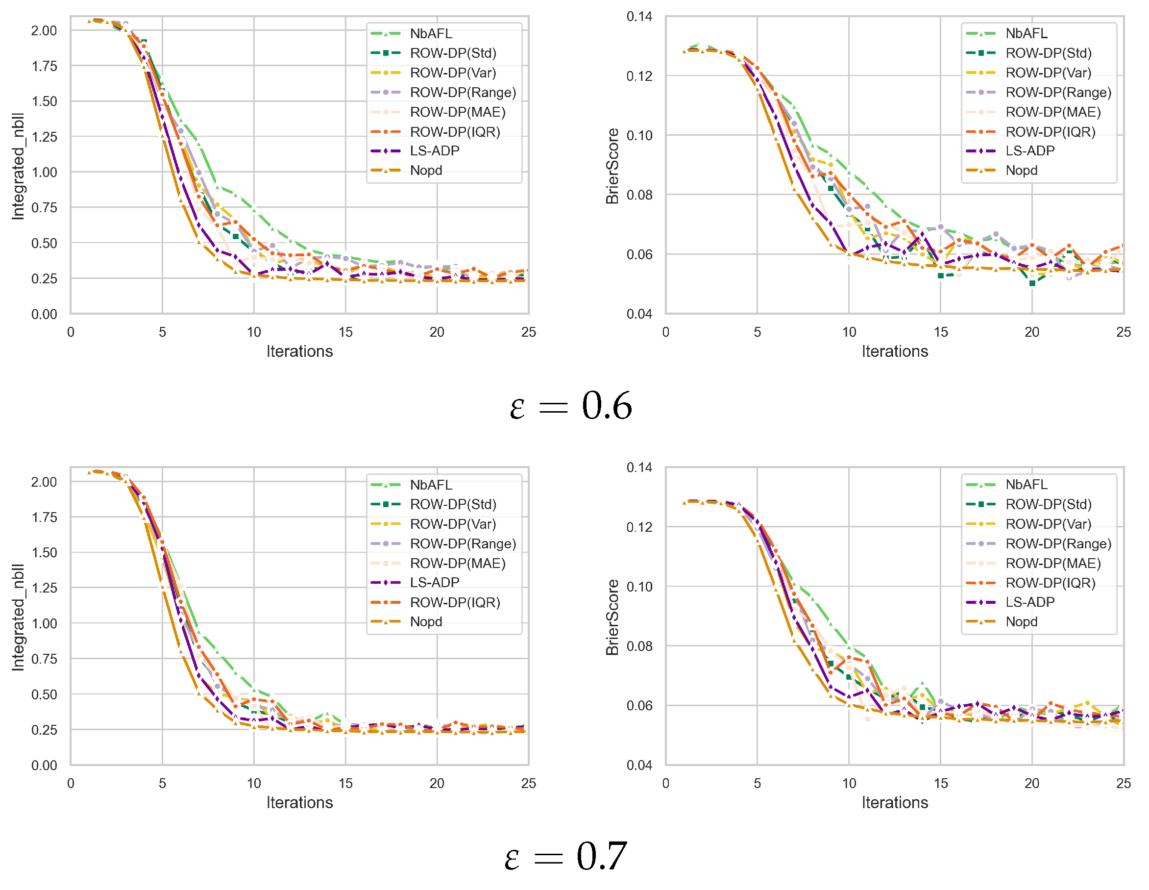
Given the complexities inherent in neural networks, the coefficients associated with each covariate cannot be directly obtained. Therefore, we primarily evaluate our model using the Brier Score and the Integrated Negative Log-Likelihood (INLL). The Brier Score (BS), which ranges from 0 to 1, measures the Mean Squared Error (MSE) between the predicted survival probabilities and the true survival status, with 0 indicating perfect prediction and 1 indicating no predictive value. In survival analysis, for each time point t, the Negative Log-Likelihood gauges the discrepancy between the model’s predicted survival probability and the observed outcome. The Integrated Negative Log-Likelihood, by integrating the Negative Log-Likelihood over all time points, provides a comprehensive evaluation metric, where a lower value implies superior model performance.

Figure 2 and

Table 2. Integrated Negative Log-Likelihood for Cox-MLP (Nopd), LS-ADP, and ROW-DP algorithms under different privacy budgets ($\epsilon$) based on five dispersion measurement methods (Var, Range, Std, MAE, IQR).

Privacy Budget	0.6	0.7	0.8	0.9	1
NbAFL	0.2753	0.2613	0.2581	0.2446	0.2359
ROW-DP(Std)	0.2726	0.2553	0.2541	0.2498	0.2476
ROW-DP(Var)	0.2681	0.2596	0.2572	0.2530	0.2456
ROW-DP(Range)	0.2686	0.2594	0.2567	0.2464	0.2455
ROW-DP(MAE)	0.2692	0.2683	0.2593	0.2515	0.2450
ROW-DP(IQR)	0.2690	0.2600	0.2554	0.2528	0.2365
LS-ADP	0.2560	0.2551	0.2550	0.2464	0.2455
Nopd	0.2309	0.2309	0.2309	0.2309	0.2309

and

Table 3. Brier Score log-likelihood for Cox-MLP(Nopd), LS-ADP, and ROW-DP algorithms under different privacy budgets ($\epsilon$) based on five dispersion measurement methods (Var, Range, Std, MAE, IQR).

Privacy Budget	0.6	0.7	0.8	0.9	1
NbAFL	0.0592	0.0572	0.0549	0.0548	0.0542
ROW-DP(Std)	0.0577	0.0560	0.0553	0.0543	0.0545
ROW-DP(Var)	0.0569	0.0562	0.0555	0.0552	0.0546
ROW-DP(Range)	0.0576	0.0567	0.0553	0.0548	0.0547
ROW-DP(MAE)	0.0561	0.0558	0.0553	0.0548	0.0543
ROW-DP(IQR)	0.0569	0.0569	0.0545	0.0545	0.0544
LS-ADP	0.0551	0.0547	0.0542	0.0543	0.0543
Nopd	0.0540	0.0540	0.0540	0.0540	0.0540

demonstrate that an increase in privacy budget leads to a gradual reduction in noise added during training, and then the influence of differential privacy on models diminishes progressively. Notably, when $\epsilon$ ≥ 0.8, the difference in INLL between ROW-DP/LS-ADP and Nopd narrows to within 0.5%, validating that the impact of DP on model performance becomes negligible at this stage. Under a low privacy budget ($\epsilon$ = 0.6), the LS-ADP method achieves an INLL of 0.2560 and a BS of 0.0551, which are notably superior to NbAFL’s INLL of 0.2753 and BS of 0.0592. This performance advantage is primarily attributable to LS-ADP’s incorporation of weight importance, which enables a more nuanced and refined allocation of the privacy budget. ROW-DP, by employing random single-layer weighting, concentrates noise on layers with lower sensitivity, thereby reducing perturbations to critical parameters. For example, ROW-DP(Var) achieves an INLL of 0.2681 at $\epsilon$ = 0.6, representing a 2.6% (0.2681 vs. 0.2753)) improvement over NbAFL. LS-ADP, which dynamically adjusts noise based on layer sensitivity, further optimizes the allocation of the privacy budget. At $\epsilon$ = 0.6, LS-ADP’s BS is reduced by 3.2% (from 0.0569 to 0.0551) compared with ROW-DP(Var), indicating that its finer control over the distribution of noise provides a distinct advantage. The impact of different dispersion measurement methods on the performance of ROW-DP is significant. For example, at $\epsilon$ = 0.7, ROW-DP(MAE) achieves an INLL of 0.2683, which is 5.196 higher than ROW-DP(Std)(0.2553), indicating that MAE is more sensitive to noise. In contrast, ROW-DP(IQR) achieves an INLL of 0.2365 at $\epsilon$ = 1, which is close to Nopd (0.2309), suggesting that IQR effectively balances noise and model performance under high privacy budgets. This phenomenon suggests that selecting robust dispersion metrics, such as IQR, can further enhance the algorithm’s performance under stringent privacy constraints. Moreover, across all privacy budgets tested, ROW-DP and LS-ADP exhibited performance comparable to or superior to the NbAFL algorithm. Particularly with smaller privacy budgets, when noise levels are higher, ROW-DP and LS-ADP significantly surpass the NbAFL algorithm. This phenomenon can be primarily attributed to an enhanced privacy allocation strategy that mitigates the effects of differential privacy on the performance of the model.

5. A Real Example of LS-ADP and ROW-DP

To validate the utility of our algorithm, we utilize real-world data, the Free Light Chain (FLCHAIN) dataset compiled by T. Therneau et al. The FLCHAIN dataset encompasses 7874 entries, including 9 covariates, as well as survival time and survival status information at the last known contact for each patient. Additionally, 28% of these data points feature censored survival times. Initial data preprocessing includes handling missing covariate values through multiple imputation and subsequent standardization.

To gauge the effectiveness of our algorithm, we employ the C-index, as proposed by Harrell et al. [26]. This index measures the proportion of patient pairs for whom all available predictions align with actual outcomes, indicating the proportion of patients with lower predicted risks who actually exhibit longer survival times. However, the presence of censored data within the dataset can render certain patient pairs ineligible for C-index computation. Specifically, such pairs are deemed unusable and excluded if both patients are censored or if one patient’s censored time precedes the other’s survival time. The C-index ranges from 0 to 1, with 0.5 suggesting model performance equivalent to random guessing, indicating a lack of predictive ability beyond chance. For predictive evaluation, the dataset is randomly divided into an 80% training set and a 20% test set. The average privacy budgets are 3, 4, 5, and 7, and the experiment was conducted 100 times.

Table 4. C-index log-likelihood for Cox-MLP(Nopd), LS-ADP, and ROW-DP algorithms under different privacy budgets ($\epsilon$) based on five dispersion measurement methods (Var, Range, Std, MAE, IQR).

Privacy Budget	3	4	5	7
NbAFL	0.7361	0.7560	0.7656	0.7676
Std	0.7301	0.7484	0.7538	0.7550
Var	0.7292	0.7438	0.7433	0.7573
Range	0.7251	0.7522	0.7530	0.7568
MAE	0.7231	0.7485	0.7515	0.7599
LS-ADP	0.7627	0.7653	0.7678	0.7701
IQR	0.7248	0.7515	0.7585	0.7593
Nopd	0.7701	0.7701	0.7701	0.7701

and Figure 3 demonstrate that the addition of noise in differential privacy diminishes with an increasing privacy budget, which leads to a decreasing influence on model performance and a more stable convergence of the C-index. A comparison of various noise addition methods reveals that, in experiments utilizing instance survival data, the performance discrepancy between the NbAFL and ROW-DP algorithms is negligible. LS-ADP achieves 1.7% higher C-index than NbAFL at $\epsilon =3$ (0.7627 vs. 0.7361), narrowing to 0.3% at $\epsilon =7$ (0.7701 vs. 0.7676). For $\epsilon \ge 5$, all algorithms reach $>98\%$ of Nopd’s performance (0.7701). LS-ADP maintains a $>0.762$ C-index across all $\epsilon$, outperforming ROW-DP variants by 2.1–5.3%. In contrast, the LS-ADP algorithm achieves superior performance, particularly in terms of convergence speed and stability when applied across diverse privacy budgets. Notably, when the privacy budget is low, the advantages of LS-ADP become more pronounced, enabling the accommodation of a higher-performance model while ensuring adequate privacy protection.

6. Conclusions

In this paper, we propose a novel privacy budget allocation mechanism. Relying on the relationship between historical changes in parameters and the model performance, we develop a new federated learning algorithm with differential privacy. The innovation of it lies in achieving adaptive privacy budget allocation based on the relationship between parameter changes and model performance. Our results demonstrate that, while maintaining a fixed total privacy budget, both proposed methods effectively balance the trade-off between global differential privacy protection and global model performance. Notably, under smaller privacy budgets, the ROW-DP and LS-ADP algorithms outperform existing methods, such as NbAFL, which lack well-considered differential privacy budget allocation mechanisms, in metrics such as Integrated Negative Log-Likelihood and Brier Score. Furthermore, LS-ADP demonstrates superior accuracy and stability, making it more suitable for scenarios requiring high model performance. On the other hand, ROW-DP, with its simplicity and lower computational overhead, is better suited for resource-constrained applications. The distinctive characteristics of these two methods offer flexible solutions to meet different practical demands. However, this study does not fully address the adaptability of privacy budget allocation in more complex network structures and in scenarios involving non-independent and identically distributed (Non-IID) data. Currently, the differential privacy protection mechanisms we are discussing are far from sufficient for ensuring privacy protection. Attackers may carry out membership inference attacks, model inversion attacks, attribute inference attacks, data re-identification attacks, and data poisoning attacks. Overall, although research on Cox-MLP differential privacy provides a powerful tool for protecting specific models, in the face of various potential privacy threats, we still need to comprehensively utilize multiple technical means (such as encryption, secure multi-party computation, and access control) to build a more comprehensive and robust data protection system. These limitations will be explored and addressed in future research.

References

- Cox, D.R. Regression Models and Life-Tables. J. R. Stat. Soc. Ser. B Methodol. 1972, 34, 187–220. [Google Scholar] [CrossRef]
- Therneau, T.M.; Grambsch, P.M. Modeling survival data: Extending the Cox model. In Statistics for Biology and Health; Springer: New York, NY, USA, 2000. [Google Scholar]
- Kvamme, H.; Borgan, Ø.; Scheel, I. Time-to-event prediction with neural networks and Cox regression. J. Mach. Learn. Res. 2019, 20, 1–30. [Google Scholar]
- Yin, L.; Feng, J.; Xun, H.; Sun, Z.; Cheng, X. A privacy-preserving federated learning for multiparty data sharing in social IoTs. IEEE Trans. Netw. Sci. Eng. 2021, 8, 2706–2718. [Google Scholar]
- Xu, J.; Glicksberg, B.S.; Su, C.; Walker, P.; Bian, J.; Wang, F. Federated learning for healthcare informatics. J. Healthc. Inform. Res. 2021, 5, 1–19. [Google Scholar] [PubMed]
- Jung, K.; Baek, I.; Kim, S.; Chung, Y.D. LAFD: Local—Differentially Private and Asynchronous Federated Learning with Direct Feedback Alignment. IEEE Access 2023, 11, 86754–86769. [Google Scholar] [CrossRef]
- Khanna, A.; Adams, J.; Antoniades, C.; Bloem, B.R.; Carroll, C.; Cedarbaum, J.; Cosman, J.; Dexter, D.T.; Dockendorf, M.F.; Edgerton, J.; et al. Accelerating Parkinson’s Disease drug development with federated learning approaches. NPJ Park. Dis. 2024, 10, 225. [Google Scholar]
- Bhatia, A.S.; Neira, D.E.B. Federated learning with tensor networks: A quantum AI framework for healthcare. Mach. Learn. Sci. Technol. 2024, 5, 045035. [Google Scholar] [CrossRef]
- Yue, G.; Wei, P.; Zhou, T.; Song, Y.; Zhao, C.; Wang, T.; Lei, B. Specificity-Aware Federated Learning with Dynamic Feature Fusion Network for Imbalanced Medical Image Classification. IEEE J. Biomed. Health Inform. 2024, 28, 6373–6383. [Google Scholar] [CrossRef] [PubMed]
- Zhu, L.; Liu, Z.; Han, S. Deep leakage from gradients. Adv. Neural Inf. Process. Syst. 2019, 32, 1–11. [Google Scholar]
- Geiping, J.; Bauermeister, H.; Dröge, H.; Moeller, M. Inverting gradients-how easy is it to break privacy in federated learning? Adv. Neural Inf. Process. Syst. 2020, 33, 16937–16947. [Google Scholar]
- Bonawitz, K.; Ivanov, V.; Kreuter, B.; Marcedone, A.; McMahan, H.B.; Patel, S.; Ramage, D.; Segal, A.; Seth, K. Practical Secure Aggregation for Privacy-Preserving Machine Learning. In Proceedings of the 2017 ACM SIGSAC Conference on Computer and Communications Security, Dallas, TX, USA, 30 October–3 November 2017; pp. 1132–1147. [Google Scholar]
- Geyer, R.C.; Klein, T.; Nabi, M. Differentially Private Federated Learning: A Client Level Perspective. arXiv 2017, arXiv:1712.07557. [Google Scholar]
- Zhao, C.X.; Sun, Y.; Wang, D.G. Federated learning with Gaussian differential privacy. In Proceedings of the IEEE International Conference on Big Data (Big Data), Atlanta, GA, USA, 10–13 December 2020; pp. 296–301. [Google Scholar]
- Rodríguez-Barroso, N.; Stipcich, G.; Jiménez-López, D.; Ruiz-Millán, J.A.; Martínez-Cámara, E.; González-Seco, G.; Luzón, M.V.; Veganzones, M.A.; Herrera, F. Federated Learning and Differential Privacy: Software tools analysis, the Sherpa.ai FL framework and methodological guidelines for preserving data privacy. Inf. Fusion 2020, 64, 270–292. [Google Scholar] [CrossRef]
- Abadi, M.; Chu, A.; Goodfellow, I.; McMahan, H.B.; Mironov, I.; Talwar, K.; Zhang, L. Deep learning with differential privacy. In Proceedings of the 2016 ACM SIGSAC Conference on Computer and Communications Security, Vienna, Austria, 24–28 October 2016; pp. 308–318. [Google Scholar]
- Dwork, C.; Roth, A. The algorithmic foundations of differential privacy. Found. Trends Theor. Comput. Sci. 2014, 9, 211–407. [Google Scholar] [CrossRef]
- Rieke, N.; Hancox, J.; Li, W.; Milletari, F.; Roth, H.R.; Albarqouni, S.; Bakas, S.; Galtier, M.N.; Landman, B.A.; Maier-Hein, K.; et al. The future of digital health with federated learning. NPJ Digit. Med. 2020, 3, 1–7. [Google Scholar]
- Fu, J.; Chen, Z.; Han, X. Adap DP-FL: Differentially Private Federated Learning with Adaptive Noise. In Proceedings of the 2022 IEEE International Conference on Trust, Security and Privacy in Computing and Communications (TrustCom), Wuhan, China, 9–11 December 2022; pp. 1–6. [Google Scholar]
- Zhao, Z.; Sun, Y.; Bashir, A.K.; Lin, Z. AdaDpFed: A Differentially Private Federated Learning Algorithm with Adaptive Noise on Non-IID Data. IEEE Trans. Consum. Electron. 2024, 70, 2536–2545. [Google Scholar]
- Hu, J.; Wang, Z.; Shen, Y.; Lin, B.; Sun, P.; Pang, X.; Liu, J.; Ren, K. Shield Against Gradient Leakage Attacks: Adaptive Privacy-Preserving Federated Learning. IEEE/ACM Trans. Netw. 2023, 32, 1407–1422. [Google Scholar] [CrossRef]
- Katzman, J.L.; Shaham, U.; Cloninger, A.; Bates, J.; Jiang, T.; Kluger, Y. DeepSurv: Personalized treatment recommender system using a Cox proportional hazards deep neural network. BMC Med. Res. Methodol. 2018, 18, 1–12. [Google Scholar] [CrossRef] [PubMed]
- Klein, J.P.; Moeschberger, M.L. Survival Analysis: Techniques for Censored and Truncated Data, 2nd ed.; Springer: New York, NY, USA, 2003. [Google Scholar]
- Yang, Q.; Liu, Y.; Chen, T.; Tong, Y. Federated machine learning: Concept and applications. ACM Trans. Intell. Syst. Technol. (TIST) 2019, 10, 1–19. [Google Scholar]
- Wei, K.; Li, J.; Ding, M.; Ma, C.; Yang, H.H.; Farokhi, F.; Jin, S.; Quek, T.Q.; Poor, H.V. Federated learning with differential privacy: Algorithms and performance analysis. IEEE Trans. Inf. Forensics Secur. 2020, 15, 3454–3469. [Google Scholar]
- Harrell, F.E.; Lee, K.L.; Mark, D.B. Multivariable prognostic models: Issues in developing models, evaluating assumptions and adequacy, and measuring and reducing errors. Stat. Med. 1996, 15, 361–387. [Google Scholar] [PubMed]
Figure 1.
Client–server architecture.
Figure 2.
Under different privacy budgets ( = 0.6, 0.7, 0.8, 0.9, 1.0), Integrated Negative Log-Likelihood and Brier Score for Cox-MLP (Nopd) algorithm, LS-ADP algorithm, and ROW-DP algorithm based on five discrete degree measurement methods (Var, Range, Std, MAE, IQR).
Figure 3.
Function of C-index of interaction count using seven different colors to represent various privacy budget allocation methods.