Enhancing Wildfire Detection via Trend Estimation Under Auto-Regression Errors

Abstract

In recent years, global weather changes have underscored the importance of wildfire detection, particularly through Uncrewed Aircraft System (UAS)-based smoke detection using Deep Learning (DL) approaches. Among these, object detection algorithms like You Only Look Once version 7 (YOLOv7) have gained significant popularity due to their efficiency in identifying objects within images. However, these algorithms face limitations when applied to video feeds, as they treat each frame as an independent image, failing to track objects across consecutive frames. To address this issue, we propose a parametric Markov Chain Monte Carlo (MCMC) trend estimation algorithm that incorporates an Auto-Regressive ($AR\left(p\right)$) error assumption. We demonstrate that this MCMC algorithm achieves stationarity for the AR(p) model under specific constraints. Additionally, as a parametric method, the proposed algorithm can be applied to any time-related data, enabling the detection of underlying causes of trend changes for further analysis. Finally, we show that the proposed method can “stabilize” YOLOv7 detections, serving as an additional step to enhance the original algorithm’s performance.

1. Introduction

The increasing frequency and intensity of wildfires, exacerbated by climate change, highlight the urgent need for effective detection and management strategies to protect ecosystems, human lives, and economic assets [1]. As wildfires become more unpredictable and widespread, early detection is crucial for minimizing damage and improving response times. However, traditional fire detection methods, such as satellite imaging and ground-based sensors, often suffer from delayed detection, limited coverage, and high operational costs [2].

Recent advancements in image processing, particularly in object detection [3] and image segmentation [4], have significantly improved fire detection accuracy and efficiency. In this context, Uncrewed Aircraft Systems (UASs) have emerged as a promising tool for real-time smoke detection, providing critical support for wildfire prevention and management [5,6]. Unlike conventional methods, UASs can rapidly navigate hazardous environments, offering a flexible and cost-effective solution for monitoring vast and inaccessible areas. By leveraging aerial imagery and sophisticated computer vision algorithms, UAS can detect smoke at its early stages, enabling authorities to respond proactively before fires escalate.

Moreover, by integrating advanced vision-based techniques with artificial intelligence, UASs enable automated smoke detection and tracking in dynamic environments [7]. With their vision-based capabilities, UASs offer significant potential for wildfire surveillance, identification, and management [8]. This approach mitigates both the environmental and social impacts of wildfires, highlighting the critical role of UASs in modern fire management strategies.

A key challenge in vision-based fire detection using video data is the limitation of object detection algorithms. One widely used real-time object detection algorithm is You Only Look Once (YOLO) [9]. Leveraging a Convolutional Neural Network (CNN) architecture, YOLO quickly detects and classifies objects in an image by dividing it into a grid of pixels. YOLOv7 [10] improves upon the original YOLO algorithm by enhancing accuracy and speed through the introduction of Extended Efficient Layer Aggregation Networks (E-ELAN).

While YOLOv7 performs well on static images, its effectiveness declines in video applications. This is because the algorithm processes each video frame independently, disregarding temporal relationships between frames. For instance, due to the temporal dependency of adjacent frames, YOLOv7’s bounding boxes may flicker, leading to inconsistent detections. This can cause errors such as misclassifying clouds as smoke or missing smoke detections in some frames, even when correctly identified in previous ones. To address these limitations, we propose a time-series analysis approach to enhance YOLOv7’s performance by incorporating temporal information, thereby improving the robustness and reliability of UAS-based wildfire detection.

In simple terms, a time series refers to a sequence of variable values recorded at different points in time, such as daily temperature measurements at a weather station [11]. Time series data often exhibits long-term trends, and identifying and extracting these underlying trends can be crucial for better understanding and analysis. Trend extraction is widely used across various fields. For example, the power sector relies on it to forecast daily electricity production [12], while the Department of Transportation uses it to predict state traffic patterns, helping individuals plan their travel more effectively [13].

Trend extraction methods are generally classified into parametric and non-parametric approaches. Classical parametric trend estimation methods, such as Ordinary Least Squares (OLS), include median-of-pairwise slopes regression [14] and segmented regression [15]. The advantage of parametric methods lies in their strong interpretability; when the chosen model accurately represents the underlying data, these methods can achieve high accuracy. However, real-world data often contains unpredictable factors, making it difficult to ensure that a parametric model perfectly fits the data. In such cases, non-parametric trend estimators, such as Hodrick-Prescott (HP) filtering [16] and $l_1$-trend filtering [17], are often preferred.

In this paper, the proposed method falls under the category of parametric trend estimation, as the prescribed fire environment during UAS deployment remains highly consistent. Compared to OLS, the proposed method incorporates additional constraints in the dataset, making it useful not only for stabilizing the YOLOv7 algorithm by predicting smoke instances missed by YOLOv7, but also for identifying key factors influencing smoke trends, such as wind speed, forest type, and UAS movement. The following are the key contributions of this paper:

• Development of a Parametric Trend Estimation Method for Non-Stationary Time Series: We introduce a novel approach to accurately decompose time-series data into its long-term and short-term components, assuming the short-term trend follows an autoregressive ($AR\left(p\right)$) model. This method leverages the inherent autocorrelation in time-series data to identify patterns and similarities between past and present data points, as is commonly observed in such datasets [18].
• Theoretical Justification of the Model: We provide a rigorous theoretical foundation for the proposed parametric estimation method. Under two key assumptions, we demonstrate that the method can be optimized using an MCMC algorithm and that the algorithm converges over successive iterations.
• Application to Wildfire Smoke Detection in Video: The proposed trend estimation method is applied to real-world smoke video data under the Hidden Markov Chain (HMM) structure. Experimental results demonstrate that the method effectively enhances smoke detection by correcting both missed and erroneous detections.

This paper is organized as follows: Section 2 presents some popular trend estimation methods currently in use. Section 3 describes the overall model, assumptions, theoretical support for applying MCMC estimation, and the MCMC algorithm. Section 4 provides two simulation studies to visualize the algorithm’s efficiency. Section 5 compares our model estimation with the YOLOv7 [10] using a wildfire video in the real world. Section 7 shows the future research direction based on the model, and Section 8 summarizes our contribution.

2. Related Works

As mentioned, due to the unpredictable factors when collecting data, popular examples of trending estimation in time series fields are the HP filtering and $l_1$-trend filtering. Compared to HP filtering, $l_1$-trend filtering estimates the trend using a simple linear regression. The benefit of this approach is its interpretability. However, the optimization method for $l_1$-trend filtering is slightly more complicated due to the use of the $l_1$ penalty. A modern solution to this optimization problem is to apply the Markov Chain Monte Carlo (MCMC) process [19]. Without the optimization problem, HP filtering is popular in economics [20]. However, since this method is nonparametric, the model lacks interpretability [21].

Another issue is that both HP filtering and $l_1$ filtering assume that the error terms are independent of time, meaning the time series consists of a single trend function and an error term with constant variance over time (i.e., the error is stationary). However, this stationarity assumption may not be appropriate for analyzing wildfire detection videos, as the motion of wildfire smoke in these videos is influenced by two key time-dependent factors. The first factor is the long-term trend, which is primarily determined by the motion of the UAS capturing the video. The second factor is the short-term trend, which depends on dynamic environmental conditions such as current wind speed, wind direction, wildfire spread, and other contextual variables. This short-term trend introduces a non-stationary error component into the model, making the stationary error assumption inadequate.

In addition to classical HP filtering and $l_1$ filtering, a newer trend estimation method is Singular Spectrum Analysis (SSA) [22,23,24,25]. SSA transforms the time series into a trajectory matrix and applies Principal Component Analysis (PCA) to decompose the matrix into a linear combination of elementary matrices, effectively extracting the latent function. However, similar to HP filtering and l1l1 filtering, SSA also assumes a stationary error term.

To address the issue of non-stationarity, a non-stationary Gaussian process regression model has been proposed [26], which is a non-parametric approach capable of handling time-varying errors. While non-parametric and semi-parametric models excel at making accurate predictions, they face significant limitations in terms of interpretability and facilitating further analysis. These challenges make them less suitable for applications that require a deeper understanding of the underlying processes, such as the dynamics of wildfire smoke or the movement of UAS.

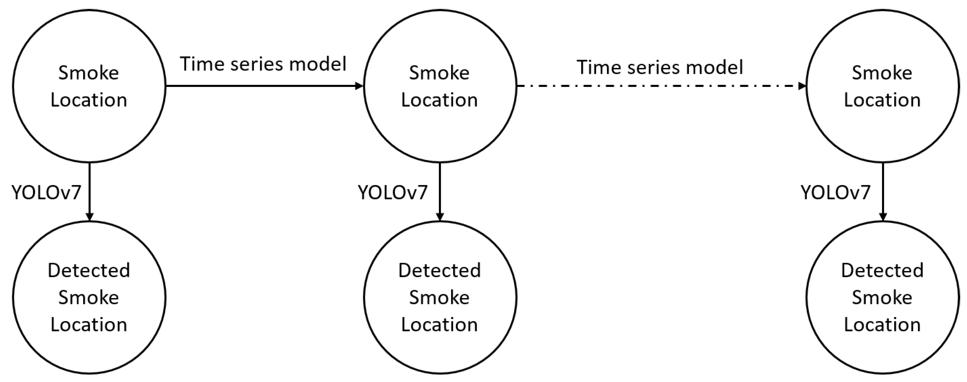
Therefore, we propose a parametric model and combine it with YOLOv7 based on the Hidden Markov Model (HMM) framework, which overcomes these limitations. The proposed method estimates transition probabilities within the HMM using time series data, where the long-term trend is estimated using Ordinary Least Squares (OLS), and the short-term trend is modeled by an $AR\left(p\right)$ process. The emission states correspond to smoke locations identified by the YOLOv7 object detection model (see Figure 1).

This approach allows for the prediction of smoke in frames where YOLOv7 detected it in the previous frame but fails to identify it in the current one. It also corrects false detections and integrates these refined, newly identified frames into the training set, enhancing YOLOv7’s accuracy. Additionally, the trend estimation facilitates further analysis of the factors driving changes in the trend function, providing valuable insights into the dynamics of wildfire smoke.

3. Methodology

In this article, we assume that the location and motion of smoke in a video are governed by two main factors: the long-term trend and the short-term trend. The long-term trend is primarily influenced by the motion of the UAS, while the short-term trend consists of two key components. The first component is the previous smoke location in the video, which ensures temporal continuity and can be predicted using an autoregressive function [27]. The second component includes random factors affecting the smoke, such as wind direction, wind speed, and other environmental variables. Additionally, we assume that these factors are additive, leading to the formulation of the following time-series model.

$$Y\left(t\right)=f\left(t\right)+AR\left(p\right),$$

(1)

where $f\left(t\right)$, a deterministic function, represents the long-term trend, and the short-term trend is modeled by an autoregressive function $AR\left(p\right)$:

$$AR\left(p\right)=Y^{*}\left(t\right)={\alpha }_1{Y}^{*}(t-1)+{\alpha }_2{Y}^{*}(t-2)+\cdots +{\alpha }_p{Y}^{*}(t-p)+{ϵ}_t.$$

(2)

Here, $Y^{*}\left(t\right)=Y\left(t\right)-f\left(t\right)$ represents the deviation of $Y\left(t\right)$ from the trend $f\left(t\right)$, and the error term ${ϵ}_t$ is assumed to be independently and identically distributed (IID) following a distribution with finite mean 0, and variance ${\sigma }^2$ (i.e., ${ϵ}_t\stackrel{iid}{\sim }Dist(0,{\sigma }^2)$). In addition, by the definition of autoregressive function, we have the following assumption.

Assumption 1.

The coefficients ${\alpha }_i$ in Equation (2) satisfy

$$0\le {\alpha }_i\le 1,i=1,2,\dots ,p,\mathit{and}\sum _{i=1}^p{\alpha }_i\le 1.$$

In this setup, we treat $AR\left(p\right)$ as the random error, while the trending function $f\left(t\right)$ is conditionally independent of $AR\left(p\right)$ given

$${\mathbf{Y}}^{*}\left(t\right)={[Y^{*}(t-1),Y^{*}(t-2),\dots ,Y^{*}(t-p)]}^T\in {\mathbb{R}}^p.$$

(3)

Furthermore, by Assumption 1, and leveraging the properties of simple linear regression, we constrain the covariance structure of $Y^{*}\left(t\right)$. That is,

$$\begin{array}{c}\hfill {\displaystyle \frac{Cov[Y^{*}\left(t\right),Y^{*}(t+i)]}{Var\left[Y^{*}\left(t\right)\right]}}\approx {\alpha }_i\in [0,1]\iff 0\le Cov[Y^{*}\left(t\right),Y^{*}(t+i)]\le Var\left[Y^{*}\left(t\right)\right].\end{array}$$

(4)

This ensures that the covariance of is bounded, reflecting the stability of the short-term trend within the time series model.

3.1. Model Assumptions and the Stationary Property

Based on the model assumptions outlined above, we further introduce the following assumption.

Assumption 2.

The initial value of the short-term trend $Y^{*}\left(t\right)$ given by

$$Y^{*}\left(0\right)\sim Dist(0,{\sigma }^2),$$

and for $t\ge 1$, $Y^{*}\left(t\right)$ follows the autoregressive process

$$Y^{*}\left(t\right)=\left\{\begin{array}{cc}{\sum }_{i=1}^t{\alpha }_i{Y}^{*}(t-i)+{ϵ}_t,\hfill & t=1,2,\dots ,p,\hfill \\ AR\left(p\right),\hfill & t>p.\hfill \end{array}\right..$$

(5)

This implies that $Y^{*}\left(t\right)$ is a non-stationary time series with variance changing over time.

With both Assumptions 1 and 2, and given $f\left(t\right)$ and ${\mathbf{Y}}^{*}\left(t\right)$, the conditional expectation of ${\mathbf{Y}}^{*}\left(t\right)$ is

$$E\left[Y\left(t\right)\right|{\mathbf{Y}}^{*}\left(t\right)]=f\left(t\right)+\sum _{i=1}^p{\alpha }_i{Y}^{*}(t-i).$$

(6)

Thus, the long-term trend $f\left(t\right)$ can be expressed as

$$f\left(t\right)=E\left[Y\left(t\right)\right|{\mathbf{Y}}^{*}\left(t\right)]-\sum _{i=1}^p{\alpha }_i{Y}^{*}(t-i),$$

(7)

and the autoregressive component is given by

$$\sum _{i=1}^p{\alpha }_i{Y}^{*}(t-i)=E\left[Y\left(t\right)\right|{\mathbf{Y}}^{*}\left(t\right)]-f\left(t\right),$$

(8)

which is the classical detrending process.

To estimate the trend, we propose the following iterative procedure. Let $Y_{obs}\left(t\right)$ represent the observed time series. The iteration steps are as follows:

• ${\sum }_{i=1}^p{\alpha }_i{Y}^{*}(t-i)=Y_{obs}\left(t\right)-f_i\left(t\right)$.
• $f_{i+1}\left(t\right)=Y_{obs}\left(t\right)-{\sum }_{i=1}^p{\alpha }_i{Y}^{*}(t-i)$.

In this case, the parametric function $f_i\left(t\right)$ is a stationary function that does not change over time, while the error term ${\sum }_{i=1}^p{\alpha }_i{Y}^{*}(t-i)$ is non-stationary, with variance changing over time. Additionally, by taking the variance of both sides of Equation (8), we obtain

$$Var\left[\sum _{i=1}^p{\alpha }_i{Y}^{*}(t-i)\right]=Var\left\{E\left[Y^{*}\left(t\right)\right|{\mathbf{Y}}^{*}\left(t\right)]\right\}\le Var\left[Y^{*}\left(t\right)\right],$$

(9)

where $Var\left[Y^{*}\left(t\right)\right]=Var\left[AR\left(p\right)\right]$. Under these assumptions, we can now state the following theorem.

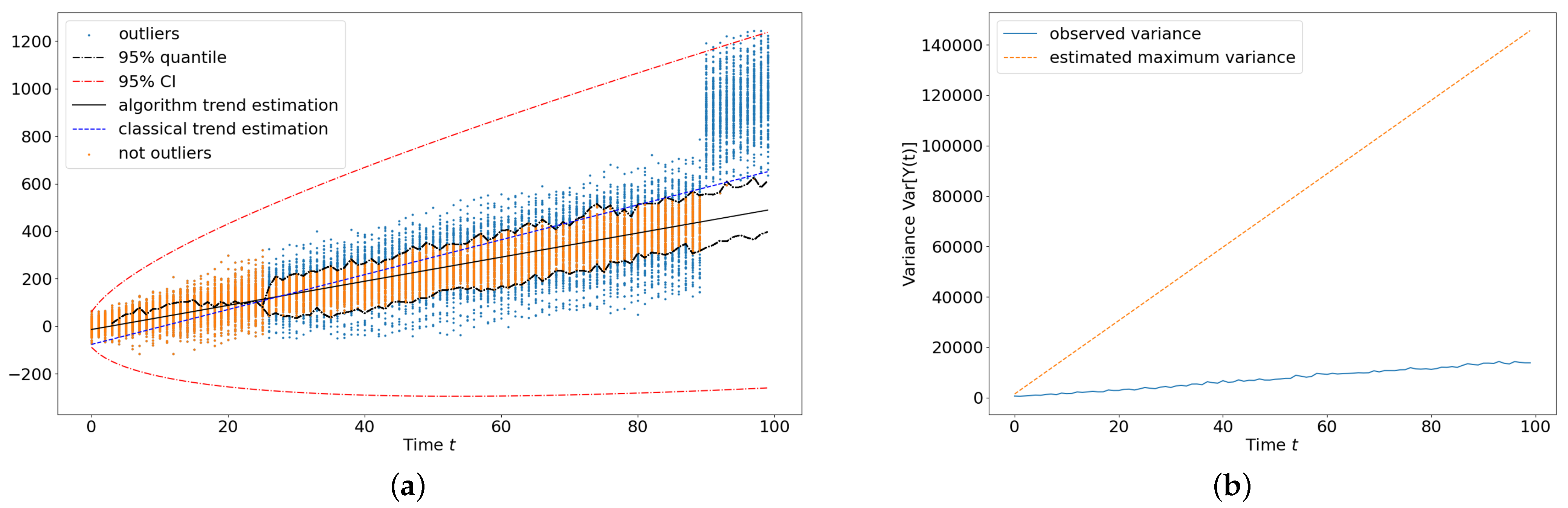
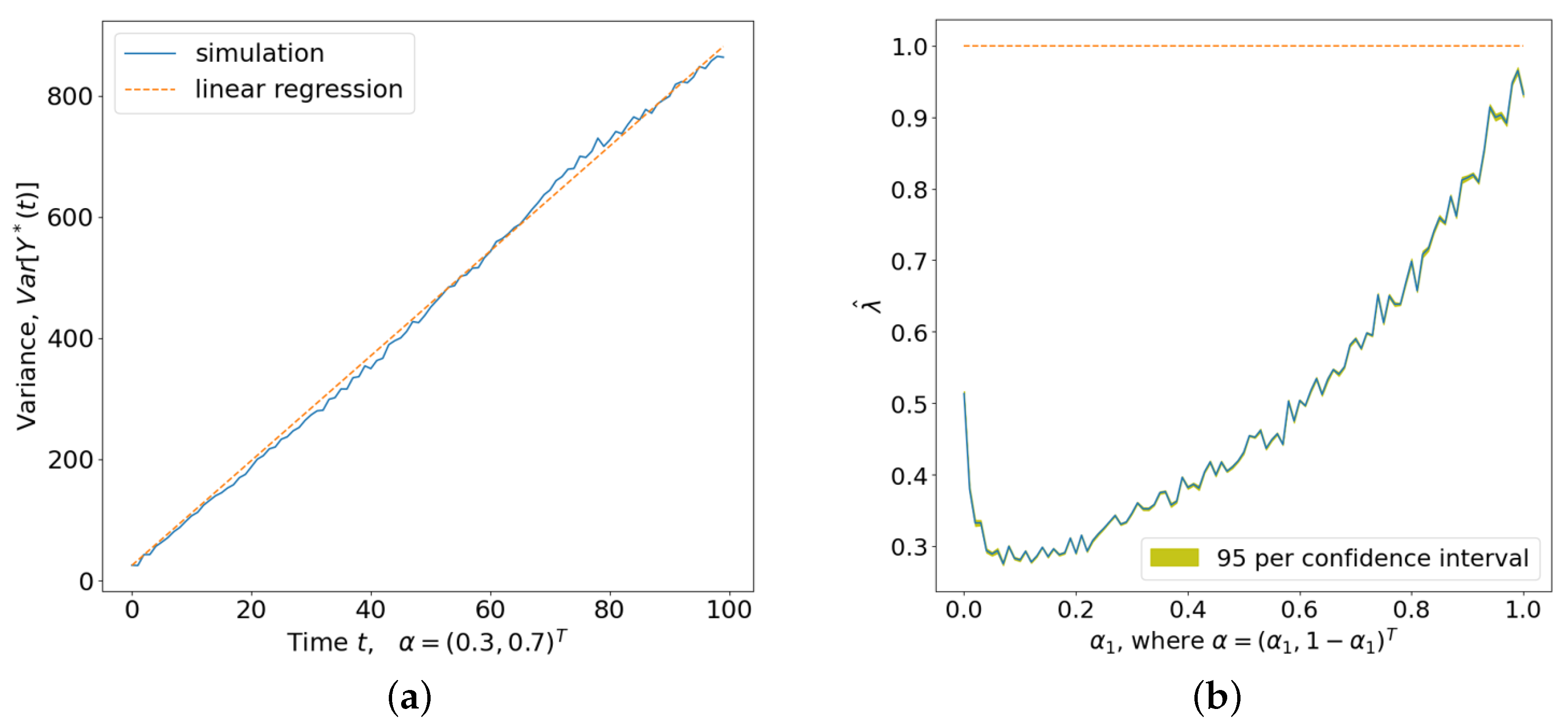
Theorem 1.

Let Assumptions 1 and 2 hold. The variance of $Y^{*}\left(t\right)$ is given by

$$Var\left[Y^{*}\left(t\right)\right]=(1+\lambda t){\sigma }^2,t=1,2,\dots$$

(10)

where $0\le \lambda \le 1$.

With Theorem 1, the proposed method can be applied to non-stationary time series scenarios where variance changes over time. The proof of Theorem 1 is provided in Appendix A, and the empirical conclusions are discussed in the simulation study section. The following inequality follows from Theorem 1.

$$\begin{array}{c}\hfill Var\left[\sum _{i=1}^p{\alpha }_i{Y}^{*}(t-i)\right]\le Var\left[Y^{*}\left(t\right)\right]\le (1+t){\sigma }^2.\end{array}$$

(11)

This inequality implies that the variance of ${\sum }_{i=1}^p{\alpha }_i{Y}^{*}(t-i)$ is finite for a fixed t. Hence, as the iteration of $f\left(t\right)$ progresses, it becomes stationary over extended prediction times t, filtering the non-stationary error terms whose variance changes over time. Therefore, given the form of $f\left(t\right)$, the observed data $Y_{obs}\left(t\right)$, and the prediction horizon t, we can construct an MCMC algorithm to estimate the trending function $f\left(t\right)$.

3.2. The MCMC Algorithm

Algorithm 1 presents the pseudo-code. In our experiment, we set $f\left(t\right)$ as a linear trend since the data collected from the UAS is obtained under consistent motion. However, in theory, this method can also be applied to non-linear cases.

Algorithm 1 MCMC iteration algorithm

1: Initialize the trending function ${\widehat{f}}_0\left(t\right)$.   2: for $i=0,1,\dots ,I-1$ do   3:     Compute $Y^{*}\left(t\right)=Y_{obs}\left(t\right)-f_i\left(t\right)$.   4:     Estimate ${\widehat{AR}}_i\left(p\right)$ given $Y^{*}\left(t\right)$.   5:     Compute $RMS{E}_{AR}$, the rooted mean squared error of ${\widehat{AR}}_i\left(p\right)$, as the estimate of ${\sigma }^2$.   6:     for $j=1,2,\dots ,J$ do   7:         Simulate ${\widehat{Y}}_{ij}^{*}\left(t\right)\sim N({\widehat{AR}}_i\left(p\right),RMS{E}_{AR}^2)$   8:         Estimate ${\widehat{f}}_{i+1,j}\left(t\right)=Y_{obs}\left(t\right)-{\widehat{Y}}_{ij}^{*}\left(t\right)$   9:     Compute the 95% quantile for the $Y\left(t\right)$ estimation. 10:     if $Y_{obs}\left(t\right)\notin ({\widehat{Y}}_{0.025}\left(t\right),{\widehat{Y}}_{0.975}\left(t\right))$ then 11:         set $Y_{obs}\left(t\right)$ as the outlier and remove it from the training data. 12:     Determine ${\widehat{f}}_{i+1}\left(t\right)=Y_{obs}\left(t\right)-{\widehat{Y}}_i^{*}\left(t\right)$, where ${\widehat{Y}}_i^{*}\left(t\right)=Media{n}_j\left({\widehat{Y}}_{ij}^{*}\left(t\right)\right)$. 13: After I iterations, and when kth iteration becomes stationary, where $k<I$, compute the final prediction and the quantile intervals.

This algorithm performs two main tasks. First, it estimates the trending function $f\left(t\right)$. Second, it identifies outliers and non-stationary errors, removes them from the training data, and corrects the trending function $f\left(t\right)$.

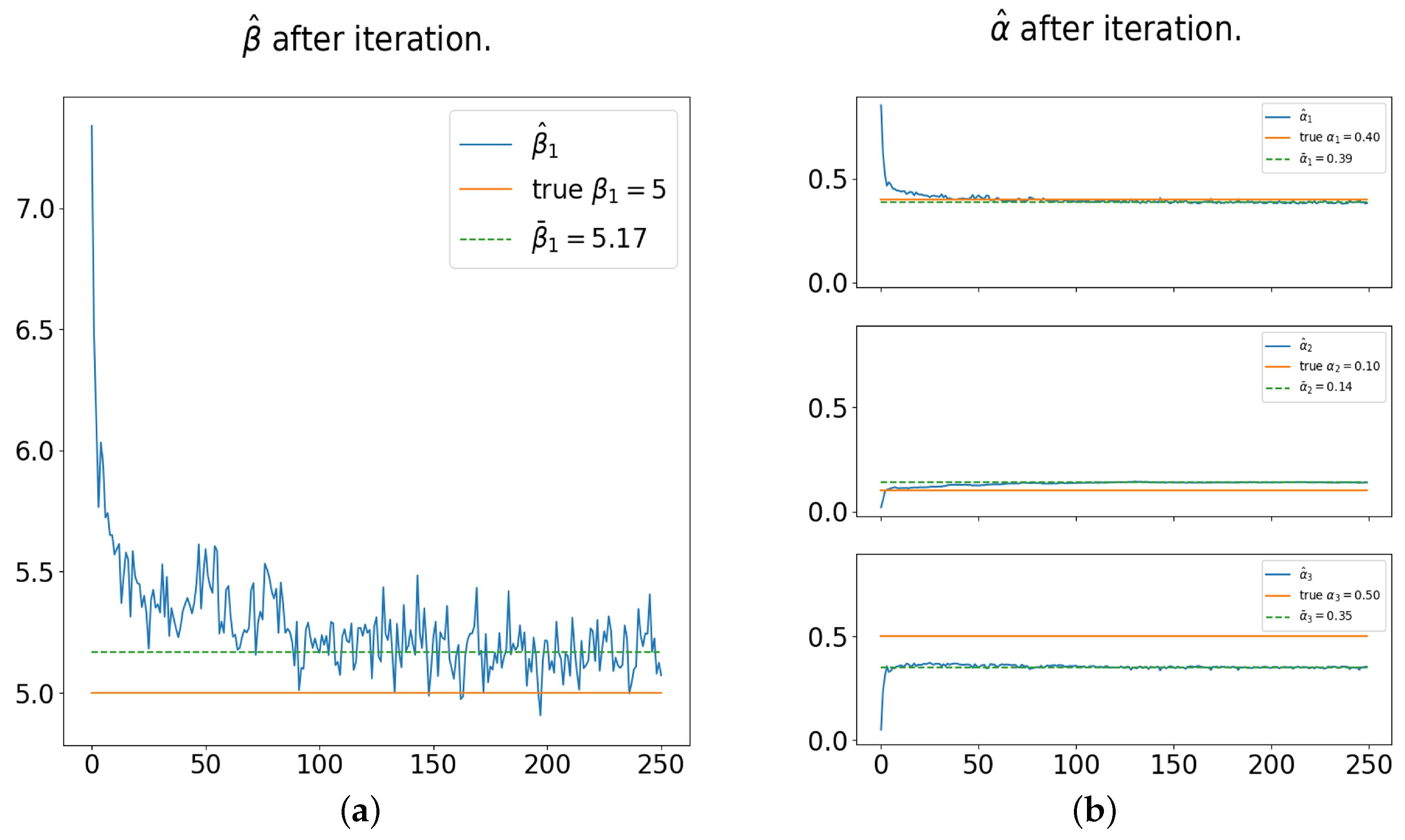
In Line 2 of Algorithm 1, the total number of iterations, I, should be set large enough to ensure the estimated function $\widehat{f}\left(t\right)$ has converged. In our simulation study, the estimates became stationary after 100 iterations. Therefore, empirically, we recommend setting I between 150 and 250 iterations. In Line 6 of Algorithm 1, we set the for-loop parameter $J=50$ since, according to our empirical (i.e., simulation) study, there is no significant difference when $J>50$. In Line 7, we assume ${ϵ}_t$ follows a normal distribution with mean ${\widehat{AR}}_i\left(p\right)$ and standard deviation $RMS{E}_{AR}$, where $RMS{E}_{AR}$ is the root mean squared error (RMSE) of $\widehat{AR}\left(p\right)$ (see Line 5). In Line 12, we use the median to compute ${\widehat{Y}}_i^{*}\left(t\right)$, but it can also be determined by averaging over J iterations of ${\widehat{f}}_{i+1,j}\left(t\right)$. In this paper, the final model is

$$\begin{array}{c}\hfill \widehat{Y}\left(t\right)=\widehat{f}\left(t\right)+\widehat{AR}\left(p\right)=\sum _{i=k}^I{\displaystyle \frac{{\widehat{f}}_i\left(t\right)}{I-k+1}}+\sum _{i=k}^I{\displaystyle \frac{{\widehat{AR}}_{i-1}\left(p\right)}{I-k+1}},\end{array}$$

(12)

where the 95% Percentile Interval is given by the following formula:

$$\begin{array}{cc}\hfill & {\widehat{Y}}_{0.025}\left(t\right)=quantil{e}_i({\widehat{f}}_i\left(t\right)+{\widehat{Y}}_{A{R}_{i-1}}\left(t\right),q=0.025)\hfill \\ \hfill & {\widehat{Y}}_{0.975}\left(t\right)=quantil{e}_i({\widehat{f}}_i\left(t\right)+{\widehat{Y}}_{A{R}_{i-1}}\left(t\right),q=0.975)\hfill \end{array}$$

4. Simulation Study

We construct two simulation studies: one is to simulate the performance of Algorithm 1, and the other is to demonstrate Theorem 1.

4.1. Simulation of $Y\left(t\right)=f\left(t\right)+AR\left(p\right)$

In the simulation study, we let $f\left(t\right)=5t$, a linear trend, and let

$$AR\left(3\right)=0.4Y^{*}(t-1)+0.1Y^{*}(t-2)+0.5Y^{*}(t-3)+ϵ,$$

(13)

where $ϵ\sim N(0,5^2)$. Hence, the simulated data can be expressed as

$$Y\left(t\right)=5t+0.4Y^{*}(t-1)+0.1Y^{*}(t-2)+0.5Y^{*}(t-3)+ϵ.$$

(14)

The simulation contains 150 time series with time length $T=100$ (see Figure 2a). The training data includes the first 25 time points, i.e., $Y\left(0\right),Y\left(1\right),\dots ,Y\left(25\right)$. Notice that we simulate the camera shaking error at time 90. That means the algorithm should be able to split the data into two classes: one is the first 90 time points, and the other one is the last 10 time points.

We apply the Algorithm 1 to the simulation data with iteration $I=250$, and the simulated data $J=50$, the final model is

$$\widehat{Y}\left(t\right)=5.17t+0.39Y^{*}(t-1)+0.14Y^{*}(t-2)+0.35Y^{*}(t-3),$$

(15)

whereas the trend is estimated by simple linear regression (the classical detrending method):

$${\widehat{Y}}^{\prime }\left(t\right)=7.34t+0.85Y^{*}(t-1)+0.02Y^{*}(t-2)+0.05Y^{*}(t-3).$$

(16)

In addition, the standard deviation we estimated is $RMS{E}_{AR}=\widehat{\sigma }\approx 38.16$. Hence, the estimated maximum variance of $Y\left(t\right)$ (see Figure 2b) is

$$\widehat{Var}\left[Y\left(t\right)\right]=(1+t)38.{16}^2.$$

(17)

Table 1. Trending function estimated by classical linear regression vs. the proposed method.

	${\mathit{\beta }}_1$		RMSE
Model	Coef	95% CI or PI	Coef	95% CI or PI
Classical Method	7.34	(7.26, 7.42)	114.34	NA
Proposed Method	5.17	(4.99, 5.38)	145.57	(138.65, 151.60)

shows the estimate and the confidence interval (CI) using linear regression. Because the camera shaking (error) is simulated, the linear regression overestimates the trending effect. On the other hand, the estimate and the percentile interval (PI) using Algorithm 1 show a better result. In addition, the RMSE shows that the simple linear regression (114.34) is overfitting, whereas the RMSE after using Algorithm 1 is not ($145.57$).

Table 2. $AR\left(3\right)$ estimated by the classical detrending method vs. the proposed method.

	${\mathit{\alpha }}_1$		${\mathit{\alpha }}_2$		${\mathit{\alpha }}_3$
Model	Coef	95% CI or PI	Coef	95% CI or PI	Coef	95% CI or PI
Classical Method	0.85	(0.838, 0.870)	0.02	(−0.01, 0.04)	0.05	(0.04, 0.07)
Proposed Method	0.39	(0.38, 0.40)	0.14	(0.139, 0.141)	0.35	(0.34, 0.36)

shows the differences between the classical detrending method and Algorithm 1 for the AR model estimates. The PI of ${\alpha }_1$ estimated by Algorithm 1 includes the true value (0.4), and both ${\alpha }_2$ and ${\alpha }_3$ are close to the true value. However, the classical detrending method using linear regression is not so good.

Figure 2 left visualizes the final result of Algorithm 1 compared with the classical detrending method using linear regression. Notice that, since the camera error, the simple linear regression is not working correctly. Figure 2 right shows the maximum variance estimated and the observed variance. Notice that the maximum variance estimated is the upper bound and always larger than the observed variance.

Figure 3 shows the model estimating iterations by the proposed method. The estimates become stationary after 100 iterations. Hence, the final estimation takes the average of these estimators from 150 to 250 iterations (displayed by the green dashed line).

4.2. Simulation of $Var\left[AR\right(p\left)\right]$

In this simulation, we set

$$Y^{*}\left(t\right)={\alpha }_1{Y}^{*}(t-1)+{\alpha }_2{Y}^{*}(t-2)+ϵ,$$

(18)

where $ϵ\stackrel{iid}{\sim }N(0,5^2)$, and $Y\left(0\right),Y\left(1\right)\stackrel{iid}{\sim }N(0,5^2)$. In addition, we set ${\alpha }_1$ from 0 to 1 by 0.01, and ${\alpha }_2=1-{\alpha }_1$. Moreover, we create 1500 replicates of $Y^{*}\left(0\right),Y^{*}\left(1\right),\dots ,Y^{*}\left(100\right)$, and compute the variance of each time t (i.e., $Var\left[Y^{*}\left(t\right)\right]$, where $t=0,1,\dots ,100$).

After computing $Var\left[Y^{*}\left(t\right)\right]$, we apply simple linear regression to estimate the $\lambda$, that is,

$$Var\left[Y^{*}\left(t\right)\right]={\lambda }^{\prime }t+{\sigma }^2.$$

(19)

Then let $\lambda ={\lambda }^{\prime }/{\sigma }^2$, which leads to the final model

$$Var\left[Y^{*}\left(t\right)\right]=(1+\lambda t){\sigma }^2.$$

(20)

Table 3. Some important $\alpha ={({\alpha }_1,{\alpha }_2)}^T$ simulation results.

	$\mathit{\lambda }$
Important $\mathit{\alpha }$’s	Coef	95% CI
(0, 1)	0.513	(0.510, 0.517)
(0.07, 0.93)	0.275	(0.273, 0.278)
(0.99, 1)	0.965	(0.961, 0.970)
(1, 0)	0.932	(0.928, 0.936)

shows the minimum and the maximum estimates of $\lambda$, and when ${\alpha }_1=1$ is the random walk without drifting (Gaussian process).

Notice that the $\lambda$ estimates’ minimum and maximum are all in the range of $[0,1]$ (see Figure 4b). In addition, Figure 4a visualizes the simulated variance and the linear regression of the variance when ${\alpha }_1=0.3,{\alpha }_2=0.7$.

5. Real-World Data Analysis

5.1. Data Collection

In May 2022, we collaborated with the Tall Timbers Research Station to conduct a controlled burn on their property in Tallahassee, Florida. The burn area, shown in Figure 5a, covers approximately 9 acres of forested land. These controlled burns are routinely performed during the spring to manage weeds and improve soil fertility.

Smoke movement is influenced by various factors, including temperature, external wind, and humidity. While it is mathematically impossible to precisely model all external conditions, our algorithm leverages past smoke movement to summarize these factors as an error term. In other words, our algorithm minimizes the impact of environmental conditions by estimating the trend of the smoke movement and using this trend to predict future movement.

During the burn, we utilized a multirotor UAS to collect data from the event. The UAS’s flight plan initiated from the downwind side, progressing upwind towards the area of active burning. It was operated remotely by a human controller, with sensor data being relayed to a ground station for immediate fire monitoring. Figure 5b shows the flight trajectories captured by the UAS’s onboard GPS, indicating that the drone repeatedly passed over the burn areas to gather environmental information. This operation occurred in the early stages of the controlled burn, just after it was ignited, and lasted for about 15 min before the UAS returned to the ground.

5.2. Data Process and Objective Detection

We utilized YOLOv7, a pre-trained real-time object detection model, to analyze wildfire smoke detection data captured at 30 frames per second by a UAS. YOLOv7, which is based on convolutional neural networks, is renowned for its accuracy in detecting objects in both images and videos. It outputs detailed information, including pixel coordinates of the bounding box center (horizontal x and vertical y), the width and height of the bounding box, confidence scores, and bounding box annotations.

In this dataset, we assume that all accurately detected smoke instances follow the same trend at any given timeframe. Therefore, we average the x-coordinates and y-coordinates of the center points of the bounding boxes provided by YOLOv7 within each frame, resulting in a unique x and y coordinate for each frame. This processed data is then treated as a time series, with the frame ID representing time, to train the proposed model using Algorithm 1. Finally, the trained model is applied to predict future frames, starting with a confirmed bounding box from YOLOv7 as the initial reference point.

Figure 6 shows the PACF of both the x-coordinate and the y-coordinate. According to Figure 6, we use $AR\left(3\right)$ to estimate the random effect. Hence, the model in this data is

$$Y\left(t\right)=f\left(t\right)+AR\left(3\right),$$

(21)

where $f\left(t\right)$ is a linear function determined by different timelines (frame id).

Figure 7 displays a segment of the data (Frames 687–825). In this section, the video captures a single smoke area. However, within a 1 s window (Frames 756–787), the bounding box generated by YOLOv7 fluctuates multiple times due to detection errors, as indicated by the dots in Figure 7. Figure 7a highlights the significant difference between the trend prediction obtained using the classical detrending method (green solid line) and the prediction generated by Algorithm 1 (black dashed line).

The real images on the left in Figure 8 show the YOLOv7 predictions. In Frame 757, as illustrated in Figure 8, YOLOv7 fails to detect the smoke. However, Algorithm 1 successfully identifies the trend and makes an accurate prediction. Therefore, visually, the proposed method appears more “stable” than the original YOLOv7.

6. Results

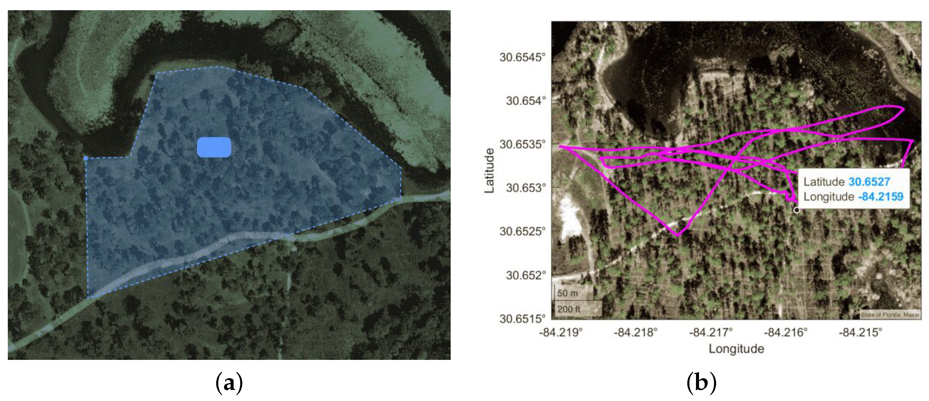
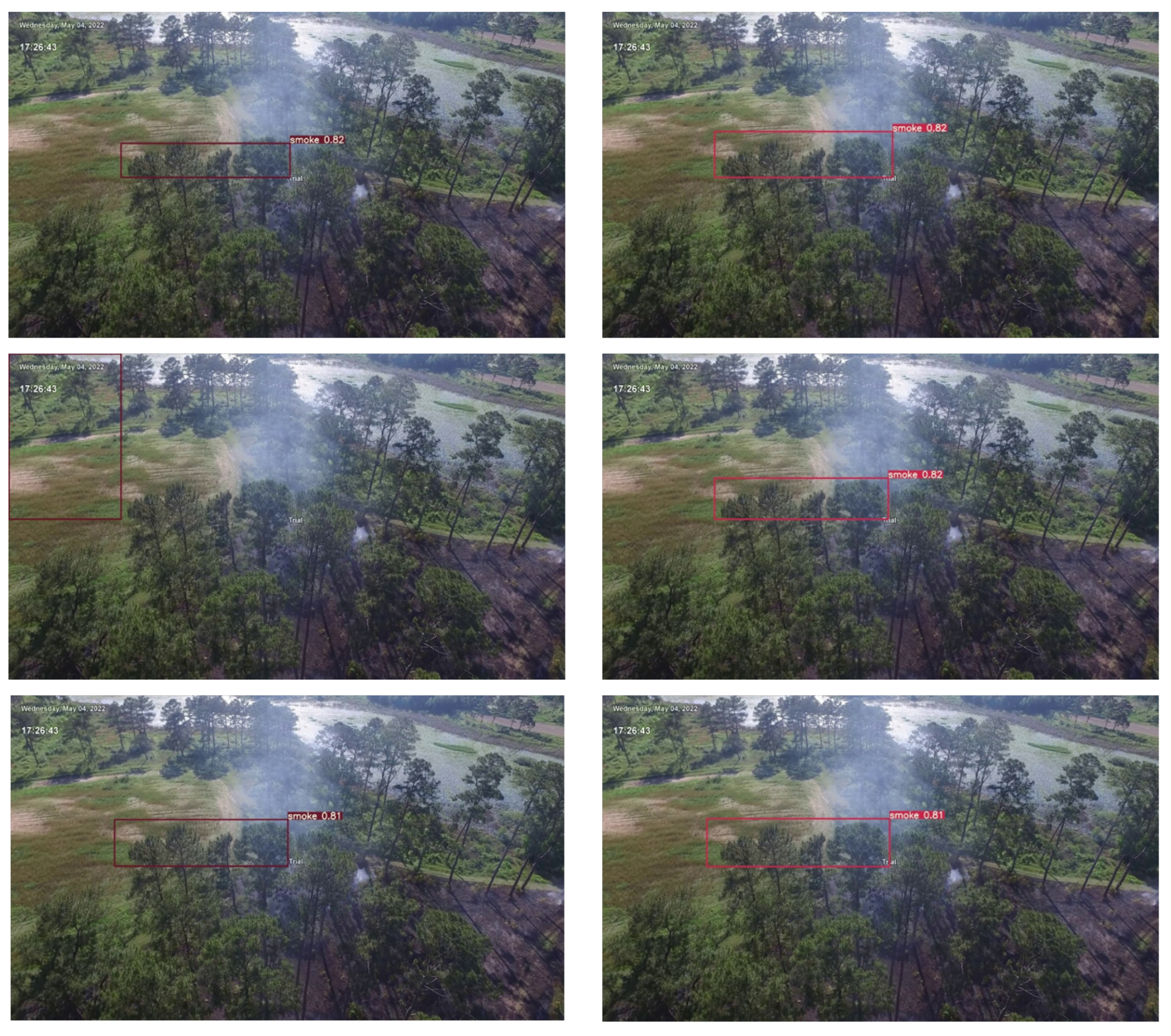
Based on the flight path of the UAS (see Figure 5b), we divide the video frames into three sections. The first section, from Frames 29–500, corresponds to the UAS moving from the forest to the lake, during which YOLOv7 captures most of the smoke and generates the most consistent data. The second section, from Frames 687–825, focuses on the lake, resulting in fewer instances of smoke and less data generated by YOLOv7. In the third section, the UAS returns from the lake to the forest. This section includes both the sky and smoke, causing YOLOv7 to occasionally misidentify clouds as smoke.

Table 4. The trending function of Frame 687–825, estimated by classical linear regression vs. the proposed method.

	${\mathit{\beta }}_1$
Model	Coef	95% CI	RMSE
Classical Method (x-coordinate)	0	(−0.0003, 0.0003)	0.0324
Proposed Method (x-coordinate)	0.0005	(0.0005, 0.0006)	0.0321
Classical Method (y-coordinate)	0.0011	(0.0005, 0.0017)	0.0661
Proposed Method (y-coordinate)	0.0015	(0.0014, 0.0016)	0.0709

presents the numerical results of the trend estimation. For the x-coordinate, there are significant differences between the classical detrending method and Algorithm 1, with our proposed method slightly outperforming the classical approach.

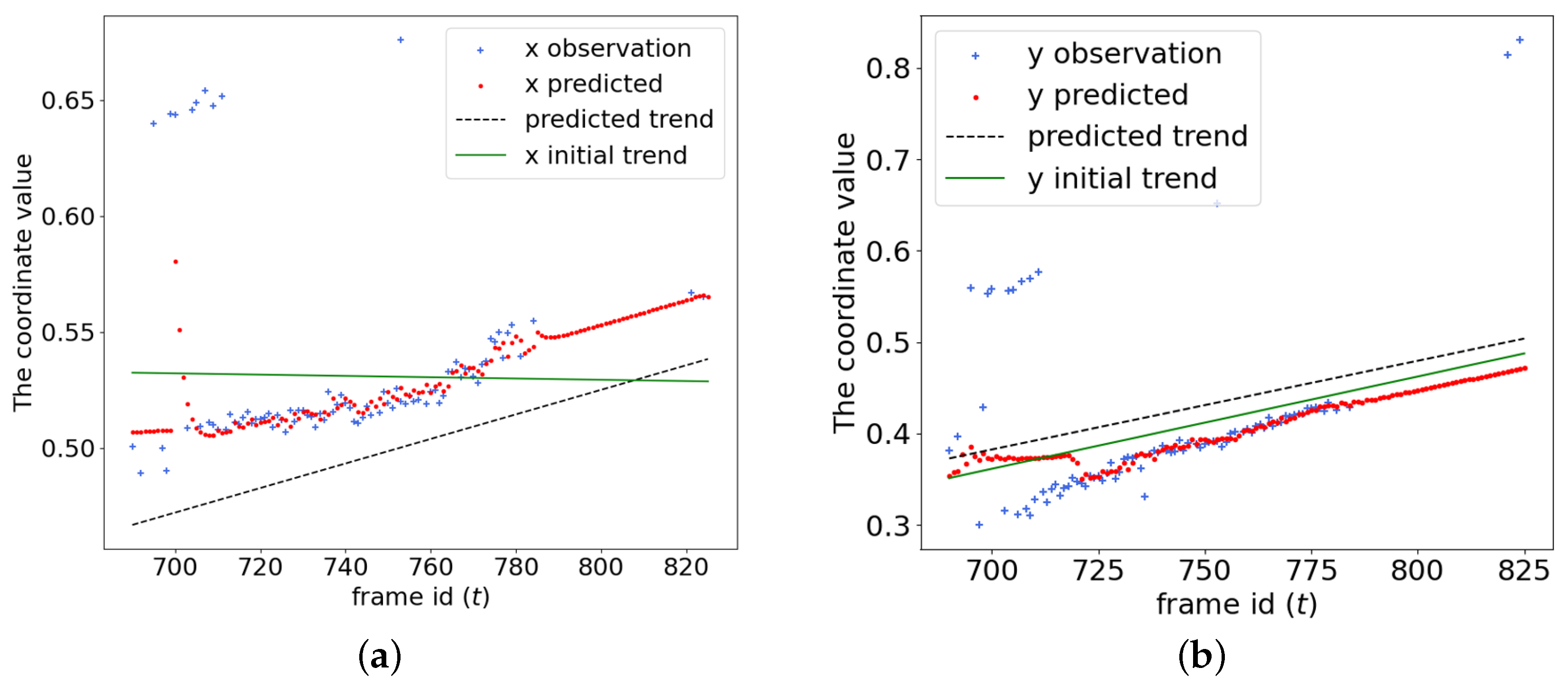
For the y-coordinate, no statistical differences were observed, as the 95% CIs of both the classical method and the proposed method overlap. The outcome is also illustrated in Figure 7b, where the classical method is represented by the green solid line (initial y-trend), and the proposed method is represented by the black dashed line (predicted trend). Additionally, since the classical method treats the points from Frame 687 to 710 as outliers, it adheres more closely to the observed data and, consequently, predicts a different intercept (${\widehat{\beta }}_0$), resulting in a slightly smaller root mean squared error (RMSE).

However, since both methods use only the time-related coefficient (${\widehat{\beta }}_1$) to predict the trend, and the proposed method is ultimately combined with the AR(3) model, discarding the predicted intercepts, the difference between the intercept estimates from both methods is not significant.

Table 5. The $AR\left(3\right)$ of Frames 690–825, estimated by the classical detrending method vs. the proposed method.

	${\mathit{\alpha }}_1$		${\mathit{\alpha }}_2$		${\mathit{\alpha }}_3$
Model	Coef	95% CI	Coef	95% CI	Coef	95% CI
Classical Method (x-coordinate)	0.0464	(−0.1431, 0.2361)	0.0609	(−0.1281, 0.2501)	0.4613	(0.2721, 0.6511)
Proposed Method (x-coordinate)	−0.0129	(−0.1991, 0.1741)	0.0332	(−0.1531, 0.2201)	0.5648	(0.3781, 0.7511)
Classical Method (y-coordinate)	0.2993	(0.0811, 0.5181)	0.0815	(−0.1671, 0.3301)	0.3700	(0.1201, 0.6201)
Proposed Method (y-coordinate)	0.0906	(−0.0991, 0.2801)	0.0428	(−0.1461, 0.2321)	0.5252	(0.3421, 0.7091)

implies that the $AR\left(3\right)$ estimated by both methods has no significant difference except ${\alpha }_1$ in the y-coordinate.

Finally, we apply Algorithm 1 and identify three distinct trending patterns in three frame sections (29–500, 687–825, 3150–3600). The summary result is shown in

Table 6. The trending function estimates using Algorithm 1.

	${\mathit{\beta }}_1$
Frames Section	Coef	95% CI	RMSE
29–500 (x-coordinate)	$1.25\times {10}^{-4}$	($1.20\times {10}^{-4}$, $1.30\times {10}^{-4}$)	0.0808
687–825 (x-coordinate)	$5.29\times {10}^{-4}$	($5.00\times {10}^{-4}$, $6.00\times {10}^{-4}$)	0.0321
3150–3600 (x-coordinate)	$-2.53\times {10}^{-4}$	($-2.68\times {10}^{-4}$, $-2.38\times {10}^{-4}$)	0.0746
29–500 (y-coordinate)	$1.96\times {10}^{-4}$	($1.91\times {10}^{-4}$, $2.00\times {10}^{-4}$)	0.0985
687–825 (y-coordinate)	$1.46\times {10}^{-3}$	($1.37\times {10}^{-3}$, $1.56\times {10}^{-3}$)	0.0709
3150–3600 (y-coordinate)	$2.05\times {10}^{-3}$	($2.00\times {10}^{-3}$, $2.10\times {10}^{-3}$)	0.1213

. The inconsistent RMSE is due to changes in the motion of the observed data. The RMSE between Frames 687 and 825 is the smallest because, during this section, the UAS captured a constant wildfire while maintaining a constant speed. However, between Frames 3150 and 3600, the UAS captured both the wildfire and mistakenly identified some clouds as wildfire, causing the observations to become unstable and resulting in a higher RMSE.

7. Discussion and Future Works

There are two directions to further refine the algorithm in this paper. One is related to segmented regression in the time series. The main problem of segmented regression is determining the number of segments of time (non-identified case) [28]. With Algorithm 1, we can determine if we should make a new segment at time $t+h$ or not by the maximum confidence interval (i.e., $Y(t+h)\pm 1.96\sqrt{(1+h)}\sigma$).

Another direction is to expand the applicability of the algorithm. As mentioned, the current constraint requires the parameters of the autoregressive function to be between 0 and 1, with their sum less than 1. Extending this constraint to the L1 norm, however, may not guarantee a stationary result. Moreover, since the data collected from the UAS is obtained under consistent motion, the algorithm is applied with a linear trend. While the trend function could, in theory, take any form, further studies are needed to explore this possibility. Additionally, in this paper, we employ the HMM-based framework solely to integrate the proposed trend estimation method with YOLOv7, without altering the HMM method itself. Therefore, the proposed approach can be further enhanced by incorporating Bayesian updates to fully leverage the capabilities of the HMM.

8. Conclusions

This paper introduces an MCMC-based trending estimation algorithm that effectively separates long-term and short-term trends for further analysis. In a real-world scenario, we apply this algorithm to wildfire smoke detection data, specifically a 30-frame-per-second video captured by a UAS. Compared to classical detrending methods, our algorithm provides more robust results with this data. Furthermore, the algorithm is used to predict missing data points and correct erroneous detections, ensuring that the bounding box in the video reliably tracks the smoke once detection is confirmed. Additionally, the paper demonstrates that, under certain constraints, the autoregressive function exhibits finite variance that is linearly related to time. As a result, the algorithm becomes stationary when the prediction period is limited.

References

1. Hillayová, M.K.; Holécy, J.; Korísteková, K.; Bakšová, M.; Ostrihoň, M.; Škvarenina, J. Ongoing climatic change increases the risk of wildfires. Case study: Carpathian spruce forests. J. Environ. Manag. 2023, 337, 117620. [Google Scholar] [CrossRef] [PubMed]
2. Hassan, A.; Audu, A. Traditional sensor-based and computer vision-based fire detection systems: A review. Arid Zone J. Eng. Technol. Environ. 2022, 18, 469–492. [Google Scholar]
3. Zaidi, S.S.A.; Ansari, M.S.; Aslam, A.; Kanwal, N.; Asghar, M.; Lee, B. A survey of modern deep learning based object detection models. Digit. Signal Process. 2022, 126, 103514. [Google Scholar] [CrossRef]
4. Minaee, S.; Boykov, Y.; Porikli, F.; Plaza, A.; Kehtarnavaz, N.; Terzopoulos, D. Image segmentation using deep learning: A survey. IEEE Trans. Pattern Anal. Mach. Intell. 2021, 44, 3523–3542. [Google Scholar] [CrossRef]
5. Chen, X.; Hopkins, B.; Wang, H.; O’Neill, L.; Afghah, F.; Razi, A.; Fulé, P.; Coen, J.; Rowell, E.; Watts, A. Wildland Fire Detection and Monitoring Using a Drone-Collected RGB/IR Image Dataset. IEEE Access 2022, 10, 121301–121317. [Google Scholar] [CrossRef]
6. Mukhiddinov, M.; Abdusalomov, A.B.; Cho, J. A Wildfire Smoke Detection System Using Unmanned Aerial Vehicle Images Based on the Optimized YOLOv5. Sensors 2022, 22, 9384. [Google Scholar] [CrossRef]
7. Hossain, F.A.; Zhang, Y.; Yuan, C. A Survey on Forest Fire Monitoring Using Unmanned Aerial Vehicles. In Proceedings of the 2019 3rd International Symposium on Autonomous Systems (ISAS), Shanghai, China, 29–31 May 2019; pp. 484–489. [Google Scholar]
8. Yuan, C.; Zhang, Y.; Liu, Z. A survey on technologies for automatic forest fire monitoring, detection, and fighting using unmanned aerial vehicles and remote sensing techniques. Can. J. For. Res. 2015, 45, 783–792. [Google Scholar] [CrossRef]
9. Redmon, J.; Divvala, S.; Girshick, R.; Farhadi, A. You only look once: Unified, real-time object detection. In Proceedings of the IEEE Conference on Computer Vision and Pattern Recognition (CVPR), Las Vegas, NV, USA, 27–30 June 2016; pp. 779–788. [Google Scholar]
10. Wang, C.Y.; Bochkovskiy, A.; Liao, H.Y.M. YOLOv7: Trainable bag-of-freebies sets new state-of-the-art for real-time object detectors. In Proceedings of the IEEE/CVF Conference on Computer Vision and Pattern Recognition (CVPR), Vancouver, BC, Canada, 17–24 June 2023. [Google Scholar]
11. Houghton, J.T.; Ding, Y.; Griggs, D.J.; Noguer, M.; van der Linden, P.J.; Dai, X.; Maskell, K.; Johnson, C.A. Climate Change 2001: The Scientific Basis; Cambridge University Press: Cambridge, UK, 2001; Volume 881. [Google Scholar]
12. Babu, C.N.; Reddy, B.E. A moving-average filter based hybrid ARIMA–ANN model for forecasting time series data. Appl. Soft Comput. 2014, 23, 27–38. [Google Scholar] [CrossRef]
13. Wang, D.; Luo, H.; Grunder, O.; Lin, Y.; Guo, H. Multi-step ahead electricity price forecasting using a hybrid model based on two-layer decomposition technique and BP neural network optimized by firefly algorithm. Appl. Energy 2017, 190, 390–407. [Google Scholar] [CrossRef]
14. Brinkmann, W. Within-type variability of 700 hPa winter circulation patterns over the Lake Superior basin. Int. J. Climatol. 1999, 19, 41–58. [Google Scholar] [CrossRef]
15. Hamilton, M.; Zhang, Z.; Hariharan, B.; Snavely, N.; Freeman, W.T. Unsupervised semantic segmentation by distilling feature correspondences. arXiv 2022, arXiv:2203.08414. [Google Scholar]
16. Leser, C.E.V. A simple method of trend construction. J. R. Stat. Soc. Ser. B Stat. Methodol. 1961, 23, 91–107. [Google Scholar]
17. Kim, S.J.; Koh, K.; Boyd, S.; Gorinevsky, D. 1 trend filtering. SIAM Rev. 2009, 51, 339–360. [Google Scholar]
18. Xu, W.; Hu, H.; Yang, W. Energy time series forecasting based on empirical mode decomposition and FRBF-AR model. IEEE Access 2019, 7, 36540–36548. [Google Scholar]
19. Heng, Q.; Zhou, H.; Chi, E.C. Bayesian trend filtering via proximal markov chain monte carlo. J. Comput. Graph. Stat. 2023, 32, 938–949. [Google Scholar]
20. Trimbur, T.M. Detrending economic time series: A Bayesian generalization of the Hodrick–Prescott filter. J. Forecast. 2006, 25, 247–273. [Google Scholar]
21. Chen, R.; Xiao, H.; Yang, D. Autoregressive models for matrix-valued time series. J. Econom. 2021, 222, 539–560. [Google Scholar]
22. Vautard, R.; Ghil, M. Singular spectrum analysis in nonlinear dynamics, with applications to paleoclimatic time series. Phys. D Nonlinear Phenom. 1989, 35, 395–424. [Google Scholar] [CrossRef]
23. Broomhead, D.; Jones, R.; King, G.P. Topological dimension and local coordinates from time series data. J. Phys. A Math. Gen. 1987, 20, L563. [Google Scholar]
24. Broomhead, D.S.; King, G.P. Extracting qualitative dynamics from experimental data. Phys. D Nonlinear Phenom. 1986, 20, 217–236. [Google Scholar]
25. Poskitt, D.S. On singular spectrum analysis and stepwise time series reconstruction. J. Time Ser. Anal. 2020, 41, 67–94. [Google Scholar]
26. Paun, I.; Husmeier, D.; Torney, C.J. Stochastic variational inference for scalable non-stationary Gaussian process regression. Stat. Comput. 2023, 33, 44. [Google Scholar]
27. Preisler, H.K.; Schweizer, D.; Cisneros, R.; Procter, T.; Ruminski, M.; Tarnay, L. A statistical model for determining impact of wildland fires on Particulate Matter (PM2.5) in Central California aided by satellite imagery of smoke. Environ. Pollut. 2015, 205, 340–349. [Google Scholar] [CrossRef]
28. Lerman, P. Fitting segmented regression models by grid search. J. R. Stat. Soc. Ser. C Appl. Stat. 1980, 29, 77–84. [Google Scholar]
Figure 1. The Hidden Markov Model assumption by combining our proposed method and the objective detection method (YOLOv7).
Mathematics 13 01046 g001
Figure 2. (a) The blue dashed line is the trending function estimated by the simple method, and the solid black line is the trending function estimated by Algorithm 1. (b) The observed variance (solid blue) and the maximum estimated variance (dashed orange) of Y ( t ) .
Mathematics 13 01046 g002
Figure 3. (a) The trending function estimation (i.e., f ^ ( t ) = β ^ t ) estimated by the proposed method. (b) The A R ( 3 ) function estimation by Algorithm 1. The overall estimation becomes stationary after 100 iterations.
Mathematics 13 01046 g003
Figure 4. (a) V a r [ Y * ( t ) ] vs. t when α = ( 0.3 , 0.7 ) T . (b) The estimates of λ under different α = ( α 1 , 1 α 1 ) T . The red dashed line indicates λ < 1 .
Mathematics 13 01046 g004
Figure 5. (a) The area designated for the controlled burn (outlined in blue). (b) The flight path of the UAS, which is under the control of a human operator. The marked spot on the diagram indicates the starting position.
Mathematics 13 01046 g005
Figure 6. (a) The PACF of the y-coordinate. (b) The PACF of the x-coordinate.
Mathematics 13 01046 g006
Figure 7. (a) The x-coordinate prediction. (b) The y-coordinate prediction.
Mathematics 13 01046 g007
Figure 8. The figures on the left are the YOLOv7 bounding box detection on Frames 756, 757, and 758. The figures on the right are the Algorithm 1 bounding box prediction on Frames 756, 757, and 758.
Mathematics 13 01046 g008