Abstract
In this work, we analyze the vanishing cycles of Feynman loop integrals by the means of the Mayer–Vietoris spectral sequence. A complete classification of possible vanishing geometries is obtained. We use this result for establishing an asymptotic expansion for the loop integrals near their singularity locus and then give explicit formulas for the coefficients of such an expansion. Further development of this framework may potentially lead to exact calculations of one- and two-loop Feynman diagrams, as well as other next-to-leading and higher-order diagrams, in studies of radiative corrections for upcoming lepton–hadron scattering experiments.
Keywords:
algebraic geometry; homology classes; Mayer–Vietoris sequence; pinch map; quantum electrodynamics; Feynman loop integrals; Landau varieties; gamma series; radiative corrections MSC:
14M12; 14M25; 14F10; 14F42; 33C60
1. Introduction
The mathematical study of Feynman integrals has a long history [1,2,3]. In particular, Refs. [2,3] pioneered homological methods, and the use of Picard–Lefschetz theory for Feynman integrals has influenced the development of the theory of hyperfunctions [4]. The book [5] contains reprints of many important papers. The decomposition of the homology of the complement of the union of several hypersurfaces has a long history by itself. Although it is addressed in classical works, it still attracts attention [6] in the context of derived algebraic geometry. The book [7] contains more focused applications of mathematical methods to scattering processes, paying particular attention to the geometry of spaces of momenta as dictated by the combinatorics of Feynman quadrics. Most importantly for our development discussed in the next sections, the use of integration-by-parts (IBP) relations was discussed in [8] (an earlier work is [9]).
In addition to classical work, a major development was initiated in the mathematical literature [10]. This development concerned the use of hypergeometric functions. This approach is very conceptually attractive and has gained a number of followers in the physics literature [11,12,13,14,15,16,17]. An earlier work of one author clarified the relationship to flat bundles. The use of differential equations is the subject of many recent works [18,19]. The analysis of singularities and jumps at the singularities is the subject of modern work [20,21].
Calculations of Feynman loop integrals in particular provide an important test for some modern mathematical methods of quantum field theory and particle physics in general, including relativistic scattering theory. The full non-perturbative theory is a much more complicated problem that incorporates perturbative Feynman integrals as its small part. Therefore, it is essential to develop new mathematical methods that can help achieve detailed understanding of perturbative integrals. Additionally, there is also ample theoretical and phenomenological interest coming from studies of various topics, such as the anomalous magnetic moment of the electron (g-2) [22,23,24,25], two-loop corrections to the Higgs production [26,27,28], and one- and two-loop corrections to lepton–proton [29,30,31,32,33,34,35,36] and lepton–lepton scattering [31,34,37,38,39,40,41,42,43] processes.
There has hitherto been much progress in using algebro-geometric techniques for analyses of Feynman integrals. The topology of contours and its implications have been analyzed in [44,45]. The flat connection in terms of master integrals has been analyzed in a number of cases; see, e.g., [46,47,48,49]. In addition, the connection to modular forms has been explored in [50,51]. The emergence of non-polylogarithmic functions has been studied in [52,53]. There has been a lot of work on this problem in the physics literature [54,55,56,57].
With regard to perturbative integrals, they define a class of functions for external momenta and masses of interacting/scattering physical particles. These are vector functions because multiple integration chains must be considered for them. In fact, they are sections of a flat vector bundle, the pullback of the Gauss–Manin connection to the physical locus. Such functions have regular singularities along Landau varieties and are also the pullback of the solutions to the holonomic GZK D-module [58]. Pullback here is meant in the sense of the theory of holonomic D-modules [59,60]. Such pullback can be taken on a singular set in the parameter space. It is known that physical spaces correspond to a deep stratum in the space of generic kinematic invariants [12,61]. The general theory of such pullbacks involves the theory of b-functions [62]. For a general reference on holonomic D-modules and associated Gauss–Manin connections, see [60,63,64]. For the role of Landau varieties in the analysis of integrals of the hypergeometric type (in particular, from the point of view of underlying meromorphic connection), see [65,66].
Although a large body of general mathematical knowledge has been accumulated about the aforementioned objects [59,65,67], some elementary questions about them remain unaddressed. For example, first-order equations, which those functions satisfy to, are still missing, such that these equations might be consistent with the symmetry of Feynman diagrams. While there has been a lot of research about differential equations’ methods (emerging as dominant methods of computation) [13,54], there is no closed-form expression for those equations. This is especially true for first-order equations, or the Pfaffian form [60]. Given this, such equations could be very important for the numerical evaluation of Feynman loop integrals. Their state of the art can be assessed by focusing on the family of propagator-type diagrams [47,50,68]. For the evaluation of the loop integrals, one must start with an analysis of their behavior near singularities. Although particular cases, such as double-logarithmic asymptotic analysis, are well known, the general case has not been treated in the literature. Furthermore, the exponents of asymptotic expansion near the singularities should provide information about the diagonal part of the flat connection, when it is restricted to the singularity locus. Information on the connection matrices is very limited.
Just as a summary, the study of singularities of perturbative Feynman loop integrals is an important subject, and from a mathematical point of view, Feynman integrals are examples of integrals of rational functions with parameters. The theory of their singularities is very complex, and most results, including those of this work, focus on special cases. In particular, our paper focuses on an asymptotic analysis of perturbative loop integrals near their singularities, with some essential applications discussed in the paper. The structure of this paper is organized as follows.
- (Section 2) We start the analysis in the momentum q-space.
- (Section 3) Then, we continue with a discussion of vanishing cycles since they are a mechanism that leads to the formation of singularities. One can observe the usefulness of the Mayer–Vietoris spectral sequence for a classification of possible types of singularities (for a general introduction to the use of Mayer–Vietoris sequences as applied to the topology of projective complete intersections, we refer to Refs. [69,70]). We give a complete classification of the localization of the vanishing cycles with the case of generic polynomials. Non-local vanishing cycles are outlined as well.
- (Section 4) Herein, we introduce the so-called “pinch map”: a map from the singular locus to the space of the (virtual) loop momenta of particles that gives the location of a point to which the vanishing cycle becomes contractible. The pinch map simplifies calculations for asymptotic analysis and must have some meaning for generic GZK functions as well. Two cases of pinching are presented: with general polynomials and with Feynman loop integrals.
- (Section 5) We consider specific examples of vertex loop diagrams, which may potentially be applied to the lepton–proton () scattering process (the scattering of spin-1/2 particles).
- (Section 6) The so-called “-series” method is outlined, through which it may be possible to later calculate the scattering amplitudes and cross-sections with lowest- and higher-order radiative corrections of QED (quantum electrodynamics), by computing the contributions from one-loop and two-loop Feynman diagrams, as well as from other next-to-leading and higher-order diagrams.
- (Section 7) At the end, we discuss our results and give a direction for future developments.
2. Preliminaries
We start by considering Feynman-type scalar integrals given by
where is the particle propagator, with the momentum , the mass , and
where is the loop momentum and is an integer-valued matrix (see notation in [71]).
Throughout this paper, we consider dimensionally regulated integrals such that
where d is the number of dimensions and L is the number of loops. One should understand as . Analytic continuation in the dimensions is performed in the usual way: the symbol for the dimension is kept free and the resulting analytic functions, such as Gamma factors, are treated as functions of the complex d.
It is convenient to compactify the space of loop momenta to the projective space by adding the boundary . The original integration chain is , which is a real projective space class. While the original integration is performed over the Euclidean space , the correct homological interpretation in terms of homology classes requires passing to compactification and treating the original integration chain as representing a relative homology class. This is the precise homological meaning of “integrating from minus infinity to plus infinity”. Analytic continuation is achieved by moving the chain along with the analytic continuation path. Expressed with some more detail, the analytic continuation is performed by varying the chain representative of the homology class along the path of that continuation. Then, singularities develop through this path such that it is impossible to choose a homologous contour differing from the original one by a chain of homologies. This is the basic vanishing cycle mechanism, which we shall exploit in this paper.
3. Homology Vanishing Cycles
3.1. Vanishing Cycles and Generic Polynomials
This section discusses the choice of contour of integration in the integral of Formula (1). The original integral has prescription. This precisely amounts to the possibility of moving the integration chain away from the zero set of the Feynman quadrics. Then, we have the following:
In this formula, is the intersection of the zero set of the Feynman quadrics with the hyperplane . In our dimensional regularization scheme, we analytically continue to these ds (dimensions), such that the integrand has no pole in the infinitely remote hyperplane. This amounts to the usual power-counting argument.
There is a cycle in even dimensions in the homology group of (where, for convenience, we put and ). This cycle does not change under monodromy, and monodromy generates cycles that are in the image of the tube map (the tube maps are explained in [72]). By using the Alexander duality (tube mapping), we can reduce the computation of these cycles to
where the integration chain is given in a different homology group. Note that the Alexander duality and its use in topology of projective varieties is explained [73,74]. Tube mapping can be defined for singular varieties. In this case, the fiber over points in the singular set is the intersection of the normal cone with a sphere of small diameter.
The variety has multiple irreducible components; therefore, the use of the Mayer–Vietoris spectral sequence is appropriate in this case. The Mayer–Vietoris exact sequence can be applied to the tubular neighborhood of the (in general, singular) variety . It reduces the entire computation to
where I is the propagator tuples, , a multi-index in the subscript of the homology group of . Formula (6) gives a domain, where the vanishing cycles lie (in momentum space representation).
The above Mayer–Vietoris spectral sequence of is applicable to more general integrals, such as
where we integrate the rational form of the type and / are different polynomials but of a generic type. denotes the complex conjugation of . For definiteness, we focus on the integral of the type
Polynomials of the type are used only in generalized integrals, like in (7). Based on (8), the Mayer–Vietoris sequence allows us to reduce the homology computation to the computation of
In this case, there is more information to utilize. We are actually interested in the image of
in under the de Rham isomorphism, where is the Dolbeault cohomology (see Refs. [75,76] for a discussion of the de Rham vs. Dolbeault cohomology in the context of Feynman integrals). By in the above, we mean the image Dolbeault cohomology in the cohomology with integer coefficients. Consequently, we are particularly interested in the part of cohomology of this specific type. Additionally, there is a dual Mayer–Vietoris sequence that can be made to obtain the Hodge filtrations [77,78,79].
3.2. Non-Local Vanishing Cycles
In this section, we analyze non-local vanishing cycles in the context of [80]. And these singularities are quite distinct from the ones considered in [81].
There are strata in the parameter space of the polynomials , which correspond to non-local vanishing cycles. These strata can be approached by curves lying strictly inside the complement of the discriminant of P. Such strata are largely beyond discussion in the literature. For instance, they are not covered in [65,82]; nevertheless, there is some discussion in [83]. Here, we only remark that such non-local vanishing in principle admits combinatorial classification in terms of the following:
- (i)
- The number of derivatives, , that vanish along the stratum for some set of multi-indices, ;
- (ii)
- The geometric locus, where such vanishing happens.
If the geometric locus of the vanishing is given, i.e., the locus of q, in which the vanishing takes place, e.g., in terms of parameterization, then finding equations for the locus in the parameter space ( here and in the following denotes a typical multi-index, ) becomes relatively straightforward by applying the elimination techniques based on the Grobner bases. If only the type of singularity is known, then it becomes a modulus problem, and general GIT (geometric invariant theory) techniques are necessary [84]. By type, we mean scheme-theoretic data that include the dimensionality of the components, their own singularities (in terms of the degeneration of the tangent bundle), and the intersection theory of components.
GIT techniques are very useful in the analysis of bundles that we consider because these bundles typically possess a large degree of symmetry, in particular toric symmetry. The precise characterization of these bundles is only possible after the techniques of GIT are extended sufficiently, such that they can be used in treating Koszul complexes resulting from integration by parts [10], as well as in the conversion from D-modules to corresponding flat connections. This subject is far reaching, since it, e.g., includes a discussion of bases analogous to the polylogarithm bases for the arbitrary divisor’s case and for the bundles with logarithmic singularities for its complement. Some discussion of these topics is available in [74]. It is intimately tied with various categories of modules associated with the components of the divisor.
4. Introduction of Pinch Map
4.1. Pinch Map I: General Polynomials
For the generic stratum of the discriminant locus, the vanishing occurs at some point. In fact, for the generic stratum of the GZK discriminant, the pinching is quadratic. For higher-order isolated singularities of the type treated in Milnor’s classic [85], the vanishing is also local, though it is, in general, non-quadratic [65,86].
Theorem 1.
For the generic stratum of the GZK discriminant for a polynomial, , the vanishing cycles become contractibe to the point
where are rational functions defined everywhere on the main stratum of the GZK discriminant ( must not be confused with , where the latter is just a local symbol for a generic polynomial, while the former is actually the solution for a pinch point). If the vanishing is still local (i.e., the solution of the degeneracy equations consists of isolated points), then the vanishing locus is given by the restriction of the above map to a substratum of the discriminant. The equation for this stratum is obtained by the elimination of from
for a given set of α.
Proof.
The proof can be obtained by the adaptation of the standard Sylvester techniques [10]. In this regard, the question of practical importance is whether an explicit expression for in terms of the GZK discriminants can be obtained, which is a much more challenging task [87,88]. It involves notions that generalize discriminants of exact sequences (the so-called Whitehead torsion [89,90]) to the case of spectral sequences. In fact, the toric nature of the problem can be used for imposing further combinatorial symmetry on the problem. It includes generalizing the notion of the spectral sequence for the case of multiple gradings (giving rise to multidimensional sheets between which the differentials act) and for the needs of combinatorial elimination theory, going beyond the scope of this paper. □
4.2. Pinch Map II: Feynman Loop Integrals
Feynman loop integrals present a highly degenerate case for vanishing cycles’ analysis. Indeed, each of the integral quadrics has a singularity locus (where the derivative vanishes identically) of the dimension . Nonetheless, there is a remnant of the locality of pinching, as we demonstrate in this section. The key observation stems from the use of the Mayer–Vietoris spectral sequence. We observe that for each vanishing cycle, in every , there is a group of propagators , such that there is a vanishing cycle in . For simplicity, we focus here on the vanishing cycles at the finite distance of the momentum space, , rather than of the boundary at infinity. This latter case can be analyzed analogously.
In the following theorem, we analyze the case when the vanishing cycle occurs in the loop momenta . These loop momenta are fixed by the pinch condition. The rest of the loop momenta are not fixed and integration is performed over these coordinates.
Theorem 2.
Vanishing cycles at a finite distance are completely classified by the tuples, , of the propagators, such that there is degeneracy among the tangent cones to the varieties . Such vanishing cycles are contractible to a (pinch) point:
which is a rational function of the masses and external momenta of interacting (scattering) physical particles. The rest of the internal (virtual) loop momenta is arbitrary.
Proof.
The proof follows from the fact that the degeneracy among tangents to can be written as
This set of equations with the factors , where each defines a point in a projective space of the corresponding dimension (not all s are zero), can be solved with
where there can be linear relations among . These coefficients are removed from the system of due to the homogeneity requirement. □
It is convenient to introduce a somewhat more general family of integrals as follows:
We analyze asymptotic expansion near the Morse-type pinch point at . We assume that there is a vanishing cycle in the system, , and the rest of the polynomials do not vanish at 0. Then, we can write
where is a small parameter that can be thought of as the value of the corresponding Landau polynomial. corresponds to the vanishing cycle contracting to the point. We split , such that
and spans the space dual to for some integer, m. is at least quadratic in .
We study the asymptotic expansion of the integral
near the stratum in the parameter space, where there is a Morse singularity in the intersection , which we assume to be a complete intersection at generic values of parameters.
Theorem 3.
There is the following asymptotic expansion near the regular singularity :
where R is a regular function near generic points of the discriminantal locus (it can have singularities along substrata), and
and
The numbers are the coefficients of the linear terms in (17). The momenta forming the set I in the polynomials must be evaluated at the pinch point 0.
In this theorem, k polynomials, , define the pinch point. The asymptotic expansion occurs in the last polynomial, , evaluated at the pinch point. In symmetric notation, we express this using a determinant.
Proof.
We will prove a slightly more general result. Let us consider the integral
where is some regular function and
for which we are interested in an asymptotic expansion near , where and are one- and two-variable polynomial functions. By using a local change in variables,
one can transform the integral in (21) to the form of
where the symbol denotes the polynomial with the lowest index. We do not preserve the symmetry between polynomials and choose one of them. In the end, the expressions should be symmetric with respect to permutation of polynomials, and this is an additional check of our calculation. From here, we see that the contour can be deformed into an elementary loop around (the original contour is the long contour corresponding to the vanishing cycle). □
The following lemma is standard.
Lemma 1.
We have an asymptotic expansion:
where ξ and η are of the same order of magnitude. Here, it is assumed that the contour passes between and .
Lemma 2.
We have an asymptotic expansion for a generic quadratic form :
in which are regular functions of ϵ and at , is the volume of the unit sphere of the dimension , and Q is a nondegenerate quadratic form.
Then, Theorem 3 follows from the above two lemmas. We can also simplify the statement of the theorem to the following form:
where is a function of , is the coordinates on the manifold , and is a contour of integration. If (the number of loops), then the coefficients are algebraic functions. In general, they involve integration over other loop momenta. In the next section, we write an example of such an function involving integration over other loop momenta.
Remark 1.
The term in (20) contains terms that are of a higher order in ϵ and . The branching behavior of the integral comes from the region of momenta, where . The proof of the theorem essentially states that if a vanishing cycle is formed by transversely intersecting k hypersurfaces, then it is possible to deform the contour of integration in a way that one can take the residue in variables, and for the rest of the variables, , we have a Morse singularity. This is very far from the physical situation when several masses are zero. The latter case corresponds to degeneracies in the intersections and non-transverse intersections. In these cases, we have a non-Morse singularity.
Theorem 4.
With the conditions of the previous theorem, we have the following expansion near the generic point of the variety defined by the vanishing of the Landau polynomial :
where α is a constant and is defined in , and we have a regular function at the generic point. is defined in a neighborhood of and is regular near the same generic point. This expansion holds for each of the g components of the bundle [91] determined by a Feynman diagram. The functions and can develop singularities of a regular type near the intersection of and other Landau varieties.
Proof.
The proof of this corollary essentially follows from the expressions in the previous theorem and lemmas. For the leading order, we have
We see that for the leading asymptotic term, one can derive a concrete, closed-form expression, while for the regular part (as for ), it is impossible to derive a simple expression and only an integral representation may be given. We can also normalize the Landau polynomial to a rational expression, and the final form is given by
which is a determinant. is the restriction of Q in the space orthogonal to the space generated by the normals to . If a different normalization was selected, there would be a corresponding factor in Formula (29). □
5. Examples with Feynman Vertex Loop Diagrams
In this section, we consider examples with some Feynman vertex loop diagrams for arbitrary complex masses, which are discussed at one- and two-loop levels.
5.1. Vertex Diagram at One Loop: General Case
Vertex diagrams at one loop, such as the example shown in Figure 1, give rise to the following type of master integral:
where the product is over at most propagators because we can reduce the general situation (where there is more than ) to this case by partial fractioning. The case of the QED vertex one-loop diagrams, shown in Figure 2, corresponds to a particular choice of masses with , where is the lepton mass. It matches up to a singular stratum in the diagram with generic masses, e.g., in the generalized diagram of Figure 1, there is a singularity at . In the corresponding QED diagram (the right panel of Figure 2 in this case), we first restrict to the stratum and then perform analytic continuation.
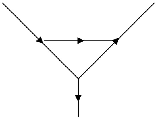
Figure 1.
The upper vertex of the diagram depicted in the right panel of Figure 2 but with arbitrary complex masses, , considered. The arrows indicate the flow of momenta.
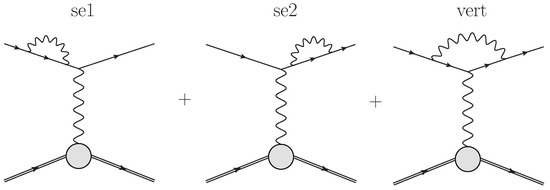
Figure 2.
Feynman diagrams describing the QED one-loop corrections at the lepton line in scattering. The arrows indicate the flow of momenta. This figure is from Ref. [32] and is used with the kind permission of The European Physical Journal A.
In this case, the vanishing cycles arise in any number of propagators from 2 to d. For definiteness, let us consider the propagators given by
The variety corresponding to this ideal is equivalent to the one generated by
or
where denotes the component of q that lies in the space spanned by , and is the component of q lying in a subspace orthogonal to the space spanned by .
If the Gram determinant of the system (33) is , this corresponds to a vanishing cycle at infinity (the stratum in the compactification of the q-space). We consider the case when . Then, is uniquely determined, and the equation for the singularity is the following:
where the determinant has a size of . We can now rewrite the integral in (30) as follows:
where
and is a smooth function equal to the product of the propagators, which are not part of the pinch (I is a set of propagators participating in the pinch). We then introduce the notation
where are the solutions of the following equation (the third one of the system (33)):
This is a point to which the vanishing cycle becomes contractible (the pinch point in our terminology). We also need to perform the following change in variables:
In all these variables, the integral in (35) transforms into
which can be reduced to
where is a regular function near the Landau variety . In (42), we have
with
Note that
where is the k-volume spanned by the vectors , and
One can also indicate that the first are coordinates on the space spanned by . The quantity vanishes identically on . In fact, it is proportional to the polynomial . At the end, we wish to emphasize that the integral in (42) has the following asymptotic expansion:
where is the volume dependent on dimensionality. is just the propagator evaluated at .
5.2. Propagator at Two Loops: General Case
Herein, we begin with the integral of the two-loop propagator, the diagram of which is shown in Figure 3:
We will focus on the vanishing cycle in
Here, the pinch point is
which is a solution of the system (49) for some scalar and where the singularity locus is at
The integral coefficient in the series expansion (explained in Theorem 3) is expressed as
and this integral coefficient is a function of masses and dimension only, with being one of the pinch points. In this case, the quadratic form and -term (see Theorem 3 again) are given by
where is the Landau polynomial [92], which is obtained by eliminating from the system (49):
where in Equations (54) and (55) are certain algebraic expressions deduced as a result of the above-mentioned elimination. The full expansion has the following form:
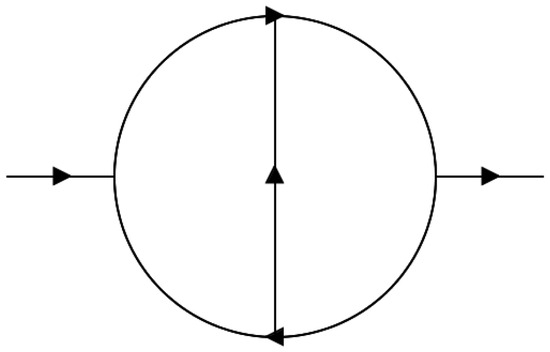
Figure 3.
A diagram describing the two-loop propagator but with arbitrary complex masses, , considered.
5.3. Vertex Diagram at Two Loops
5.3.1. General Case
Vertex diagrams at two loops, such as the example shown in Figure 4, have the following master integral form:
such that there are six given propagators in the integrand’s denominator:
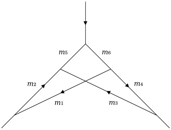
Figure 4.
The vertex diagram shown in Figure 5b but with arbitrary complex masses considered.
The case of QED-vertex two-loop diagrams, shown in Figure 5, corresponds to a particular choice of masses with . It matches up to a singular stratum in a diagram with generic masses, e.g, in the generalized diagram of Figure 4, there is a singularity at . In the corresponding QED diagram (Figure 5b in this case), we first restrict to the stratum and then perform analytic continuation.
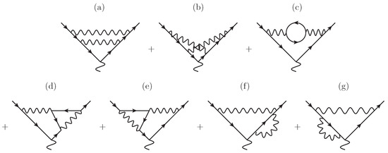
Figure 5.
Feynman diagrams describing QED two-loop corrections at the lepton line in scattering. The diagrams in the subfigures (a–g) constitute complete list of two-loop corrections to the QED vertex, and are important in the scattering theory because those constitute the sef of model independent corrections. We refer to Ref. [32] for more details. This figure is from Ref. [32] and is used with the kind permission of The European Physical Journal A.
Let us now concisely discuss the two-pinch singularity of the two-loop topology with the crossed vertex. We focus on the vanishing cycle by considering the two-pinch with the following propagators:
The pinch happens at
for which we make the change in variables of
Then, we have
or
which reduces to
where
that is, the corresponding Landau polynomial. The asymptotic solution corresponding to (64) is
which is similar to the formula (56).
5.3.2. Five-Pinch Point for Arbitrary Mass Vertex
In an asymptotic analysis of the arbitrary-mass two-loop ladder crossed vertex as shown in Figure 4, the geometry of the Landau varieties simplifies, such that it is possible to carry out the analysis of the five-pinch point explicitly. In this case, we consider the five-pinch point by the following propagators:
We have the pinch condition of
For example, (68) and the first two formulas of (67),
allow us to determine and . Analogously, (68) and the third and fourth formulas of (67),
allow to determine and .
The asymptotic analysis for the arbitrary mass vertex proceeds as follows. Near the pinch points and , we have the following integral:
which can be rewritten as
where and are -dependent residues. In general, the subscripts and in our formulas mean components of the orthogonal decomposition of the vector v with respect to the space spanned by , respectively.
In this expression, a determinant with vector entries has the following meaning. The vectors are essentially two-dimensional (due to Landau conditions, they are always a linear combination of ). Then, a column in which the combination of and occurs is meant to be split in two columns containing the coefficients in front of and , respectively. The general formula is in the Theorem 3.
For the leading order in the expansion parameter (the formula defining the Landau polynomial in (74)), Equation (72) reduces to
Note that in this case we have a determinantal formula for the Landau polynomial up to an overall factor A, which is a rational factor:
The Landau polynomial in (74) is considerably more complicated than that in the case of QED, derived in Section 5.3.4.
The determinant in the integral of (73) has the following explicit form:
where , are the elements of the last column, and the pinch points are given by
5.3.3. QED Case
We proceed by considering the above-mentioned QED two-loop crossed vertex diagram in Figure 5a as a specific example. This part of our analysis is a classical one, which may be compared to [93,94]. In this case, the integral of the vertex diagram is obtained from (67) by taking the limit , , .
Note that the mass limit is obtained by taking the limit on the integrand first. If we were to take the integral and then take the limit, we would observe a singularity in on an unphysical sheet.
We focus on the pinch point by the two fermion propagators and . Using the designation
the pinch occurs at
and at
The subtlety here is that the two pinch points in each of the variables coincide with each other, and there is an extra singularity coming from the photon propagator. We then use the following change in variables:
where lies in the subspace spanned by q. After this change in variables, we obtain
where one needs to compute the asymptotics at . The factor comes from evaluated at . The power counting gives for .
which eventually gives
with as a d-dependent factor.
5.3.4. Five-Pinch Point for QED Vertex
In an asymptotic analysis of the two-loop ladder contribution to the QED vertex with two massless lines as shown in Figure 5b, there is a direct analogy with what is already discussed in Section 5.3.2. In this case, the five-pinch point is given by the following propagators:
The pinch condition is given by the same formula (68):
Due to another condition of , one can write
where
where is the square root of the Gram matrix of (the signs ± could be chosen independently for ). We can also explicitly solve for as follows:
Then, the Landau polynomial for the five-pinch point is derived as follows:
in which there are polynomials for each choice of the signs of .
The asymptotic analysis for the QED vertex holds similarly to the analysis for the arbitrary mass vertex discussed in Section 5.3.2. We have the following integral near the pinch points and :
The evaluation of this determinant gives
where are the elements of the last column, and the pinch points are given by
Ultimately, we obtain up to a factor:
In (95), is proportional to the corresponding Landau polynomial :
where B is some algebraic function.
We should note that analogous expressions for the general mass case are more complicated and are much longer, which is the reason we do not write them after Equation (76) in Section 5.3.2.
6. Outlining the Method of Series for Performing Potentially New Types of Lepton–Proton Cross-Section Calculations in the Future
In this section, we concisely describe our vision for the use of the so-called -series method, how it ties in with the vanishing-cycle analysis discussed in Section 3 and Section 4, and how to employ it for future computations of the scattering amplitudes and cross-sections with lowest- and higher-order radiative corrections in scattering processes. Some diagrams presented in Section 5 are just examples of how we shall be treating them in our framework; nevertheless, for the cross-section calculations, much work still needs to be carried out. Here, we conjecture about such a possible future developments because neither this particular section nor the other parts of this paper address cross-sections or any other physical observables. Additionally, our current discussion is somewhat generic.
Notwithstanding that, at this point, one can outline some features in the -series method. This method is very well adapted to the calculation of hypergeometric (HG) Euler integrals with free polynomials in the integrand. In this case, it is possible to exhibit a basis of solutions of the corresponding holonomic system given by series via Ore–Sato coefficients [95]:
which is associated with a lattice, L. In our case, it is a lattice dual to the lattice generated by the Minkowski sum of Newton polytopes of the Feynman quadrics.
In fact, HG series have long been applied to Feynman integrals (see, e.g., [96,97]), and especially in recent years, this approach has been revived and systematically developed [11,13,14,56]. So, in Formula (97), is a lattice dual to L; the term is the Ore–Sato coefficients; v is the so-called initial monomials; is specific to an HG system and in physical applications is a function of the regulator; and runs over the lattice . The fact that such formulas unify many known expressions in particle physics can be indicated by the fact that the Ore–Sato coefficients, on one hand, provide the dimensional regularization of ultraviolet (UV) and infrared (IR) divergent integrals and, on the other hand, naturally include the -coefficients of functions on number fields in the context of HG motives [98].
In this paper, we focus on the asymptotic region near single Landau varieties or, stated in more technical terms, on the asymptotic analysis of the codimension 1 near Landau varieties. In this case, such an asymptotic aspect is rather simple: for regular a and b. Therefore, we do not really use any series, which is another factor to consider. At this point, the relationship of our vanishing cycle analysis to series is somewhat complicated because series construct the duality to an asymptotic analysis near intersections of several components of Landau hypersurfaces. We are going to elaborate on this in a future publication. In particular, for the case of one-loop functions, the correspondence between Landau varieties and series has been taken much further in [99]. In that case, the Landau varieties are strata of minuscule Grassmannians, and a one-loop function is obtained as a lift of a logarithmic bundle on the iterated covers that are branched with the degree 2 on the Landau varieties. Stated generally, the vanishing cycles correspond to the expansion of series near codimension-1 strata, while the series contain precise branching information near deeper strata.
The above considerations are valid only for the generic stratum, where the coefficients of the Feynman quadrics can be deformed away from the physical locus [61]. This locus, in turn, is a tiny subspace inside the universal deformation. Therefore, for achieving physical results, it is necessary to make use of the machinery of b-functions [100]. From a geometric point of view, we have to consider the restriction of the flat GZK bundle to a deep stratum. The most naive practical way to realize this is to start with the Gauss–Manin connection on the generic stratum and restrict it to the physical stratum. One complication is that the explicit form of this connection is not known, and a substantial development of the GZK formalism is needed for accomplishing it.
Furthermore, still from the geometric point of view, it is crucial to consider the uniformization of the singularity loci and the lift of the bundle to such uniformization. On general grounds, one can expect that such uniformization is achieved by -functions [101]. This is well known for single-variate polynomials [101,102,103]. However, we need to have its multivariate analogy at our disposal, which requires significant reformulation of the formalism. Note that the series constructed in the latter-cited papers are particular cases of series.
When applied to concrete-amplitude and cross-section calculations with lowest- and higher-order radiative corrections, e.g., in scattering, then along with carrying out the above analysis, we will also require an intimate study of the geometry of Landau polynomials, such as those shown in Formulas (55), (65), (74), and (90).
7. Discussion
In this paper, we used the Mayer–Vietoris spectral sequence for analyzing the vanishing cycles of Feynman integrals in Section 3 and Section 4, where we also gave a complete classification of the singularity development mechanisms. In Section 4.1, we obtained a general theorem of the localization of vanishing cycles in the integrals of polynomials. In Section 4.2, we obtained an integral representation for the coefficients of such an asymptotic expansion, as well as an asymptotic expression for integrals with generic polynomials (a result that seems to be new in the mathematical literature). In the whole of Section 5, we presented computations of some example diagrams in the case of arbitrary complex masses and QED, based on our findings in the previous sections. The novelty of this paper could be considered the approach used to carry out an asymptotic analysis that employs the momentum representation, where the Feynman parameter representation is usually employed.
As it is mentioned in Section 6, along with a future development of the entire ansatz, one of our future tasks shall be practical computations of one- and two-loop Feynman diagrams, as well as other next-to-leading and higher-order diagrams, for studies of radiative corrections in lepton–hadron scattering processes. We hope that such a new method, along with the theoretical ones existing in the literature [29,30,31,32,33,34,35,36], will be useful for any upcoming scattering experiments, such as PRad-II, Compass++/AMBER, PRES, MAGIX, and ULQ2, that will be devoted to measurements of the root-mean-square charge radius of the proton [104].
Author Contributions
Conceptualization, S.S. and V.K.; methodology, S.S.; validation, S.S. and V.K.; formal analysis, S.S.; investigation, S.S. and V.K.; resources, S.S.; writing—original draft preparation, S.S. and V.K.; writing—review and editing, S.S. and V.K.; visualization, S.S. and V.K.; supervision, S.S. and V.K.; funding acquisition, S.S. All authors have read and agreed to the published version of the manuscript.
Funding
This research received no external funding.
Data Availability Statement
This paper has no associated data, neither used in any form nor produced in the results.
Conflicts of Interest
The authors declare no conflicts of interest.
References
- Fotiadi, D.; Froissart, M.; Lascoux, J.; Pham, F. Applications of an isotopy theorem. Topology 1965, 4, 159–191. [Google Scholar] [CrossRef]
- Pham, F. Singularities of Integrals: Homology, Hyperfunctions and Microlocal Analysis; Springer Science & Business Media: Berlin/Heidelberg, Germany, 2011. [Google Scholar]
- Leray, J. Le calcul différentiel et intégral sur une variété analytique complexe.(Problème de Cauchy. III.). Bull. Soc. Math. Fr. 1959, 87, 81–180. [Google Scholar] [CrossRef]
- Kashiwara, M. B-functions and holonomic systems. Invent. Math. 1976, 38, 33–53. [Google Scholar] [CrossRef]
- Hwa, R.C.; Teplitz, V.L. Homology and Feynman integrals. Nucl. Phys. A 1967, 98, 627. [Google Scholar]
- Kontsevich, M. Intersection theory on the moduli space of curves and the matrix Airy function. Commun. Math. Phys. 1992, 147, 1–23. [Google Scholar] [CrossRef]
- Eden, R.J.; Landshoff, P.V.; Olive, D.I.; Polkinghorne, J.C. The Analytic S-Matrix; Cambridge University Press: Cambridge, UK, 2002. [Google Scholar]
- Griffiths, P.A. Periods of integrals on algebraic manifolds, I. (construction and properties of the modular varieties). Am. J. Math. 1968, 90, 568–626. [Google Scholar] [CrossRef]
- Manin, Y.I. Algebraic curves over fields with differentiation. Izv. Ross. Akad. Nauk. Seriya Mat. 1958, 22, 737–756. [Google Scholar]
- Gelfand, I.; Kapranov, M.; Zelevinskii, A. Discriminants, Resultants, and Multidimensional Determinants; Springer: Berlin/Heidelberg, Germany, 1994. [Google Scholar]
- Ananthanarayan, B.; Banik, S.; Bera, S.; Datta, S. FeynGKZ: A Mathematica package for solving Feynman integrals using GKZ hypergeometric systems. Comput. Phys. Commun. 2023, 287, 108699. [Google Scholar] [CrossRef]
- Fevola, C.; Mizera, S.; Telen, S. Principal Landau determinants. Comput. Phys. Commun. 2024, 303, 109278. [Google Scholar] [CrossRef]
- de la Cruz, L. Feynman integrals as A-hypergeometric functions. J. High Energy Phys. 2019, 2019, 123. [Google Scholar] [CrossRef]
- Feng, T.F.; Chang, C.H.; Chen, J.B.; Zhang, H.B. GKZ-hypergeometric systems for Feynman integrals. Nucl. Phys. B 2020, 953, 114952. [Google Scholar] [CrossRef]
- Mühlbauer, M. Cutkosky’s theorem for massive one-loop Feynman integrals: Part 1. Lett. Math. Phys. 2022, 112, 118. [Google Scholar] [CrossRef]
- Pathak, T.; Sreekantan, R. Singularities of Feynman Integrals. Eur. Phys. J. Spec. Top. 2024, 233, 2037–2055. [Google Scholar] [CrossRef]
- Yelleshpur Srikant, A. Spherical Contours, IR Divergences and the geometry of Feynman parameter integrands at one loop. J. High Energy Phys. 2020, 2020, 236. [Google Scholar] [CrossRef]
- Dlapa, C.; Henn, J.; Yan, K. Deriving canonical differential equations for Feynman integrals from a single uniform weight integral. J. High Energy Phys. 2020, 2020, 25. [Google Scholar] [CrossRef]
- Smirnov, A.; Smirnov, V. How to choose master integrals. Nucl. Phys. B 2020, 960, 115213. [Google Scholar] [CrossRef]
- Hannesdottir, H.S.; McLeod, A.J.; Schwartz, M.D.; Vergu, C. Implications of the Landau equations for iterated integrals. Phys. Rev. D 2022, 105, L061701. [Google Scholar] [CrossRef]
- Bourjaily, J.L.; Hannesdottir, H.; McLeod, A.J.; Schwartz, M.D.; Vergu, C. Sequential Discontinuities of Feynman Integrals and the Monodromy Group. J. High Energy Phys. 2021, 2021, 205. [Google Scholar] [CrossRef]
- Aoyama, T.; Hayakawa, M.; Kinoshita, T.; Nio, M. Tenth-order QED contribution to the electron g-2 and an improved value of the fine structure constant. Phys. Rev. Lett. 2012, 109, 111807. [Google Scholar] [CrossRef]
- Aoyama, T.; Asmussen, N.; Benayoun, M.; Bijnens, J.; Blum, T.; Bruno, M.; Caprini, I.; Calame, C.C.; Cè, M.; Colangelo, G.; et al. The anomalous magnetic moment of the muon in the Standard Model. Phys. Rep. 2020, 887, 1–166. [Google Scholar] [CrossRef]
- Jegerlehner, F. The Anomalous Magnetic Moment of the Muon; Springer: Berlin/Heidelberg, Germany, 2008. [Google Scholar]
- Keshavarzi, A.; Nomura, D.; Teubner, T. Muon g- 2 and α (M Z 2): A new data-based analysis. Phys. Rev. D 2018, 97, 114025. [Google Scholar] [CrossRef]
- Campbell, M.J.; Ellis, R.K.; Williams, C. Associated production of a Higgs boson at NNLO. J. High Energy Phys. 2016, 2016, 179. [Google Scholar] [CrossRef]
- Hessenberger, S.; Hollik, W. Two-loop improved predictions for MW and sin2 θeff in Two-Higgs-Doublet models. Eur. Phys. J. C 2022, 82, 970. [Google Scholar] [CrossRef]
- Ahmed, T.; Ravindran, V.; Sankar, A.; Tiwari, S. Two-loop amplitudes for di-Higgs and di-pseudo-Higgs productions through quark annihilation in QCD. J. High Energy Phys. 2022, 2022, 189. [Google Scholar] [CrossRef]
- Maximon, L.C.; Tjon, J.A. Radiative corrections to electron proton scattering. Phys. Rev. C 2000, 62, 054320. [Google Scholar] [CrossRef]
- Gramolin, A.V.; Fadin, V.S.; Feldman, A.L.; Gerasimov, R.E.; Nikolenko, D.M.; Rachek, I.A.; Toporkov, D.K. A new event generator for the elastic scattering of charged leptons on protons. J. Phys. G 2014, 41, 115001. [Google Scholar] [CrossRef]
- Akushevich, I.; Gao, H.; Ilyichev, A.; Meziane, M. Radiative corrections beyond the ultra relativistic limit in unpolarized ep elastic and Møller scatterings for the PRad Experiment at Jefferson Laboratory. Eur. Phys. J. A 2015, 51, 1. [Google Scholar] [CrossRef]
- Bucoveanu, R.D.; Spiesberger, H. Second-Order Leptonic Radiative Corrections for Lepton-Proton Scattering. Eur. Phys. J. A 2019, 55, 57. [Google Scholar] [CrossRef]
- Fadin, V.S.; Gerasimov, R.E. On the cancellation of radiative corrections to the cross section of electron-proton scattering. Phys. Lett. B 2019, 795, 172–176. [Google Scholar] [CrossRef]
- Banerjee, P.; Engel, T.; Signer, A.; Ulrich, Y. QED at NNLO with McMule. SciPost Phys. 2020, 9, 027. [Google Scholar] [CrossRef]
- Afanasev, A.; Ilyichev, A. Radiative corrections to the lepton current in unpolarized elastic lp-interaction for fixed Q2 and scattering angle. Eur. Phys. J. A 2021, 57, 280. [Google Scholar] [CrossRef]
- Kaiser, N.; Lin, Y.H.; Meißner, U.G. Radiative corrections to elastic muon-proton scattering at low momentum transfers. Phys. Rev. D 2022, 105, 076006. [Google Scholar] [CrossRef]
- Shumeiko, N.M.; Suarez, J.G. The QED lowest order radiative corrections to the two polarized identical fermion scattering. J. Phys. G 2000, 26, 113–127. [Google Scholar] [CrossRef]
- Kaiser, N. Radiative corrections to lepton-lepton scattering revisited. J. Phys. G 2010, 37, 115005. [Google Scholar] [CrossRef]
- Aleksejevs, A.G.; Barkanova, S.G.; Zykunov, V.A.; Kuraev, E.A. Estimating two-loop radiative effects in the MOLLER experiment. Phys. Atom. Nucl. 2013, 76, 888–900. [Google Scholar] [CrossRef]
- Aleksejevs, A.G.; Barkanova, S.G.; Bystritskiy, Y.M.; Zykunov, V.A. One-Loop Electroweak Radiative Corrections to Bhabha Scattering in the Belle II Experiment. Phys. Part. Nucl. 2020, 51, 645–650. [Google Scholar] [CrossRef]
- Zykunov, V.A. Radiative Corrections in Møller Scattering for PRad Experiment at Thomas Jefferson National Accelerator Facility (TJNAF). Phys. At. Nucl. 2021, 84, 739–749. [Google Scholar] [CrossRef]
- Banerjee, P.; Engel, T.; Schalch, N.; Signer, A.; Ulrich, Y. Møller scattering at NNLO. Phys. Rev. D 2022, 105, L031904. [Google Scholar] [CrossRef]
- Bondarenko, S.G.; Kalinovskaya, L.V.; Rumyantsev, L.A.; Yermolchyk, V.L. One-loop electroweak radiative corrections to polarized Møller scattering. arXiv 2022, arXiv:2203.10538. [Google Scholar] [CrossRef]
- Frellesvig, H.; Gasparotto, F.; Laporta, S.; Mandal, M.K.; Mastrolia, P.; Mattiazzi, L.; Mizera, S. Decomposition of Feynman Integrals by Multivariate Intersection Numbers. J. High Energy Phys. 2021, 2021, 27. [Google Scholar] [CrossRef]
- Frellesvig, H.; Gasparotto, F.; Mandal, K.M.; Mastrolia, P.; Mattiazzi, L.; Mizera, S. Vector Space of Feynman Integrals and Multivariate Intersection Numbers. Phys. Rev. Lett. 2019, 123, 201602. [Google Scholar] [CrossRef] [PubMed]
- Di Vita, S.; Laporta, S.; Mastrolia, P.; Primo, A.; Schubert, U. Master integrals for the NNLO virtual corrections to μe scattering in QED: The non-planar graphs. J. High Energy Phys. 2018, 2018, 16. [Google Scholar] [CrossRef]
- Bonisch, K.; Fischbach, F.; Klemm, A.; Nega, C.; Safari, R. Analytic structure of all loop banana integrals. J. High Energy Phys. 2021, 2021, 66. [Google Scholar] [CrossRef]
- Remiddi, E.; Tancredi, L. Schouten identities for Feynman graph amplitudes; The Master Integrals for the two-loop massive sunrise graph. Nucl. Phys. B 2014, 880, 343–377. [Google Scholar] [CrossRef]
- Chaubey, E.; Weinzierl, S. Two-loop master integrals for the mixed QCD-electroweak corrections for through a -coupling. J. High Energy Phys. 2019, 2019, 185. [Google Scholar] [CrossRef]
- Pogel, S.; Wang, X.; Weinzierl, S. The three-loop equal-mass banana integral in ε-factorised form with meromorphic modular forms. J. High Energy Phys. 2022, 2022, 62. [Google Scholar] [CrossRef]
- Weinzierl, S. Modular transformations of elliptic Feynman integrals. Nucl. Phys. B 2021, 964, 115309. [Google Scholar] [CrossRef]
- Bloch, S.; Kerr, M.; Vanhove, P. A Feynman integral via higher normal functions. Compos. Math. 2015, 151, 2329–2375. [Google Scholar] [CrossRef]
- Bloch, S.; Kerr, M.; Vanhove, P. Local mirror symmetry and the sunset Feynman integral. Adv. Theor. Math. Phys. 2017, 21, 1373–1453. [Google Scholar] [CrossRef]
- de la Cruz, L.; Vanhove, P. Algorithm for differential equations for Feynman integrals in general dimensions. Lett. Math. Phys. 2024, 114, 89. [Google Scholar] [CrossRef]
- Pögel, S.; Wang, X.; Weinzierl, S. Bananas of equal mass: Any loop, any order in the dimensional regularisation parameter. J. High Energy Phys. 2023, 2023, 117. [Google Scholar] [CrossRef]
- Klausen, R.P. Hypergeometric Series Representations of Feynman Integrals by GKZ Hypergeometric Systems. J. High Energy Phys. 2020, 2020, 121. [Google Scholar] [CrossRef]
- Pögel, S.; Wang, X.; Weinzierl, S. Taming Calabi-Yau Feynman Integrals: The Four-Loop Equal-Mass Banana Integral. Phys. Rev. Lett. 2023, 130, 101601. [Google Scholar] [CrossRef] [PubMed]
- Gelfand, I.; Zelevinskii, A.; Kapranov, M. Hypergeometric functions and toral manifolds. Funct. Anal. Its Appl. 1989, 23, 94–106. [Google Scholar] [CrossRef]
- Saito, M.; Sturmfels, B.; Takayama, N. Grobner Deformations of Hypergeometric Differential Equations; Springer Science & Business Media: Berlin/Heidelberg, Germany, 2013; Volume 6. [Google Scholar]
- Hibi, T.; Nishiyama, K.; Takayama, N. Pfaffian systems of A-hypergeometric equations I: Bases of twisted cohomology groups. Adv. Math. 2017, 306, 303–327. [Google Scholar] [CrossRef]
- Srednyak, S. Universal deformation of particle momenta space in perturbation theory. arXiv 2018, arXiv:1805.00433. [Google Scholar]
- Kashiwara, M. D-Modules and Microlocal Calculus; American Mathematical Soc.: Providence, RI, USA, 2003; Volume 217. [Google Scholar]
- Hotta, R.; Tanisaki, T. D-Modules, Perverse Sheaves, and Representation Theory; Springer Science & Business Media: Berlin/Heidelberg, Germany, 2007; Volume 236. [Google Scholar]
- Gelfand, I.M.; Kapranov, M.M.; Zelevinsky, A.V.; Gelfand, I.M.; Kapranov, M.M.; Zelevinsky, A.V. A-Discriminants; Springer: Berlin/Heidelberg, Germany, 1994. [Google Scholar]
- Arnold, V.; Gusein-Zade, S.; Varchenko, A. Singularities of Differentiable Maps: Volume II Monodromy and Asymptotic Integrals; Springer Science & Business Media: Berlin/Heidelberg, Germany, 2012; Volume 83. [Google Scholar]
- Kashiwara, M.; Schapira, P. Regular and Irregular Holonomic D-Modules; Cambridge University Press: Cambridge, UK, 2016; Volume 433. [Google Scholar]
- Deligne, P. Équations Différentielles à Points Singuliers Réguliers; Springer: Berlin/Heidelberg, Germany, 2006; Volume 163. [Google Scholar]
- Adams, L.; Bogner, C.; Weinzierl, S. The two-loop sunrise graph in two space-time dimensions with arbitrary masses in terms of elliptic dilogarithms. J. Math. Phys. 2014, 55, 102301. [Google Scholar] [CrossRef]
- Dimca, A. Singularities and Topology of Hypersurfaces; Springer Science & Business Media: Berlin/Heidelberg, Germany, 1992. [Google Scholar]
- Spanier, E.H. Algebraic Topology; Springer Science & Business Media: Berlin/Heidelberg, Germany, 1989. [Google Scholar]
- Bogner, C.; Weinzierl, S. Feynman graph polynomials. Int. J. Mod. Phys. A 2010, 25, 2585–2618. [Google Scholar] [CrossRef]
- Bott, R.; Tu, L.W. Differential Forms in Algebraic Topology; Springer: Berlin/Heidelberg, Germany, 1982; Volume 82. [Google Scholar]
- Libgober, A. Homotopy groups of the complements to singular hypersurfaces, II. Ann. Math. 1994, 139, 117–144. [Google Scholar] [CrossRef]
- Dimca, A.; Papadima, Ş.; Suciu, A.I. Topology and geometry of cohomology jump loci. Duke Math. J. 2009, 148, 405–457. [Google Scholar] [CrossRef]
- Brown, F. Mixed Tate motives over Z. Ann. Math. 2012, 175, 949–976. [Google Scholar] [CrossRef]
- Beem, C.; Ben-Zvi, D.; Bullimore, M.; Dimofte, T.; Neitzke, A. Secondary products in supersymmetric field theory. In Annales Henri Poincaré; Springer: Berlin/Heidelberg, Germany, 2020; pp. 1235–1310. [Google Scholar]
- Peters, C.A.; Steenbrink, J.H. Mixed Hodge Structures; Springer Science & Business Media: Berlin/Heidelberg, Germany, 2008; Volume 52. [Google Scholar]
- Deligne, P.; Griffiths, P.; Morgan, J.; Sullivan, D. Real homotopy theory of Kähler manifolds. Invent. Math. 1975, 29, 245–274. [Google Scholar] [CrossRef]
- Schmid, W. Variation of Hodge structure: The singularities of the period mapping. Invent. Math. 1973, 22, 211–319. [Google Scholar] [CrossRef]
- Massey, D.B. Non-isolated hypersurface singularities and Lê cycles. Real Complex Singul. 2016, 675, 197–227. [Google Scholar]
- Bourjaily, J.L.; Vergu, C.; Von Hippel, M. Landau singularities and higher-order polynomial roots. Phys. Rev. D 2023, 108, 085021. [Google Scholar] [CrossRef]
- Seidel, P. Lagrangian homology spheres in (Am) Milnor fibres via C*–equivariant A_–modules. Geom. Topol. 2013, 16, 2343–2389. [Google Scholar] [CrossRef]
- Lê, D.; Perron, B. Sur la fibre de Milnor d’une singularité isolée en dimension complexe trois. CR Acad. Sci. Pairs Sér. A 1979, 289, 115–118. [Google Scholar]
- Mumford, D.; Fogarty, J.; Kirwan, F. Geometric Invariant Theory; Springer Science & Business Media: Berlin/Heidelberg, Germany, 1994; Volume 34. [Google Scholar]
- Milnor, J. Singular Points of Complex Hypersurfaces, (AM-61); Princeton University Press: Princeton, NJ, USA, 2016; Volume 61. [Google Scholar]
- Varchenko, A. On the local residue and the intersection form on the vanishing cohomology. Math. USSR-Izv. 1986, 26, 31. [Google Scholar] [CrossRef]
- Cattani, E.; Cueto, M.A.; Dickenstein, A.; Di Rocco, S.; Sturmfels, B. Mixed discriminants. Math. Z. 2013, 274, 761–778. [Google Scholar] [CrossRef]
- Dolotin, V.; Morozov, A. Introduction to non-linear algebra. arXiv 2006, arXiv:hep-th/0609022. [Google Scholar]
- Milnor, J. Whitehead torsion. Bull. Am. Math. Soc. 1966, 72, 358–426. [Google Scholar] [CrossRef]
- Anokhina, A.S.; Morozov, A.Y.; Shakirov, S.R. Resultant as the determinant of a Koszul complex. Theor. Math. Phys. 2009, 160, 1203–1228. [Google Scholar] [CrossRef]
- Srednyak, S. Feynman integrals as flat bundles over the complement of Landau varieties. arXiv 2017, arXiv:1710.09883. [Google Scholar] [CrossRef]
- Landau, L. On analytic properties of vertex parts in quantum field theory. Nucl. Phys 1960, 13, 181–192. [Google Scholar] [CrossRef]
- Sudakov, V.V. Vertex parts at very high energies in quantum electrodynamics. Zh. Eksp. Teor. Fiz. 1956, 3, 65–71. [Google Scholar]
- Gribov, V.N.; Lipatov, L.N. Deep Inelastic ep-Scattering in a Perturbation Theory; Technical Report; Inst. of Nuclear Physics: Leningrad, Russia, 1972. [Google Scholar]
- Gel’fand, I.M.; Graev, M.I.; Retakh, V.S. General hypergeometric systems of equations and series of hypergeometric type. Russ. Math. Surv. 1992, 47, 1. [Google Scholar] [CrossRef]
- Fleischer, J.; Jegerlehner, F.; Tarasov, O.V. A New hypergeometric representation of one loop scalar integrals in d dimensions. Nucl. Phys. B 2003, 672, 303–328. [Google Scholar] [CrossRef]
- Yost, S.A.; Bytev, V.V.; Kalmykov, M.Y.; Kniehl, B.A.; Ward, B.F.L. The Epsilon Expansion of Feynman Diagrams via Hypergeometric Functions and Differential Reduction. arXiv 2011, arXiv:1110.0210. [Google Scholar] [CrossRef]
- Beilinson, A.; Bloch, S.; Esnault, H. ϵ-factors for Gauss-Manin determinants. arXiv 2001, arXiv:math/0111277. [Google Scholar]
- Aomoto, K. Analytic structure of Schläfli function. Nagoya Math. J. 1977, 68, 1–16. [Google Scholar] [CrossRef]
- Saito, M. On microlocal b-function. Bull. Soc. Math. Fr. 1994, 122, 163–184. [Google Scholar] [CrossRef]
- Mumford, D.; Nori, M.; Norman, P. Tata Lectures on Theta III; Springer: Berlin/Heidelberg, Germany, 2007; Volume 43. [Google Scholar]
- Sturmfels, B. Solving algebraic equations in terms of A-hypergeometric series. Discret. Math. 2000, 210, 171–181. [Google Scholar] [CrossRef]
- Passare, M.; Sadykov, T.; Tsikh, A. Singularities of hypergeometric functions in several variables. Compos. Math. 2005, 141, 787–810. [Google Scholar] [CrossRef]
- Xiong, W.; Peng, C. Proton Electric Charge Radius from Lepton Scattering. Universe 2023, 9, 182. [Google Scholar] [CrossRef]
Disclaimer/Publisher’s Note: The statements, opinions and data contained in all publications are solely those of the individual author(s) and contributor(s) and not of MDPI and/or the editor(s). MDPI and/or the editor(s) disclaim responsibility for any injury to people or property resulting from any ideas, methods, instructions or products referred to in the content. |
© 2025 by the authors. Licensee MDPI, Basel, Switzerland. This article is an open access article distributed under the terms and conditions of the Creative Commons Attribution (CC BY) license (https://creativecommons.org/licenses/by/4.0/).