Abstract
The goal of this article is to reduce the vibration of a hybrid oscillator with a cubic–quintic nonlinear term under internal and external forces in the worst resonance case. To eliminate the harmful vibration in the system, the following strategies are suggested: nonlinear derivative feedback control (NDF), linear negative velocity feedback control (LNVC), nonlinear integral positive position feedback (NIPPF), integral resonant control (IRC), negative velocity with time delay (TD), and positive position feedback (PPF). It is discovered that the PPF control suppresses vibration more effectively than typical controllers, which reduces the vibration to 0.0001 with an effectiveness of 99.92%. Moreover, the main advantages of the PPF controller are its low cost and the fast response. The multiple time scale perturbation technique (MSPT) is used to apply the theoretical methodology and obtain a perturbed response. In order to close the concurrent primary and internal resonance case, frequency response (FR) equations are also used to study and analyze the system’s stability. The MATLAB software is used to complete and clarify all numerical topics. The FR curves are examined to determine the amplitude’s subsequent impact from variations in the parameters’ values. Lastly, a comparison of the numerical and analytical solutions is performed utilizing time history. Along with comparing the impact of our PPF damper on the hybrid oscillator, earlier research is also provided.
Keywords:
multiple scale perturbation technique (MSPT); linear negative velocity feedback (LNVC); positive position feedback (PPF); negative derivative feedback (NDF); resonance case; stability MSC:
65P40; 70K20; 74H10; 74H45
1. Introduction
One intriguing example that demonstrates the mathematical description of nonlinear phenomena present in a variety of scientific, physical, and engineering contexts is nonlinear vibration. Most machines, cars, buildings, structures, and dynamic systems vibrate, which is undesirable not only because of the unsightly motions that result but also because of the dynamic stresses that can cause fatigue and machine or structure failure, the energy losses and performance reduction that come with vibrations, and the noise that is produced, so we must eliminate or reduce these vibrations.
Nonlinear vibrations are present in both our daily lives and the devices we use for work. Because of their significance in examining various nonlinear sciences, electrical factory production, and manufacture, nonlinear oscillators are among the most significant and commonly use functioning prototypes in complex structures. The differential equation is one of the most famous and important equations, and its solution has been extremely important in the field of physics, engineering, and environment in recent years; many scholars have worked hard to develop a computational analytical, or semi-analytical, solution for this set of problems, in line with the differential equation type.
For instance, the N/MIEMS system exhibits nonlinear vibrations [1,2,3,4,5]. It is now possible to transform the Kundu–Mukherjee–Naskar equation’s nonlinear wave equation into a Duffing-like equation and the nonlinear vibration system in a porous media into a fractal modification [6,7,8]. The Duffing equation is used in a variety of circumstances, including electrical circuits, optical stability, buckling beams, and plasma oscillation [9]. For many years, applied mathematics, physics, practical engineering, and several real-world applications have relied heavily on nonlinear oscillations.
Nayfeh [10] and Mickens [11] achieved an approximation for nonlinear oscillators. An estimated bounded solution for parametric DEs was obtained by Motamid [12] by combining the Laplace transformation and homotopy perturbation method. The exact solution for the cubic DEs, which was obtained in this study, showed that the system is destabilized due to the damped variable and the cubic stiffness factor. In recent decades, the control of significantly forced systems has drawn a lot of attention from a range of real-world engineering fields. The primary organization of passive oscillation absorbers is associated with a physiological preparation, in contrast to automated frequency absorbers, which were replaced with a regulating structure made up of a sensor, actuators, and filters. The Van der Pol oscillator is a significant nonlinear oscillator that has received a lot of attention. The repercussions are still being dealt with today. The cubic–quintic Duffing–Van der Pol equation and two more periodic driving terms were investigated [13]. In order to improve the bandwidth position of a lightly damping resonant system, Russell et al. [14] implemented a modified IRC technique. Then, a technique that went against traditional IRC was developed to lower the controller’s order by a selective feed through selection. In order to provide the highest tracking bandwidth, controller parameters have subsequently been analytically determined.
Cveticanin et al. [15] looked at the periodic solution of a nonlinear oscillator that described the generalized Rayleigh equation. The vibration of the Van der Pol–Duffing–Rayleigh oscillator was controlled via two different time delays, one for position and one for velocity. A comparison of the numerous scales technique, harmonic balance, and the direct normal form technique was conducted by Hilla et al. [16]. Therefore, it has been determined that these approaches reflect sufficient accuracy for approaching backbone curves when the amplitude response is low, based on the investigation of unforced, undamped Duffing oscillators.
Huang et al. [17] employed delayed feedback to regulate the bifurcation of a fractional predator–prey system. Barron [18] examined the ring of connected Van der Pol oscillators’ dynamically stable and unstable behavior. He also mentioned mathematically that, if the stability requirements fail to be satisfied, the oscillator’s amplitude increases. The nonlinear dynamics of the “Hybrid Rayleigh–Van der Pol–Duffing oscillator” were studied by Miwadinou et al. [19]. They reported that there are nine resonance states in the system. They demonstrated that the resonance phenomena were robust in relation to the external force and nonlinear quadratic and cubic damping. Moreover, bifurcation was demonstrated using numerical simulations. A tuned dumber, also known as a passive control, was created to regulate the Van der Pol oscillator’s vibrations. PPF controllers with a time delay were used to reduce the vibrations of coupled Van der Pol oscillators. They demonstrated the effectiveness of PPF controllers with a time delay equal to 198.92 and 227.02 [20]. The performance of NDF and PPF controllers with a single-link flexible manipulator with a piezoelectric actuator is examined in [21]. NDF performs better than PPF, according to the study’s experimental comparison of their efficacity in terms of the settling time and vibration attenuation at different damping ratios. It was also the first to examine these controllers’ resilience to natural frequency vibrations in flexible manipulator systems. The NPA was used to drive an equivalent linear differential equation for structural analysis, showing high consistency with precise frequency results in numerical computations. Various control strategies were proposed, with NDF proving to be the most efficient for vibration reduction, by Moatimid et al. [22]. The PPF controller was employed by Jung et al. [23] to reduce the vibration of the strip. Conversely, EL-Ganaini et al. [24] studied a PPF controller with the goal of lowering the vibration amplitude of the nonlinear dynamical system when 1:1 IR and PR were present.
The NIPPF control, which combines the compensation of the PPF controller and IRC for nonlinear system control, has a significant impact since it lessens oscillation at the exact resonance frequency, as established by Omidi and Mahmoodi [25]. Regarding the Lyapunov approach, Kandil and El-Gohary [26] used proportional derivative control to examine the method’s delay time effect. The reduction in rotational beam oscillation at different speeds lessened this effect. The analytical solution was obtained by applying the multiple scales approach. To solve nonlinear differential equations and arrive at approximations, MSPT is employed. Among the most widely used perturbation techniques are multiple-scale approaches. These approaches generate both transient and steady-state solutions when used by [27], in comparison to certain alternative methods that solely offer the steady-state solution. Bauomy et al. [28] demonstrated that, in order to lessen the vibration response in a double Van der Pol oscillator that is excited by external stimuli, the integral resonant negative derivative feedback (IRNDF) controller can be additionally introduced. The IRNDF controller performs better than conventional controllers in reducing oscillations and amplitude values by combining integral resonant control with NDF. Strong agreement is shown via analytical and numerical investigation. Amer et al. [29] investigated how a piezoelectric device affected the two-DOF dynamical system’s planar motion. Under the influence of external forces and moments, this system consists of a nonlinear damping spring pendulum whose pivot point rotates counterclockwise at a constant angular velocity on a Lissajous curve. The MSPT is used to obtain the novel asymptotic solutions of the system up to the third approximation. The fourth-order Runge–Kutta method (RK-4) is used to drive the numerical solutions of the equations of motion. The FR curve showed several areas of stability and instability, demonstrating how different parameters affected the system’s dynamic behavior. Amer et al. [30] evolved a dynamical model using an MSPT of the shearer permanent magnetic tiny drive braking transmission. We looked into and figured out the multi-excitation force mechanism. The awful resonance incidences through the negative velocity feedback (NVF) and cubic velocity feedback (CVF) controllers were also covered. The relationship between the controller and the CVF controller becomes more apparent. They demonstrated that, when both external and parametric excitation forces are applied, the NVF controller works better for this system.
The study that was conducted by HS. Bauomy and A. EL-sayed [31] used NDF to reduce harmful vibrations. It looked at how to control and bifurcation-analyze a cart–pendulum system, which is a 2DOF model that is not fully actuated. In order to compare the analytical solutions for the nonlinear differential equations with numerical simultaneous using the Runge–Kutta method, the study used the averaging methodology, while stability and steady-state amplitude were evaluated both before and after control deployment.
In this study, a mathematical formulation for the system’s vibration with various controller types is presented. When compared to the uncontrolled situation, the PPF controller reduces the oscillator’s amplitude by 99.9%, making it the most effective of six controller choices. The flowchart structure of the system with three different controllers and a Poincaré system without and with a controller is presented. With the aid of an MSPT up to the first approximation, an approximate solution for the system coupled with the PPF controller is examined. Additionally, the equilibrium solution’s stability behavior under both primary and internal resonance conditions is examined. The impact of the chosen system parameters is demonstrated numerically in the study. The stability analyses of the ME are examined in accordance with the solutions in the steady-state scenario. Moreover, the stability of the nonlinear amplitudes within the modulation equations system and the attributes of nonlinear analysis are showcased through the utilization of complex transformations applied to the system’s amplitudes. Consequently, the resonance curves and the amplitude–frequency curves at various parameters are used to display the associated domains of stability and instability. The difference between the analytical and numerical solution is explained; in addition, it is shown how various factors affect the behavior of the system.
2. Mathematical Model and Controller Design
The equation of a hybrid Rayleigh–Van der Pol–Duffing oscillator that describes the physical model shown in [32] is given by the following:
where the displacement of the system is . The coefficient of nonlinear terms is and impure and pure quadratic damping coefficients, respectively; are impure and pure cubic damping coefficients. The excitation amplitude and frequency are .
2.1. Different Kinds of Control for the Equation of Motion
The modified equation of a hybrid oscillator system after adding different kind of controllers is as follows:
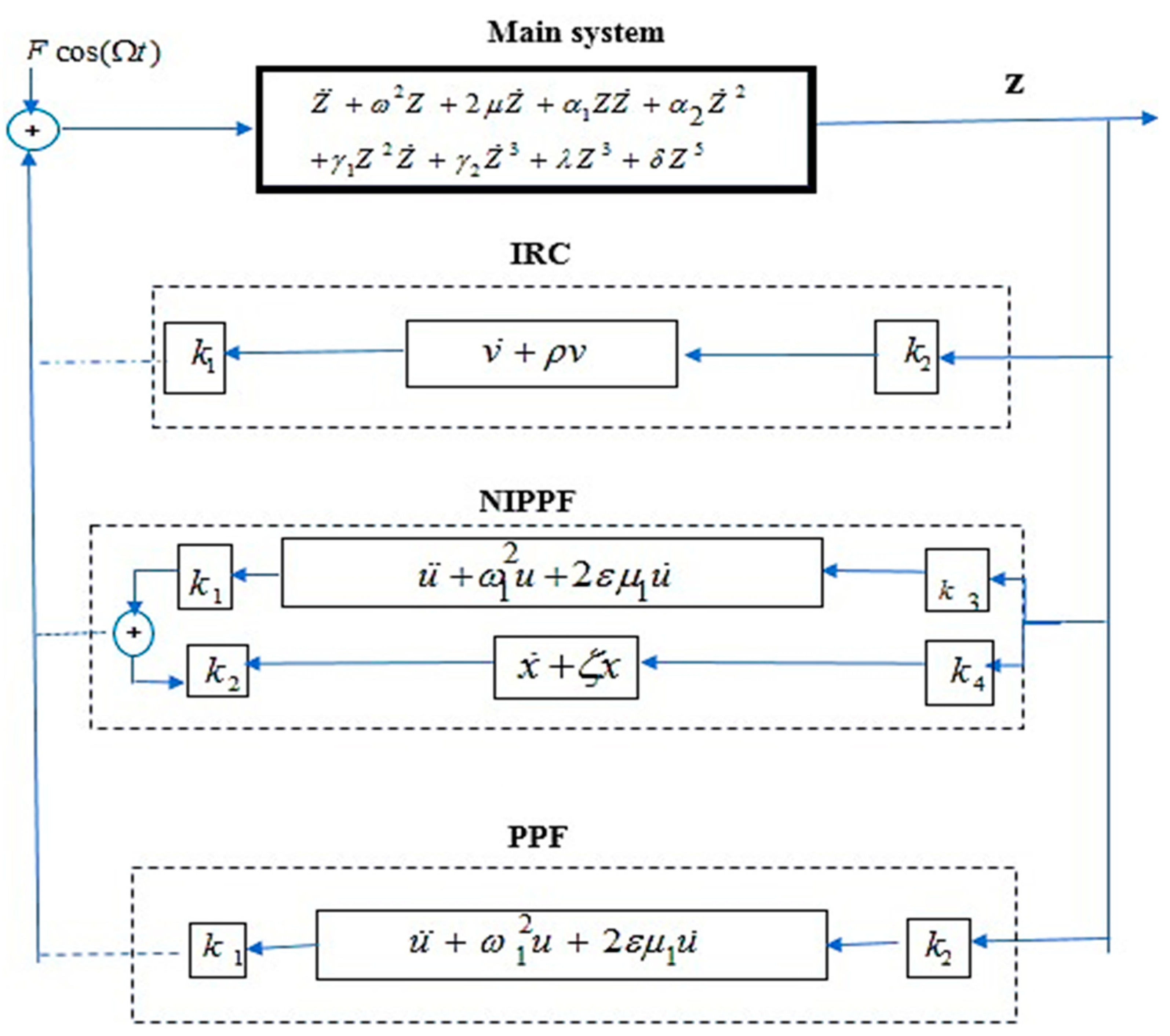
where is the control input, as shown in the flowchart in Figure 1, and it may represent the various kinds of control to reduce vibration as follows:
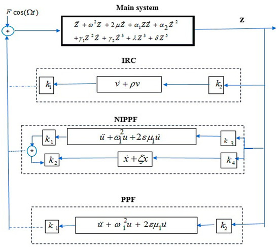
Figure 1.
Flowchart graph for the structure with three kinds of controllers.
- First kind: linear negative velocity feedback (LNVF),
- Second kind: integral resonant control (IRC),
- Third kind: negative velocity time delay (TD),
- Fourth kind: positive position feedback (PPF),
- Fifth kind: nonlinear integral positive position feedback (NIPPF),
- Sixth kind: negative derivative feedback (NDF),
2.2. Equation of Motion with Positive Position Feedback (PPF)
By conducting a numerical comparison adding different controller types into a hybrid oscillator system, shown in (Figure 27 and Table 1), we can conclude that PPF is the optimum control for this system under the specified parameter choice; hence, the equation of the motion becomes as follows:

Table 1.
Comparison between different types of controllers.
3. The Proposed Methodology for the Approximate Solution
In order to obtain an approximation solution for the nonlinear system that follows the PPF controller, which is the optimum controller compared to other types that are introduced in Equations (9) and (10), this part uses the MSPT [33]; the solutions and can be stated as illustrated below.
where is a perturbation parameter that is sufficiently important, and the derivatives, ; thus, the derivatives for the time equation will be realized as follows:
Equations (11)–(14) are substituted into Equations (9) and (10) so that the following applies:
Comparing the quantities of the equal power of
reveals
The following is obtained by resolving the homogeneous differential equations using Equations (17) and (18):
Inserting (21) and (22) into (19) and (20) results in the following:
After the secular terms are eliminated, the complex conjugate components are collected under the acronym CC, yielding the following forms:
From the first approximation, we infer the following reasoning:
- PR: .
- IR: .
- SR: .
We determine the solvability requirements of the system in the worst case and add the detuning parameters and to get the following:
Through the splitting of (25) and (26), the equation is separated into secular and tiny parts, including Equation (27). In order to determine the solvability conditions, the following steps are involved:
A and B are exchanged with the polar form as follows:
where the steady-state motion phases and amplitude are denoted as and , respectively. After combining Equations (30) and (31) into Equations (28) and (29), we can then equal the real and imaginary elements as follows:
where and . The preceding equation is displayed as follows:
When , in order to acquire the system’s steady-state solution using PPF controllers connected to the fixed point of (36)–(39), then the FR of the practical case () is as follows:
Squaring and adding together for (40)–(43) leads to the following:
Stability Criteria
To examine whether the non-linear solution of the derived fixed points is stable, let the following apply:
where and are solution of Equations (36)–(39), and the perturbations and are considered to be small compared to and . The following equations are obtained by substituting Equation (46) into (36)–(39), maintaining just the linear terms:
The following matrix form can be used to display Equations (47)–(50):
where (47)–(50) provides the Jacobian matrix coefficients for the system. The following eigenvalue equation can be expressed as follows:
Hence, (52) can be rewritten as follows:
where is defined in Appendix A. The periodic solution is stable if the real part of the eigenvalue is negative, as determined via the “Routh-Hurwitz” criterion; if not, it is unstable.
4. Results and Discussion
This section is devoted to examining the numerical solutions of the aforementioned system, (36)–(39), using the Runge–Kutta method from the fourth order with the help of the MATLAB R2023b software. It must be mentioned that these equations cannot be solved analytically to obtain the amplitudes and the modified phases and .
4.1. System Performance Both Without and with Control
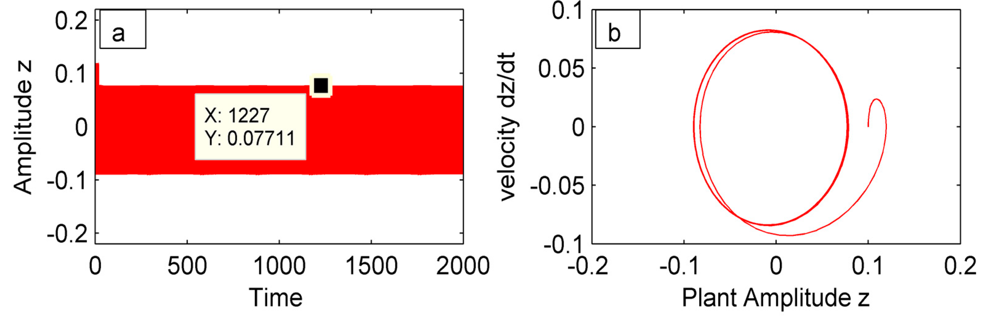
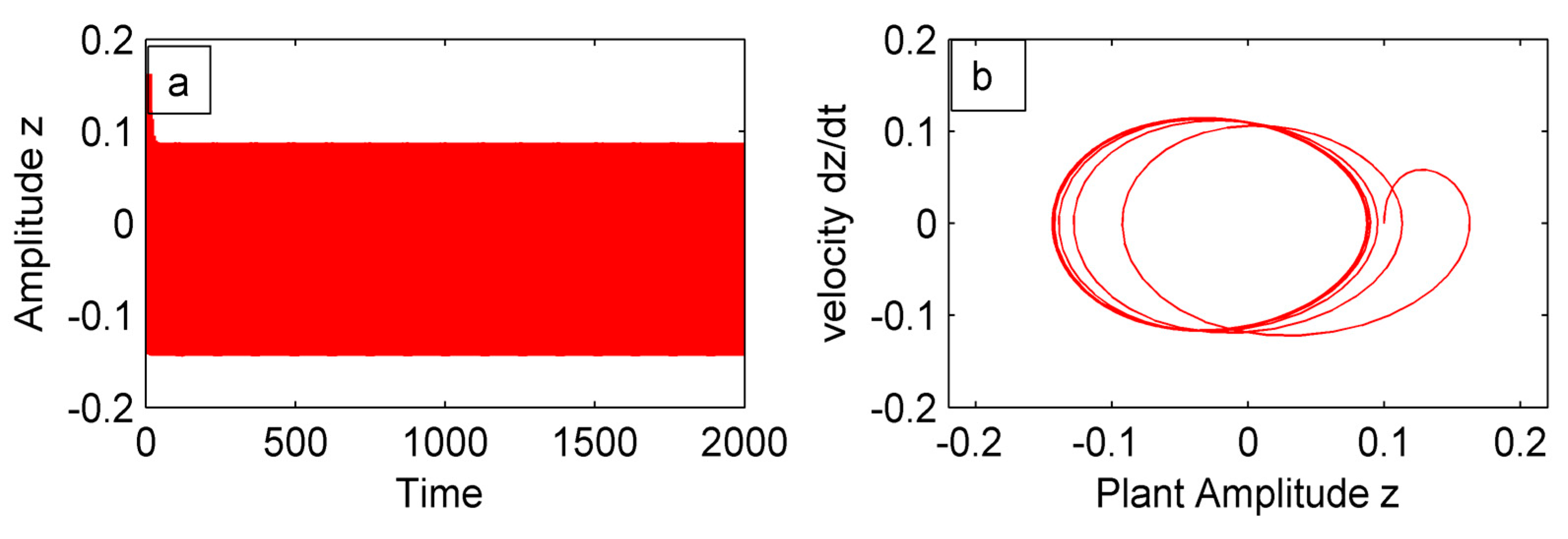
Studying the behavior of the system at the worst resonance cases, and , which are the combination of IR and PR cases, revealed that the absorber and system oscillations have many limit cycles and growing dynamic chaos. In order to reduce the vibration, these are the circumstances that need to be managed. By analyzing the amplitude of the PR system and selecting the worst case without an absorber, this was illustrated. This led to a comparison of the effectiveness of multiple controllers, and the best one was chosen in the case with the equation of motion, as illustrated in the adjacent figures. Figure 2 illustrates the amplitude of the main system without any resonance case and without control . The amplitude of the uncontrolled system is shown in Figure 3 before any type of controller is used at the primary resonance , which is the worst possible resonance case, and the range of amplitude is 0.1235. In Figure 4, after adding LNVF at the primary resonance case , we find that the amplitude decreases until it reaches 0.0771 and the effectiveness of controller .

Figure 2.
(a) Time history and (b) phase plane of the system without any resonance case and any control at ().

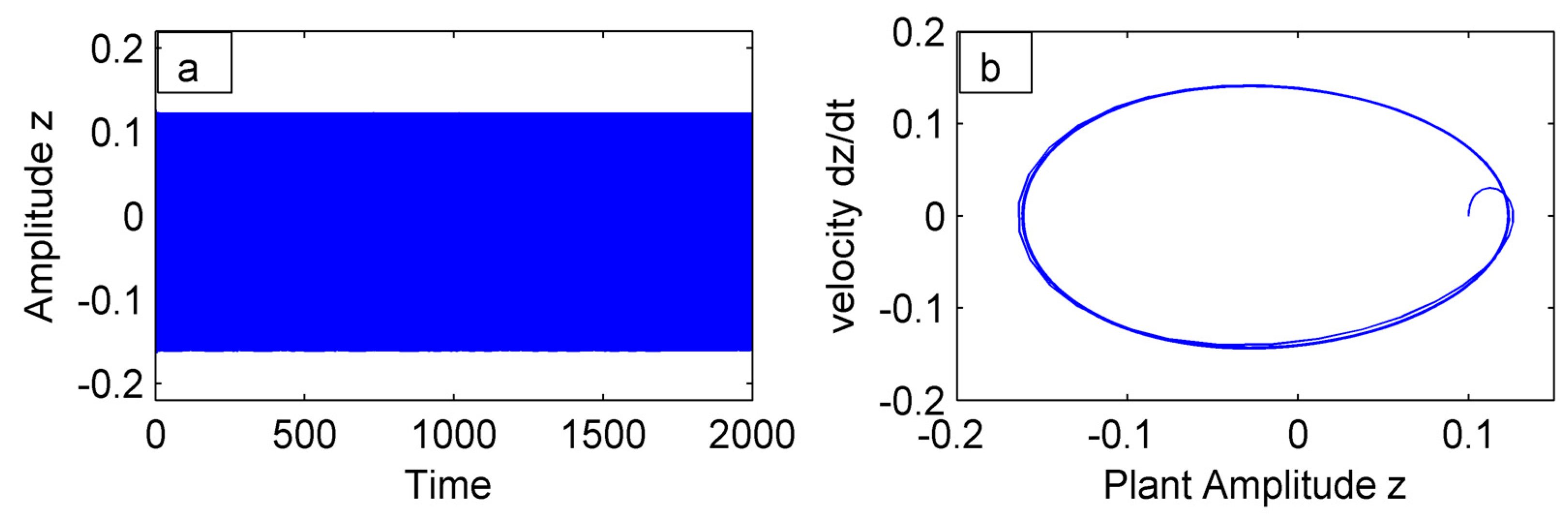
Figure 3.
(a) Time history and (b) phase plane of the system at primary resonance without control .

Figure 4.
(a) Time history and (b) phase plane of the system with LNVF at primary resonance .
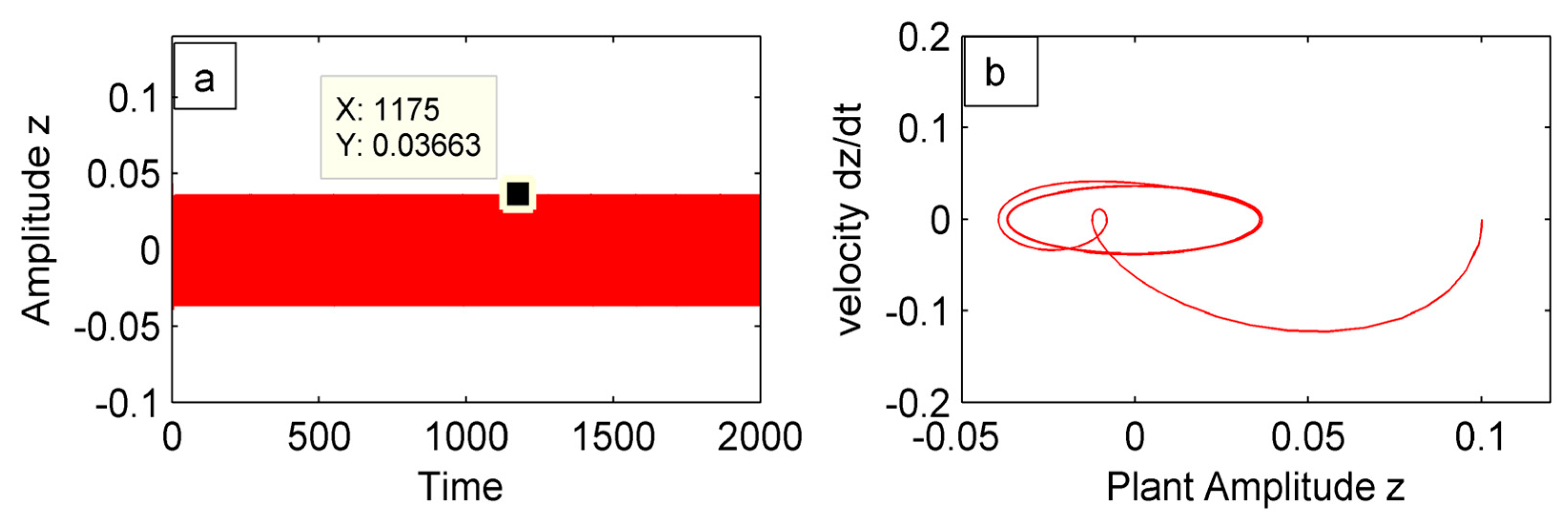
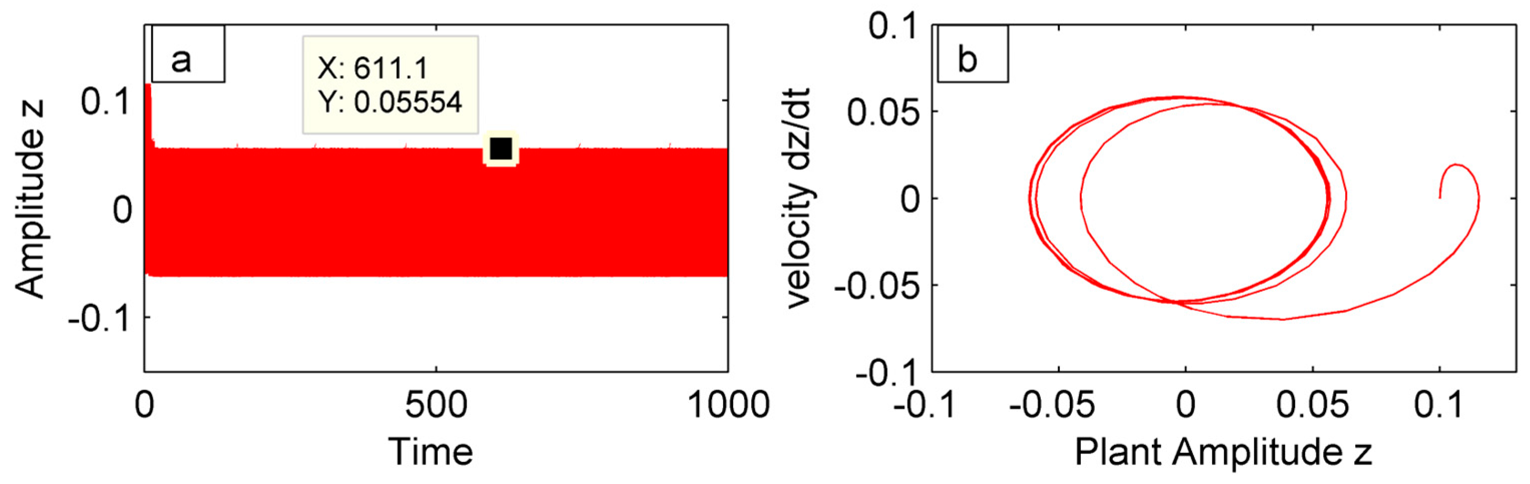
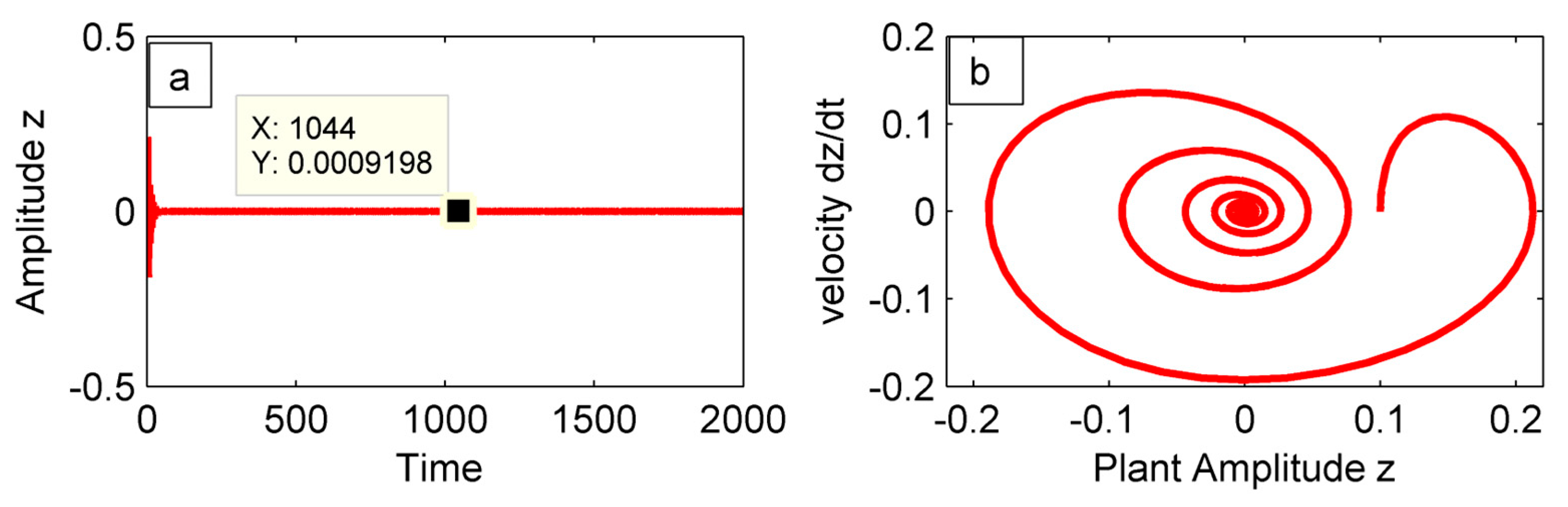
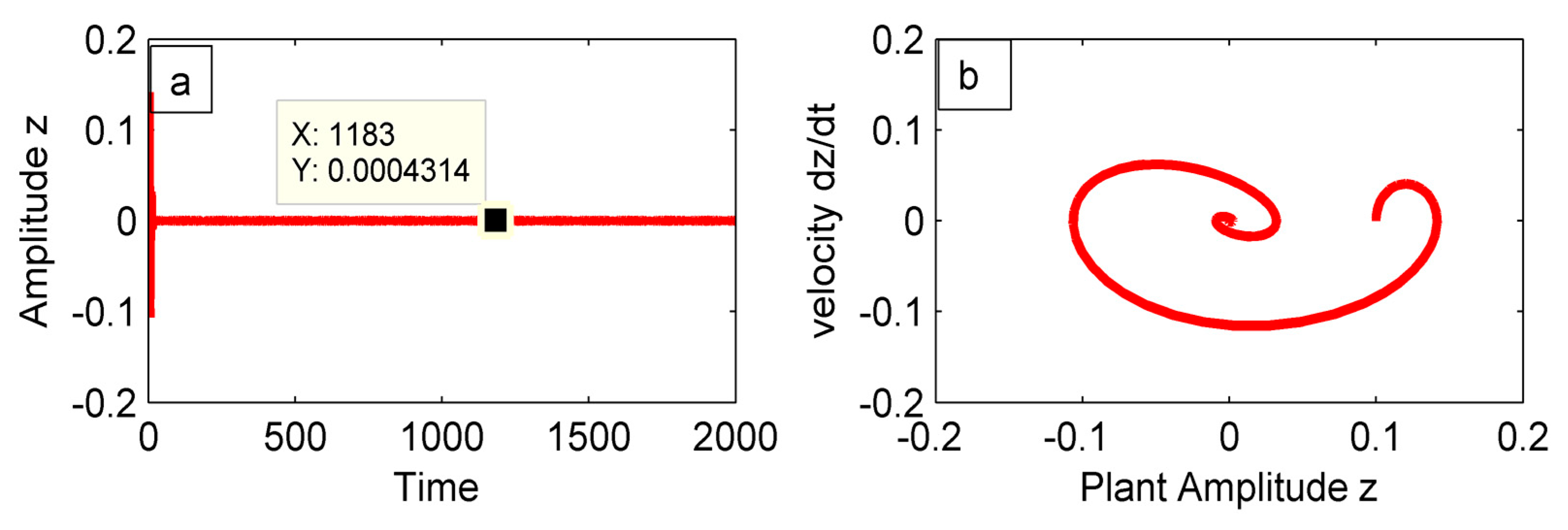
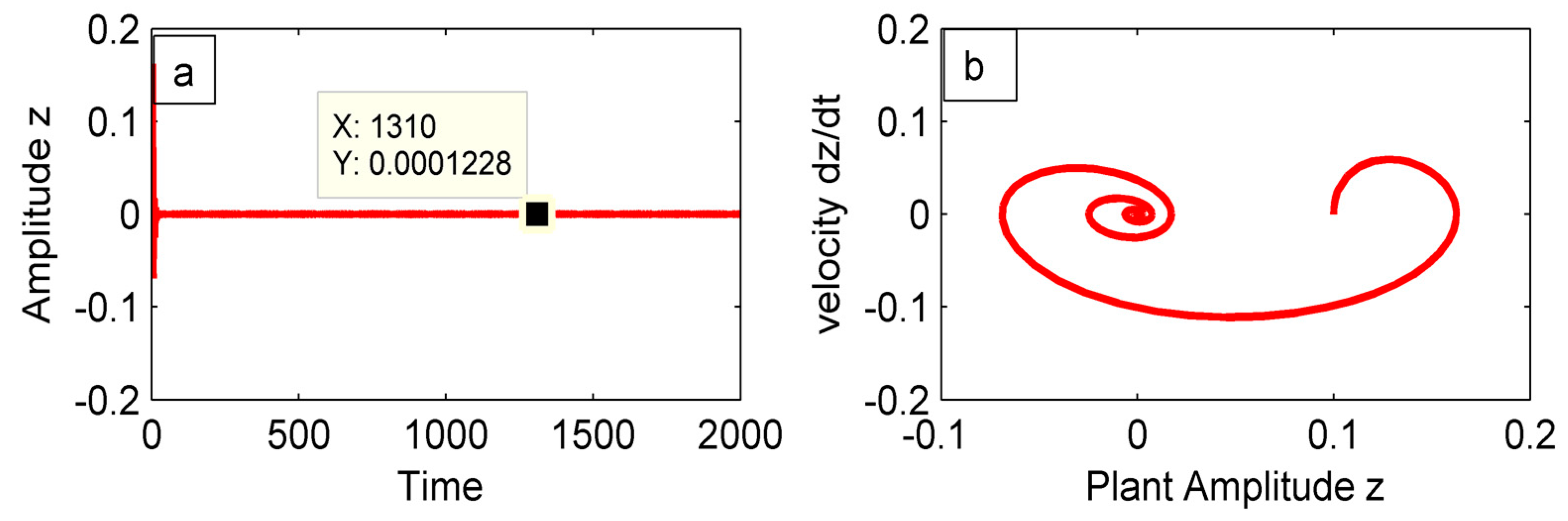
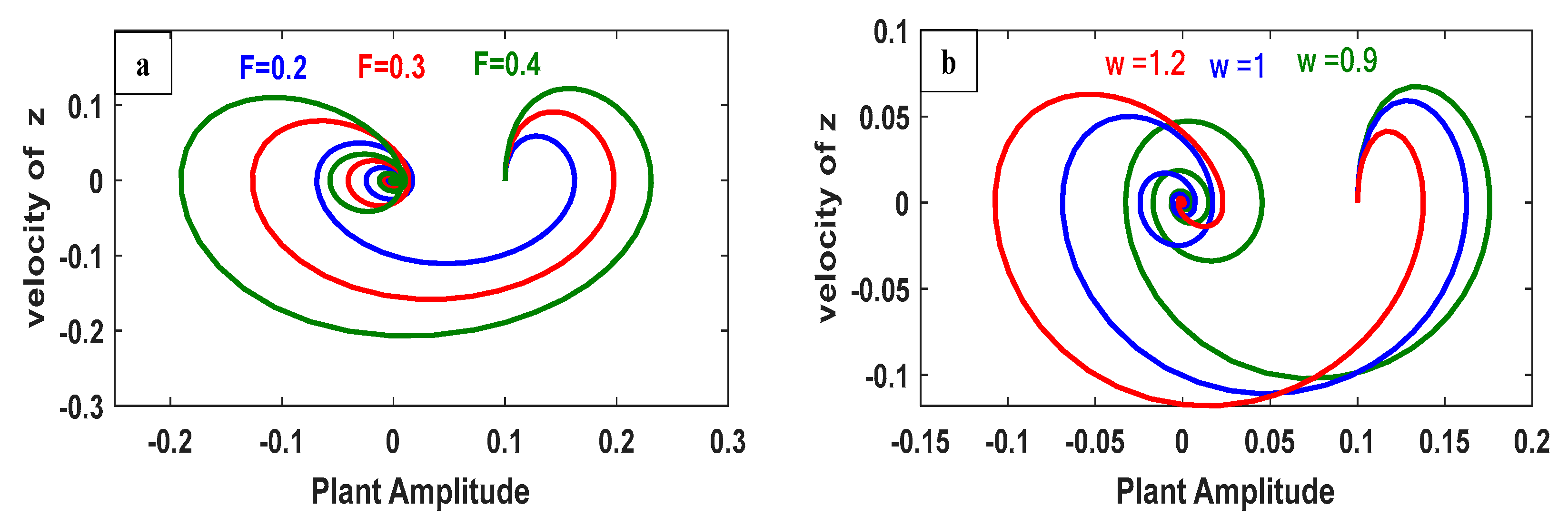
Figure 5 and Figure 6 demonstrated the system’s amplitude after two control types were added: TD and NIPPF controllers. We observed that the amplitude decreased to 0.0555 and 0.0009, respectively, indicating that the effectiveness was 55.46 and 99.27. As seen in Figure 7 and Figure 8, after IRC and NDF controllers were added, the amplitude of the system reduced until reaching 0.08 and 0.0004, and the effectiveness was 35.22 and 99.6, respectively. The ideal kind of controller for reducing the vibration of the system is a PPF controller, as illustrated in Figure 9, which reduces the vibration to 0.0001, and the effectiveness of the controller reaches 99.92%. Figure 10 illustrates a comparison of the system before and after the PPF controller was added. We examined how force affected Figure 11a, and the FR case was at its worst in Figure 11b in the phase plane. The findings indicated that, as the force increased, the velocity and displacement resonance region widened and became more at risk of vibrations and dynamic disorder, making it more difficult to regulate the system’s stability. The velocity and displacement resonance zone expanded and became fewer and larger circles as decreased.
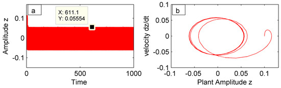
Figure 5.
(a) Time history and (b) phase plane of the system with TD at primary resonance.

Figure 6.
(a) Time history and (b) phase plane of the system with an NIPPF controller at simultaneous resonance.
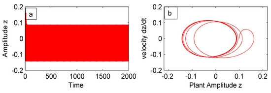
Figure 7.
(a) Time history and (b) phase plane with IRC controller at simultaneous resonance.
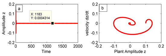
Figure 8.
(a) Time history and (b) phase plane with NDF controller at simultaneous resonance.

Figure 9.
(a) Time history and (b) phase plane of the system with a PPF controller at simultaneous resonance.
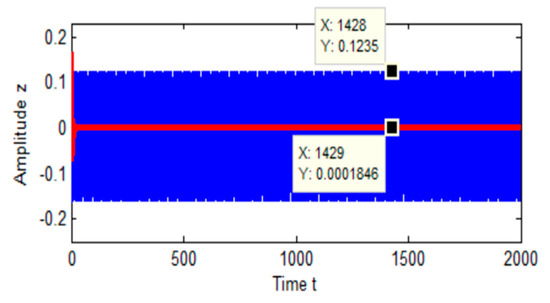
Figure 10.
Comparison of time history without control (blue curve) and after PPF control was added (red line).

Figure 11.
(a) Phase plane at different force values and (b) phase plane at different natural frequency values.
It is known that the bifurcation diagram shows how the peak values of changes as the excitation forcing frequency amplitude increases. This helps in understanding system stability and transitions between different dynamic behaviors. Based on Figure 12 and Figure 14, one can note that, for small values of , the system appears to have a single-valued response, indicating periodic motion. As increases, multiple branches emerge, indicating a transition from period-1 motion to period-doubling bifurcations. Beyond a certain threshold, the diagram becomes dense and scattered, which suggests the onset of chaotic behavior. The presence of bifurcations confirms that the system undergoes nonlinear transitions and possibly experiences resonance phenomena.
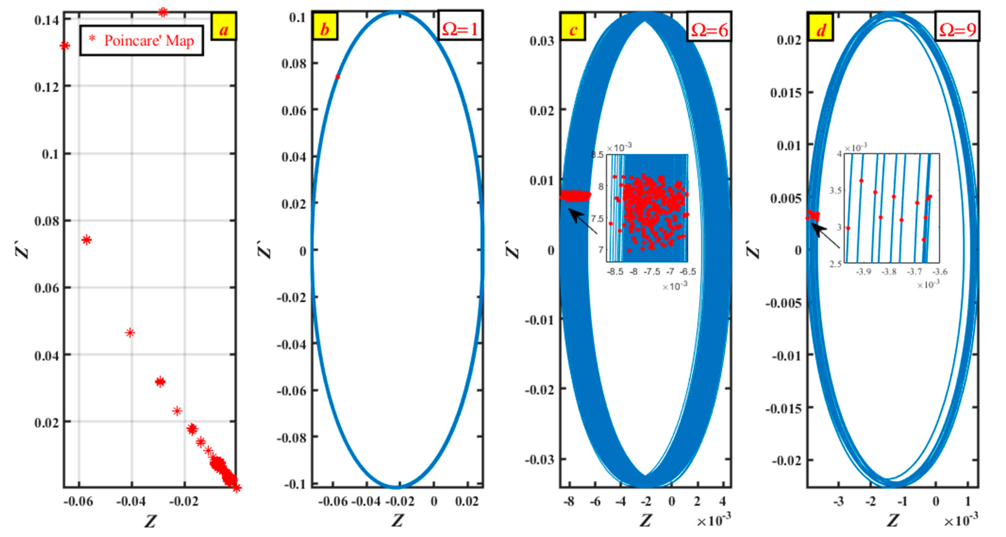
The Poincaré map drawn expresses a stroboscopic section, capturing system states without and with PPF controller at fixed intervals (here, every driving period T = (2π/ω)). It helps in identifying periodicity and chaotic behavior. The spread of points in Figure 13a and Figure 15a suggests complex behavior, possibly indicating periodic dynamics, as described in Figure 13b and Figure 15b, quasiperiodic dynamics, as described in Figure 13c and Figure 15d, or chaotic dynamics, as described in Figure 15c.

Figure 12.
Bifurcation diagram of vs. without any control.
Figure 12.
Bifurcation diagram of vs. without any control.
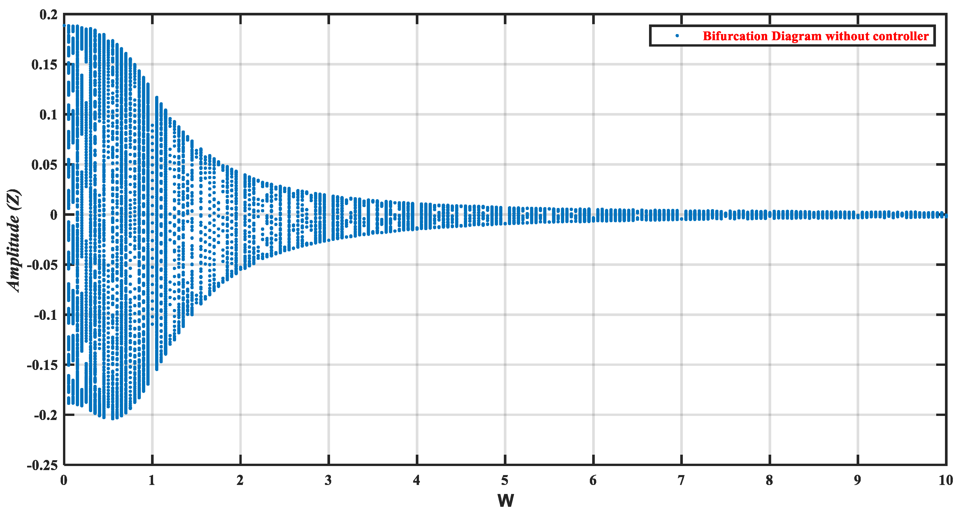

Figure 13.
(a) Poincaré maps for the system without control. (b) Phase portraits and Poincaré maps of the periodic state at . (c) Phase portraits and Poincaré maps of the quasiperiodic state at .
Figure 13.
(a) Poincaré maps for the system without control. (b) Phase portraits and Poincaré maps of the periodic state at . (c) Phase portraits and Poincaré maps of the quasiperiodic state at .
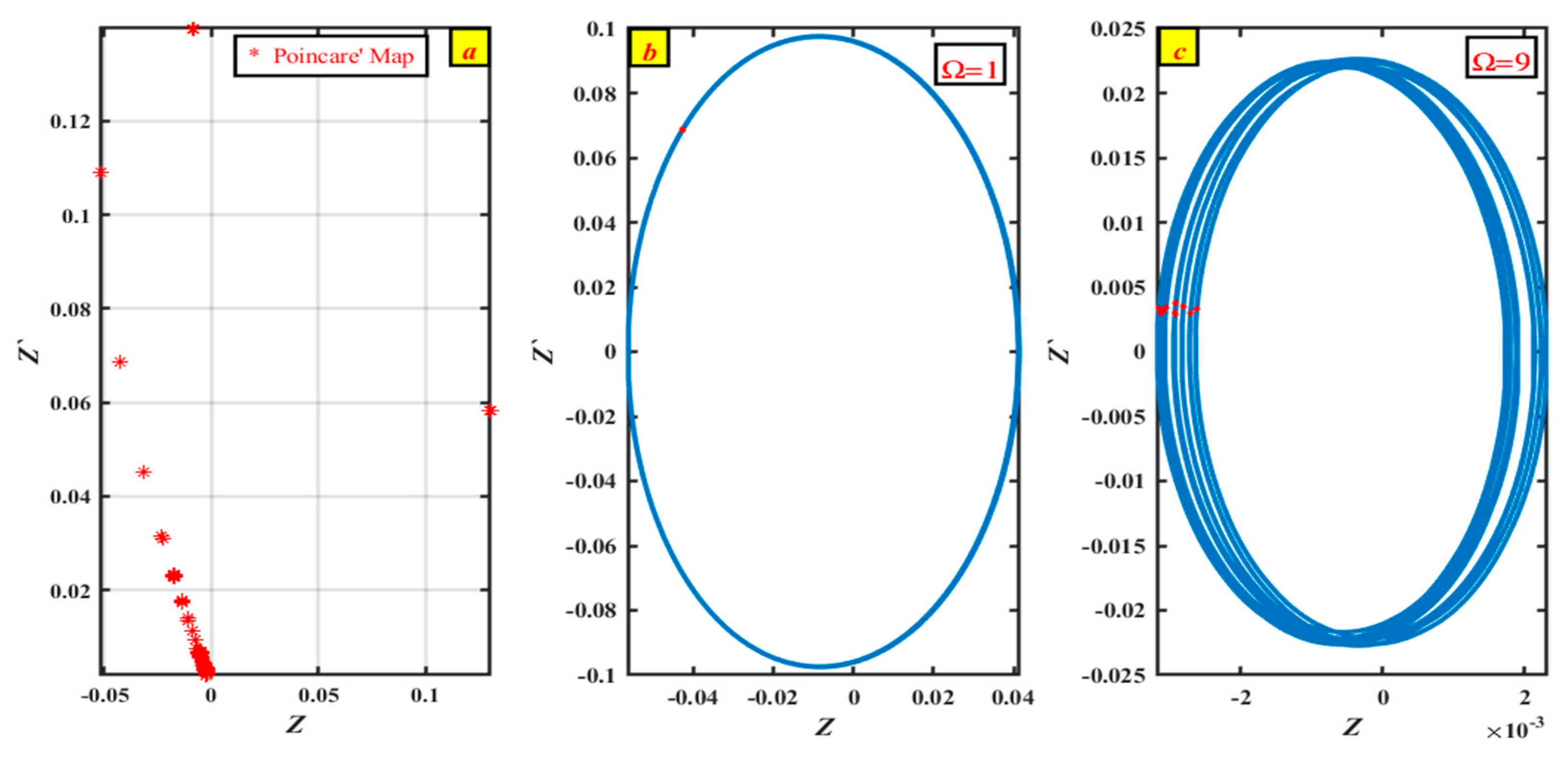

Figure 14.
Bifurcation diagram of vs. with PPF control.
Figure 14.
Bifurcation diagram of vs. with PPF control.
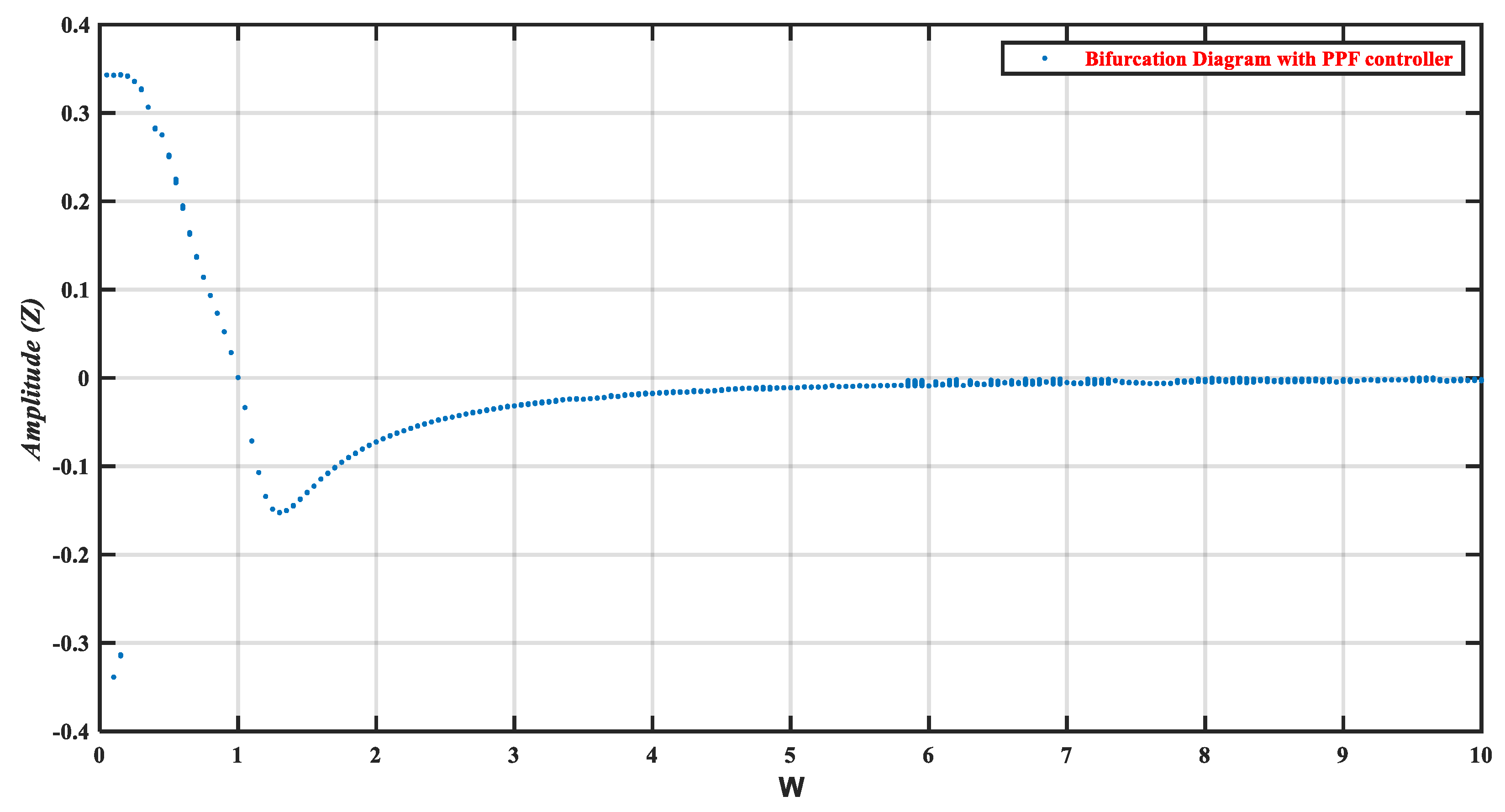
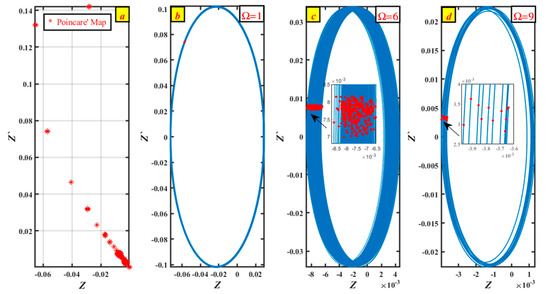
Figure 15.
(a) Poincaré maps for the system with PPF control. (b) Phase portraits and Poincaré maps of the periodic state at . (c) Phase portraits and Poincaré maps of the chaotic behavior at . (d) Phase portraits and Poincaré maps of the quasiperiodic state at .
Figure 15.
(a) Poincaré maps for the system with PPF control. (b) Phase portraits and Poincaré maps of the periodic state at . (c) Phase portraits and Poincaré maps of the chaotic behavior at . (d) Phase portraits and Poincaré maps of the quasiperiodic state at .
4.2. Frequency Response
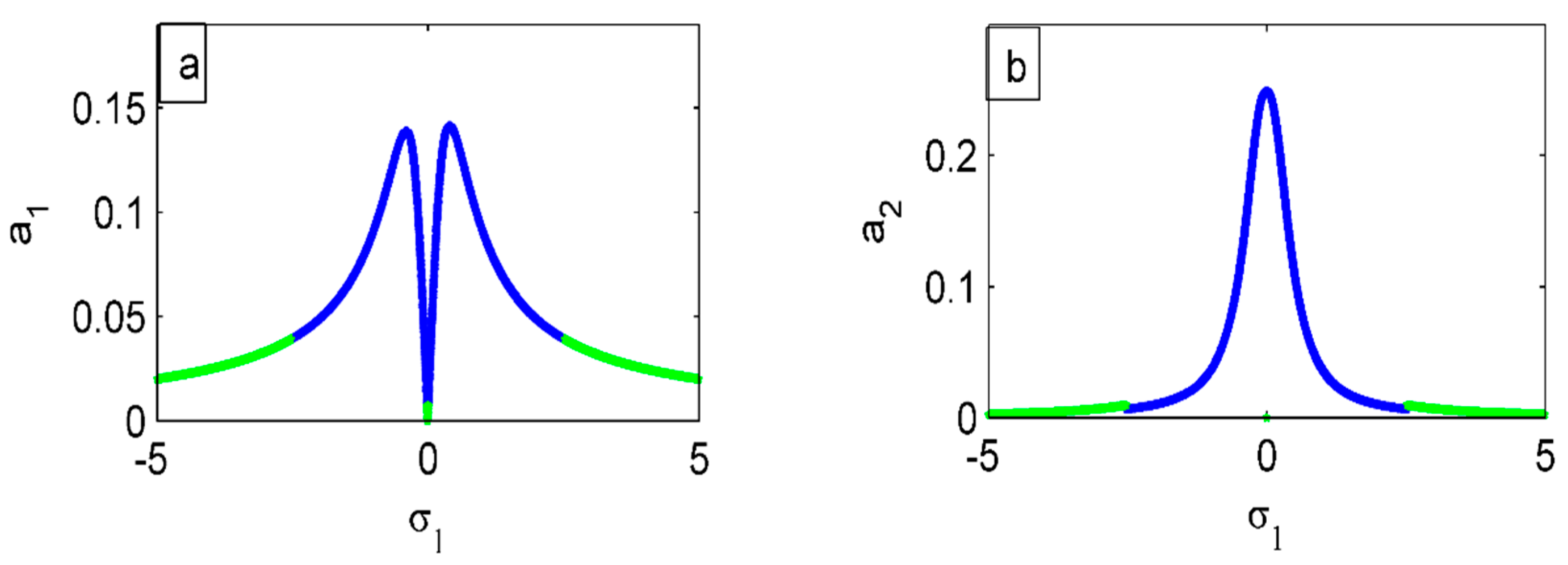
Through the use of the numerical technique, the frequency equation is graphically depicted. Equations (40)–(43) are solved numerically to obtain a graphical solution for the amplitude of the main system and PPF controller via the duetting parameter . The outcomes can be found in Figure 16, Figure 17, Figure 18, Figure 19, Figure 20, Figure 21, Figure 22, Figure 23, Figure 24, Figure 25 and Figure 26. According to the analysis of parameter value changes, the duration of stability and instability varies with various parameter values. Figure 16a shows the stability and instability of the steady-state amplitude ( against ), where the relation ( against ) is shown in Figure 16b, while the green solid line represents the unstable regions, and the other line represents stable ones. The image below demonstrates clearly that the control connection dampens lateral vibrations in the area of the bandwidth range, which is closed to . Thus, the apposition of () can best dampen the vibration.
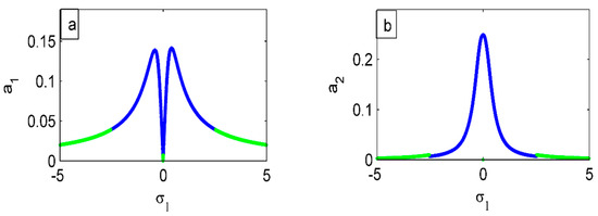
Figure 16.
FR curve of PPF controlled system at : (a) (); (b) (). (green line: unstable regions) (blue lines: stable regions).

Figure 17.
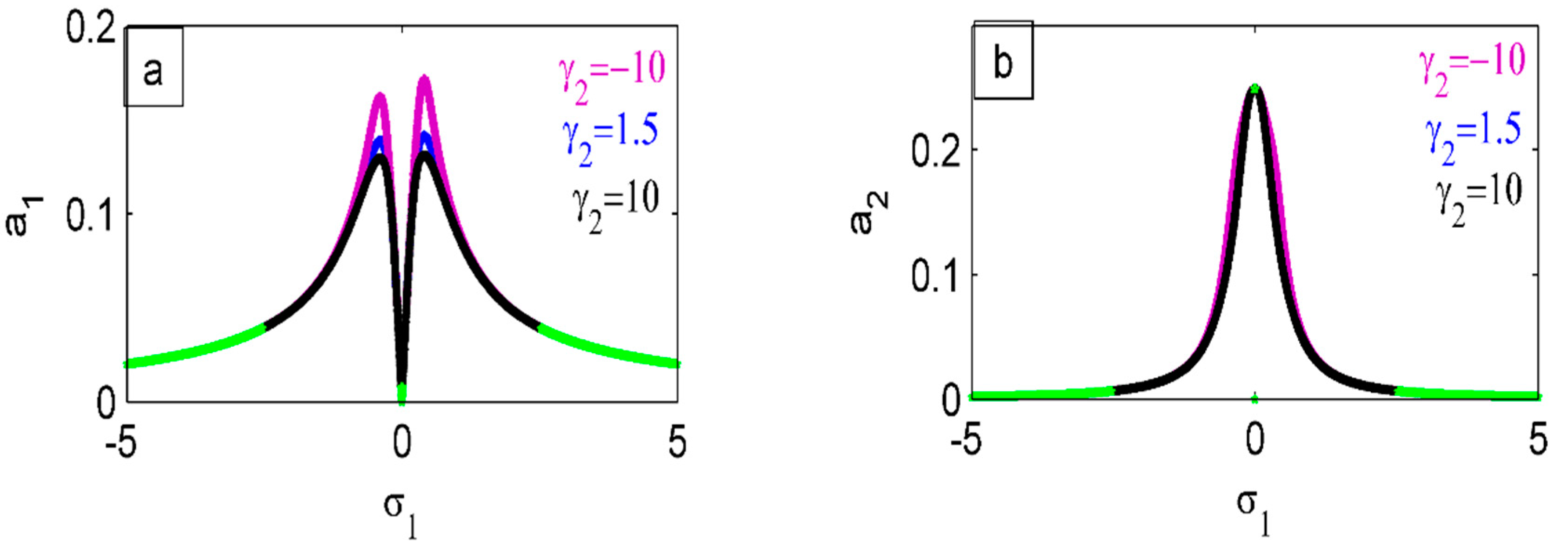
Influences of on FR curve at : (a) (); (b) ().

Figure 18.
Influences of on FR curve at : (a) (); (b) ().

Figure 19.
Influences of on FR curve at : (a) (); (b) ().

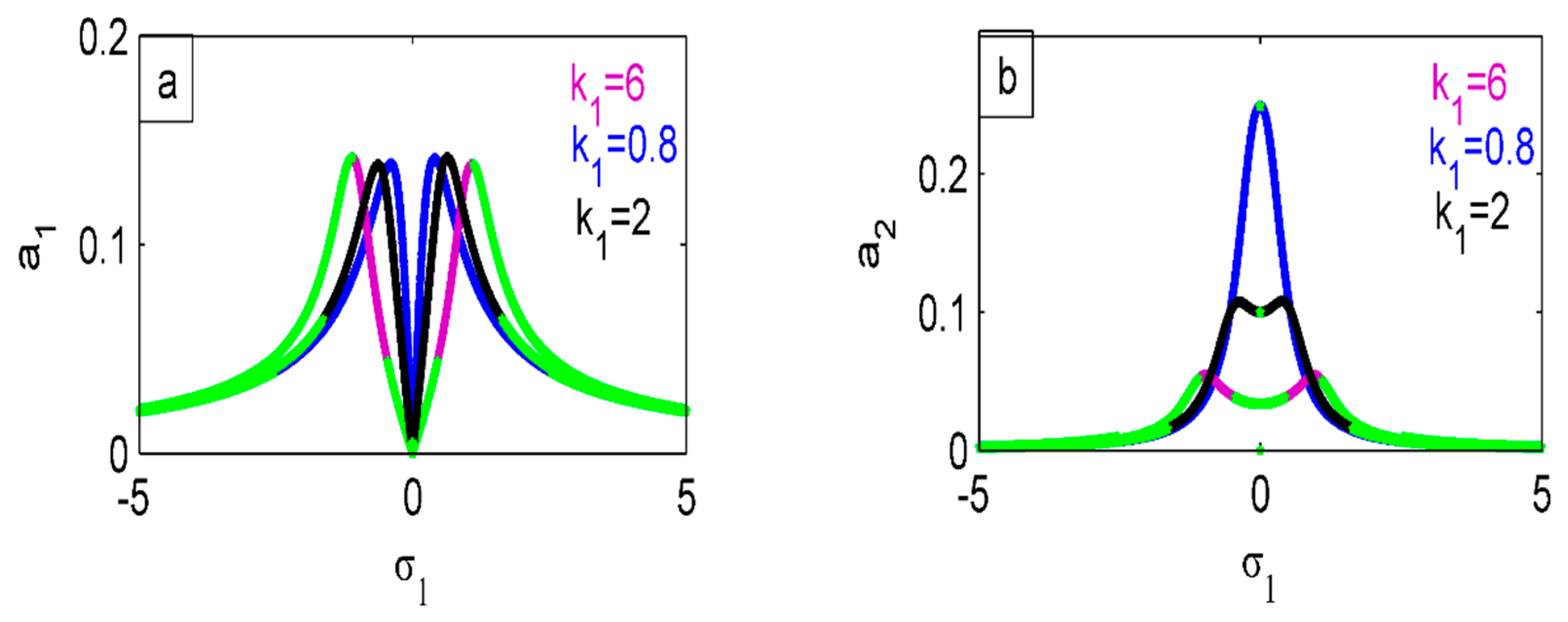
Figure 20.
Influences of on FR curve at : (a) system amplitude (–); (b) controller amplitude (–).

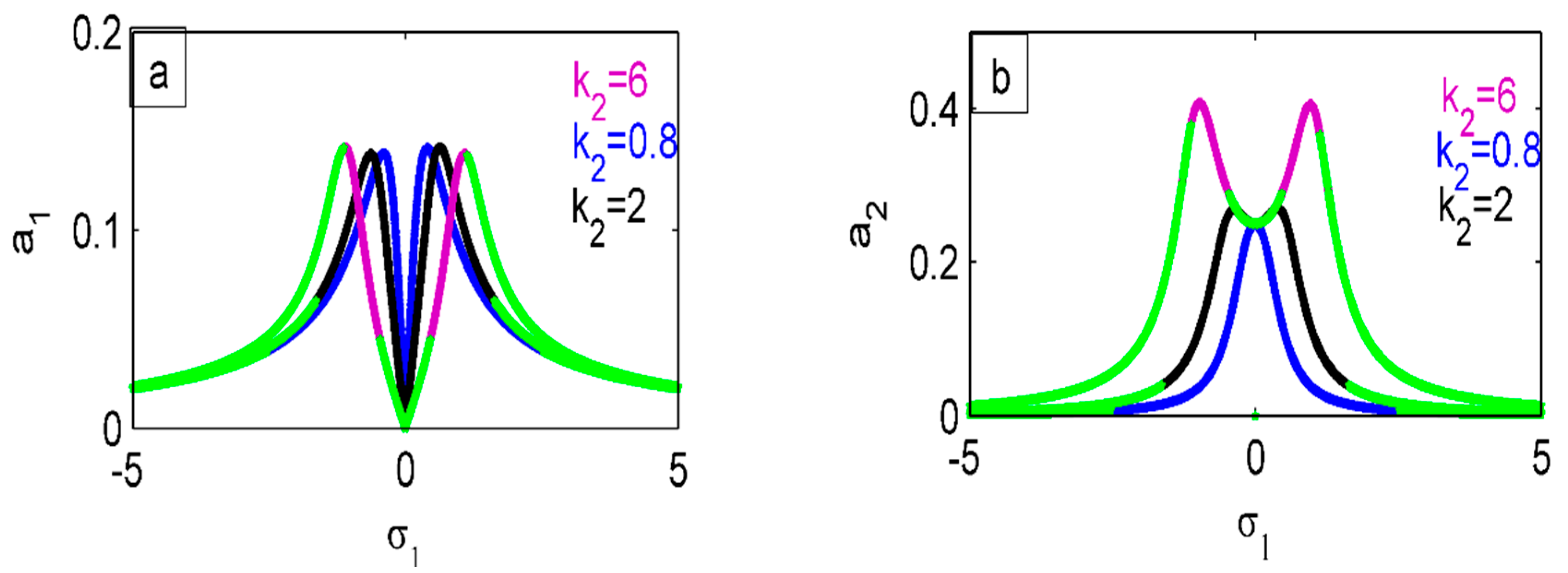
Figure 21.
Influences of on FR curve at : (a) system amplitude (–); (b) controller amplitude (–).

Figure 22.
Influences of on FR curve at : (a) system amplitude (–); (b) controller amplitude (–).
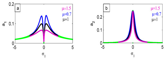
Figure 23.
Influences of on FR curve at : (a) system amplitude (–); (b) controller amplitude (–).

Figure 24.
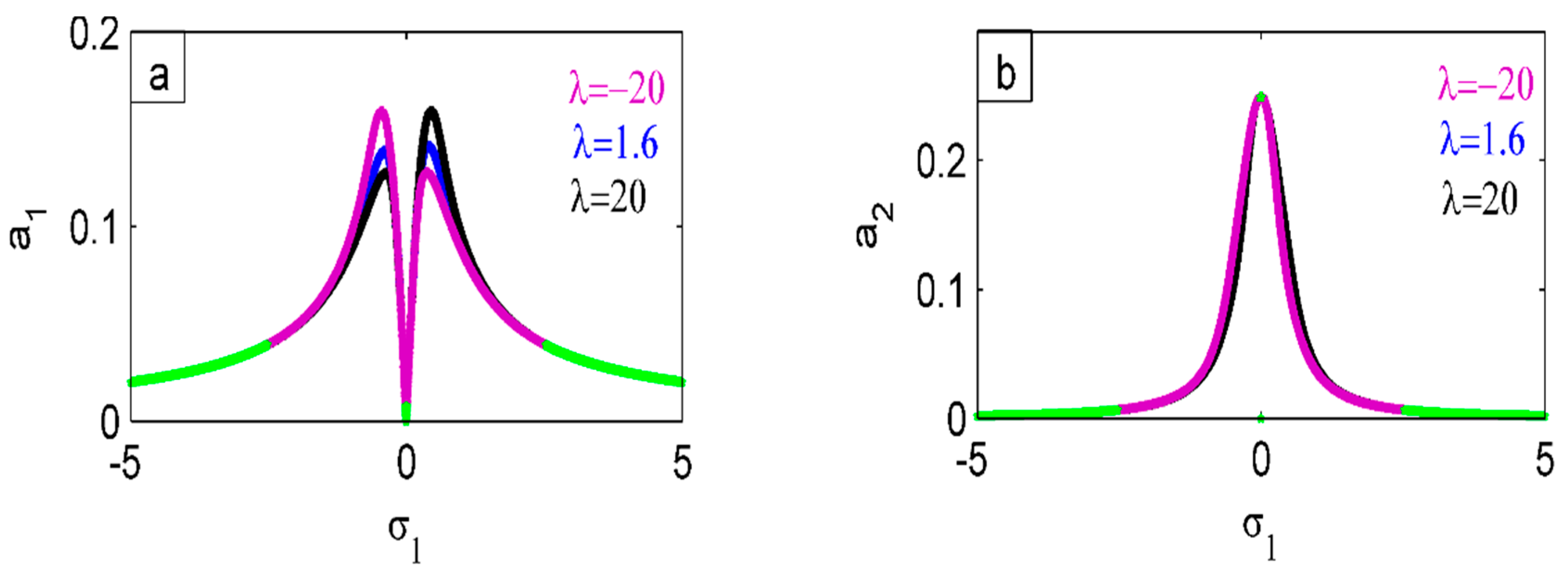
Influences of on FR curve at : (a) system amplitude (–); (b) controller amplitude (–).

Figure 25.
Influences of on FR curve at ; (a) system amplitude (–); (b) controller amplitude (–).
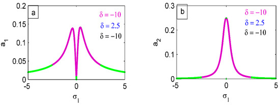
Figure 26.
Influences of on FR curve at ; (a) system amplitude (–) (b) controller amplitude (–).
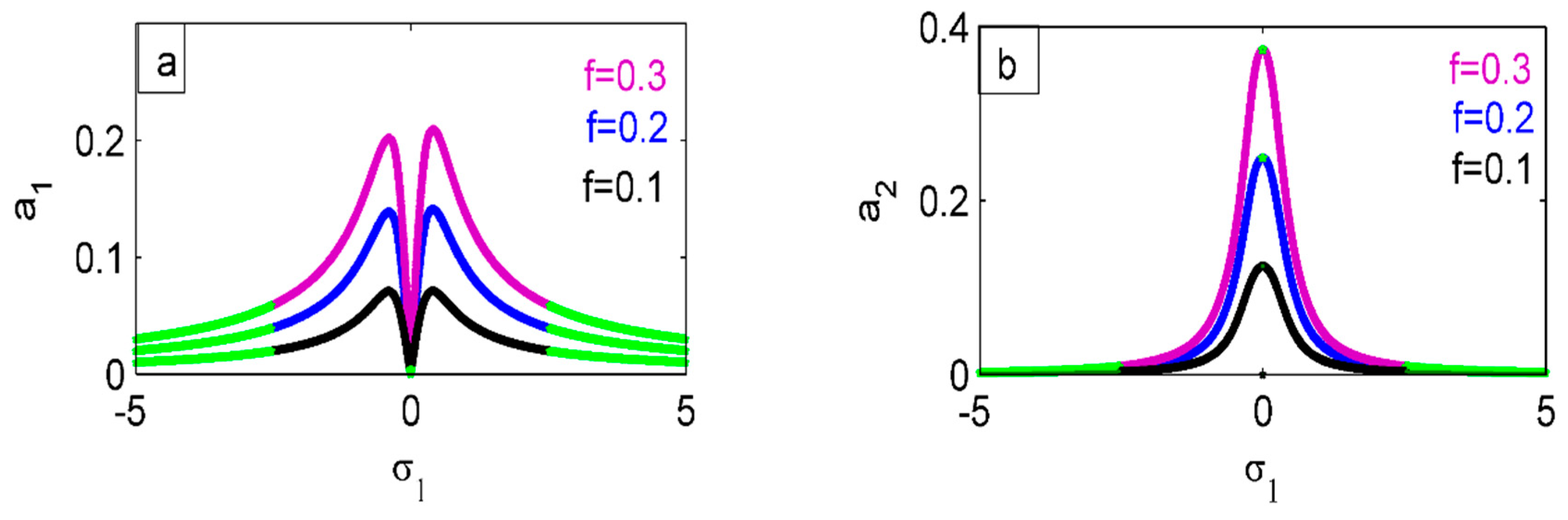
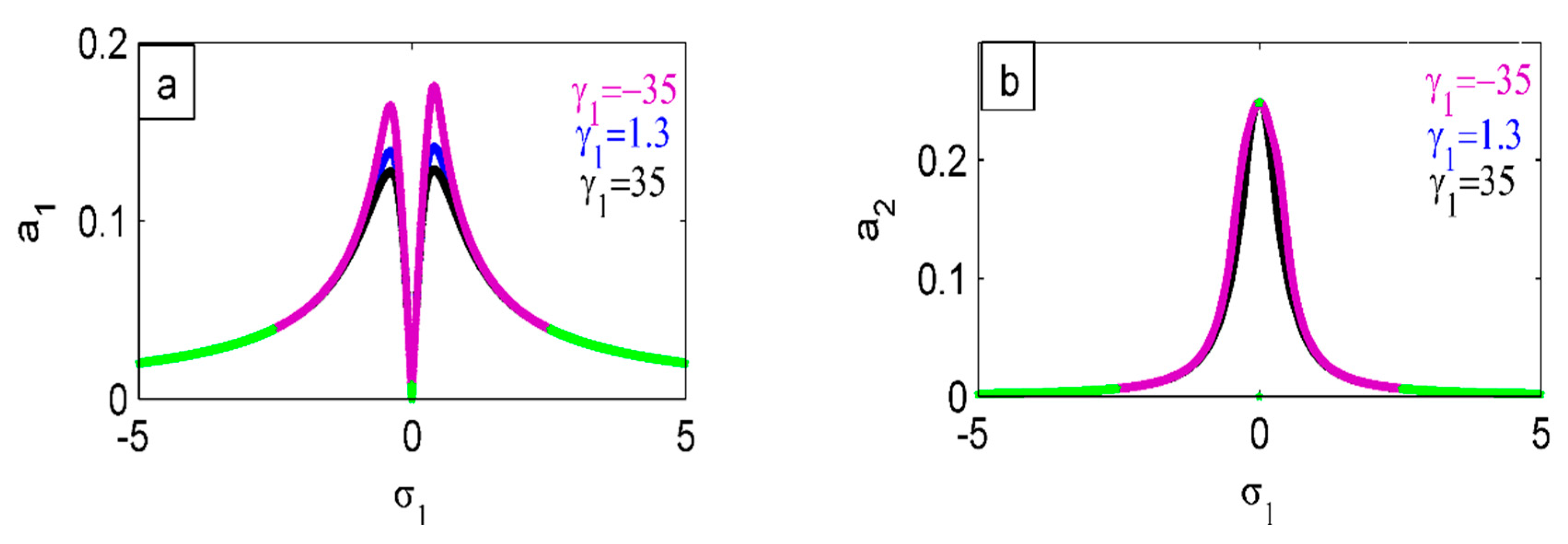
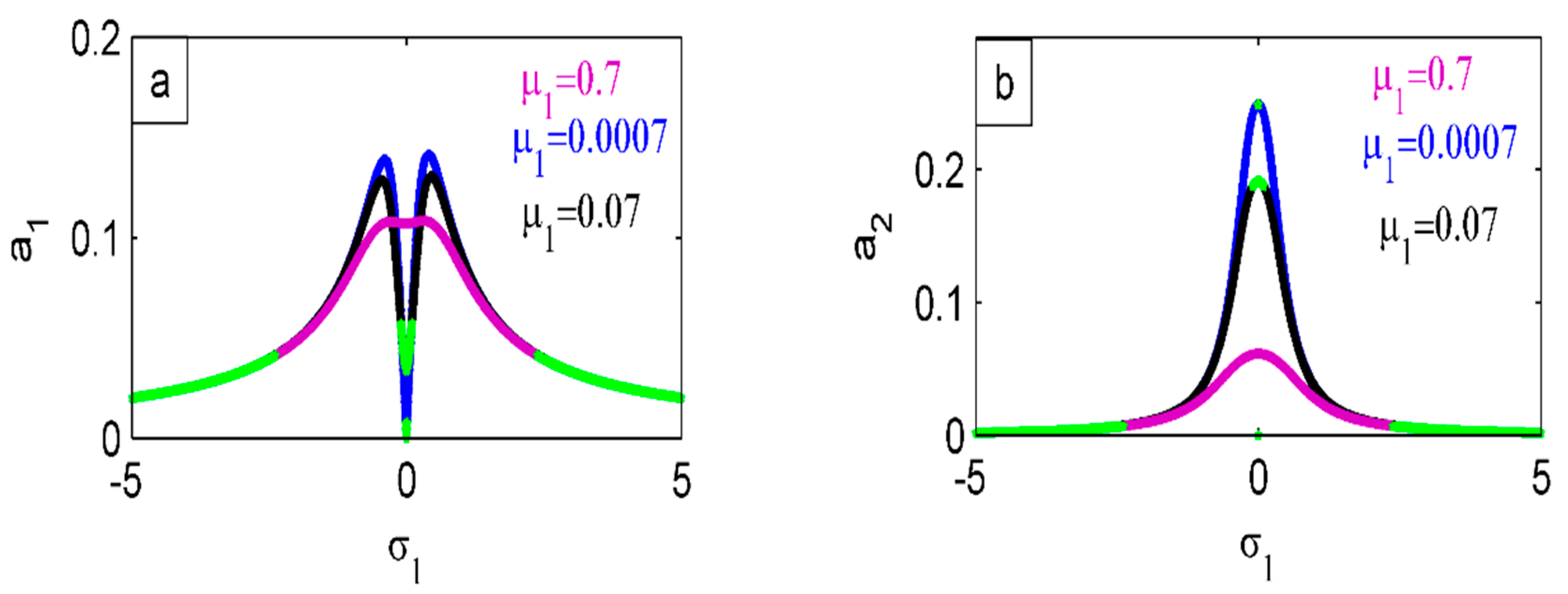
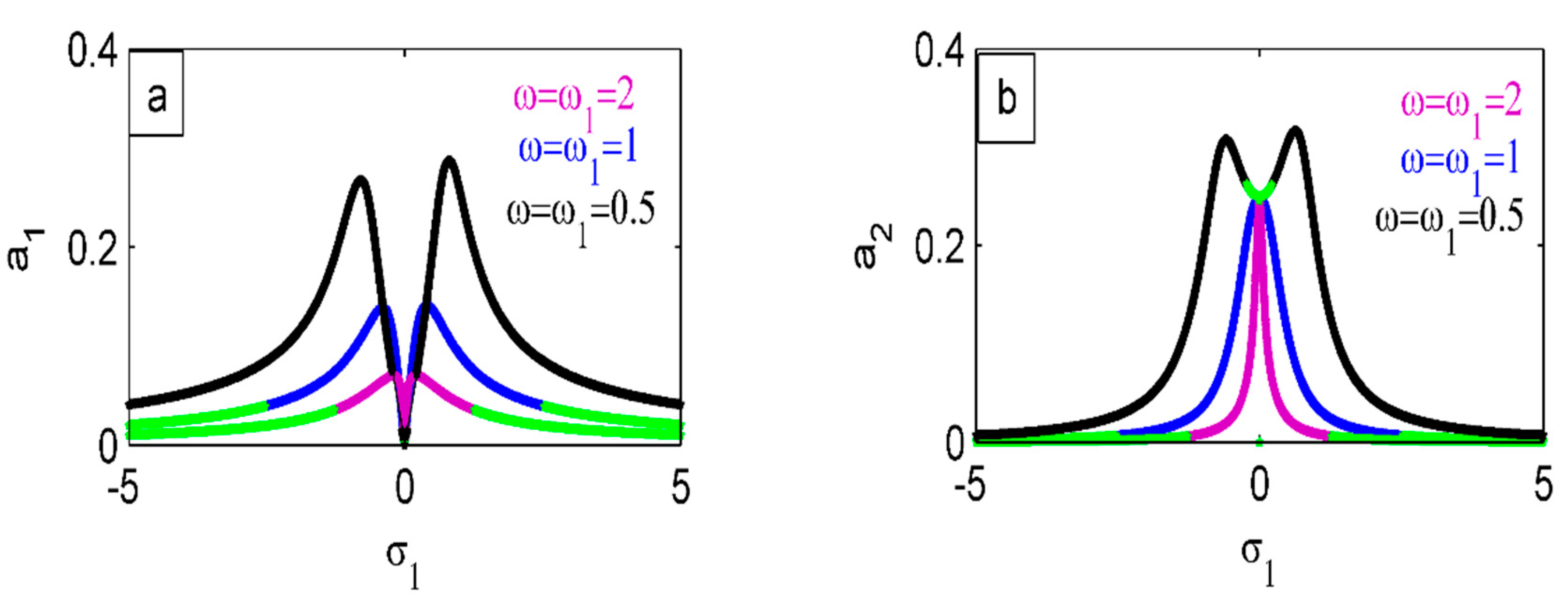
The effect of varying values on the FR curves is displayed in Figure 17. The oscillation amplitude of the system raises as grows, and the curve’s peaks rise as well, as seen in Figure 17a. As shown in Figure 17b, the beak of the curve increases for the amplitude of the control vibration as the values of increases. In Figure 18 and Figure 19, the effect of and are displayed. When smaller values of and are chosen, the two peaks of the curve from Figure 18a and Figure 19a rise, while its effect on the controller amplitude is very small, as shown in Figure 18b and Figure 19b. The effects of varying levels on the FR curve is shown in Figure 20 and Figure 21, respectively. As seen in Figure 20a and Figure 21a, accordingly, the system’s bandwidth region widens for high values of and . The controller curve’s peak splits into two peaks on either side of the bandwidth zone as values rise, as seen in Figure 20b. The effect of the parameter on the controller peaks is shown in Figure 21b. It displays that the increase in produces an increase in the controller curve’s peak expansion until it splits into two peaks on either side of the bandwidth zone, each of which rises in height. Figure 22 shows how different values of affect the FR curve. The fatness and the bandwidth of the two peaks for the structure’s curve shift to the right at small values of , as shown in Figure 22a, while there is no effect, as seen in Figure 22b.
Figure 21 illustrates how affects the FR curve. As illustrated in Figure 23a, the peaks of the system curve reduce as increases. In Figure 23b, there is no effect of on the FR curve. Figure 24 illustrates the effect of on the FR curve. As seen in Figure 24a, the two peaks of the structural curve decrease as increases, and a jump phenomenon occurs at the region where (). A small value of should be selected from this range in order to better reduce the vibrations of the structure during the resonance situation of investigation. The controller curve’s peak decreases at high values of , as shown in Figure 24b. Figure 25 shows how different values of affect the system stability and its amplitude. According to Figure 25a, the height of the system curve’s two peaks rises with small values of , but with a decreasing the value of , the peak increases until it splits into two peaks, as shown in Figure 25b. Figure 26 shows a slight effect of the parameter on the system and the controller amplitudes.
4.3. Comparison of the Time History
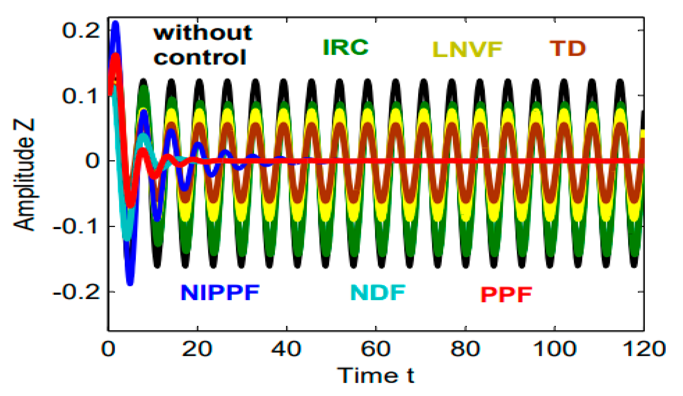
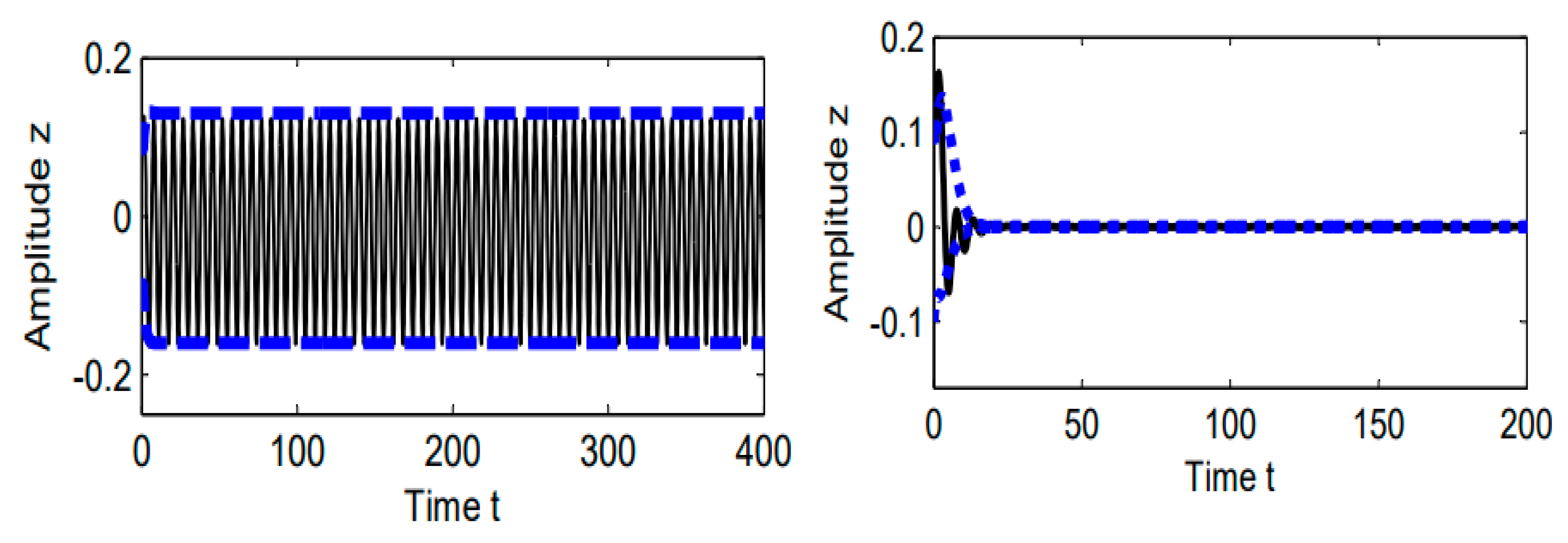
The results of the various control strategies used in the worst-case situation are displayed in Figure 27. Different types were compared so that we could choose the control that affects the system the most. In the image below, we look at LNVF, IRC, TD, NIPPF, NDF, and PPF. The outcomes showed that the PPF was the most successful technique for reducing and managing vibration. The PPF controller offers many advantages, including being insensitive to spillover, having a magnitude that rolls off quickly at high frequencies, being relatively easier to use in real-world situations, being able to ensure stability by adjusting only the structure’s stiffness properties, being cheaper than other controllers, and responding more rapidly. Figure 28 demonstrates that we were able to reach an integrated conclusion and approximately identical result by contrasting the numerical solution with the approximation solution in the worst case with and without a control.

Figure 27.
Comparison of time history between different controllers in the system.

Figure 28.
Comparison between the numerical (black line) and approximate (blue line) solution at the worst resonance case before and after the controller.
4.4. Amplitude–Frequency Curves
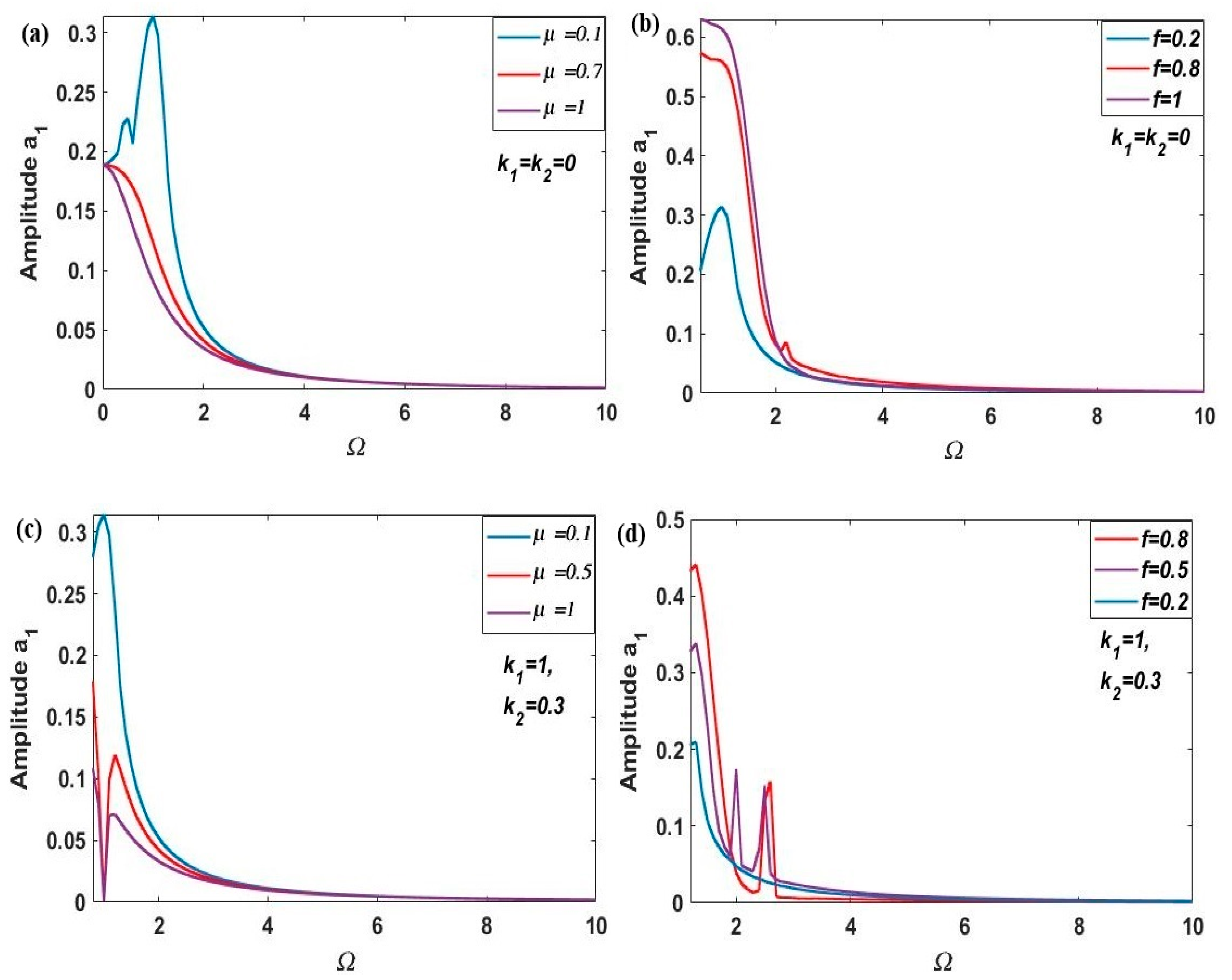
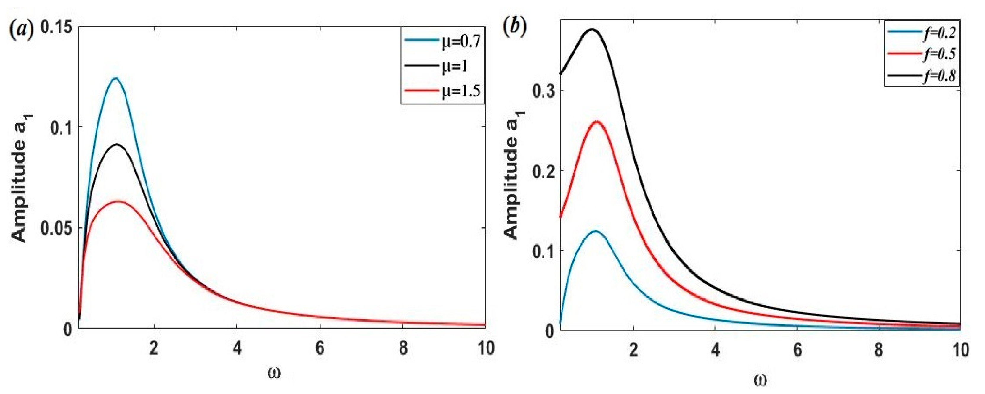
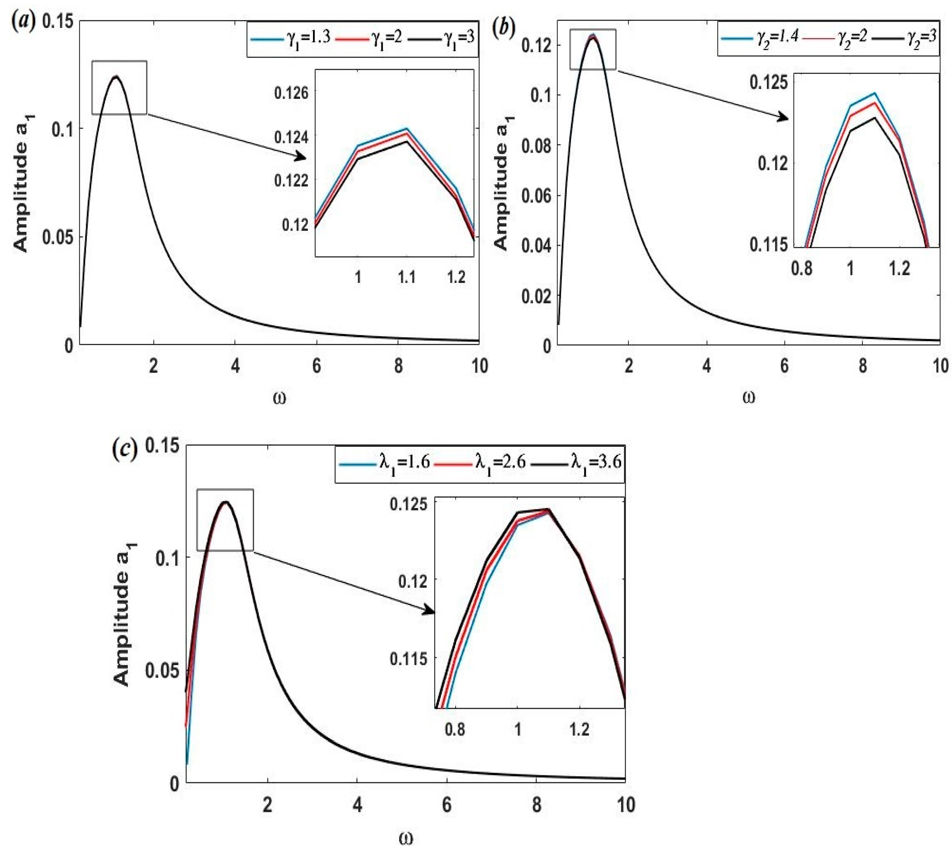
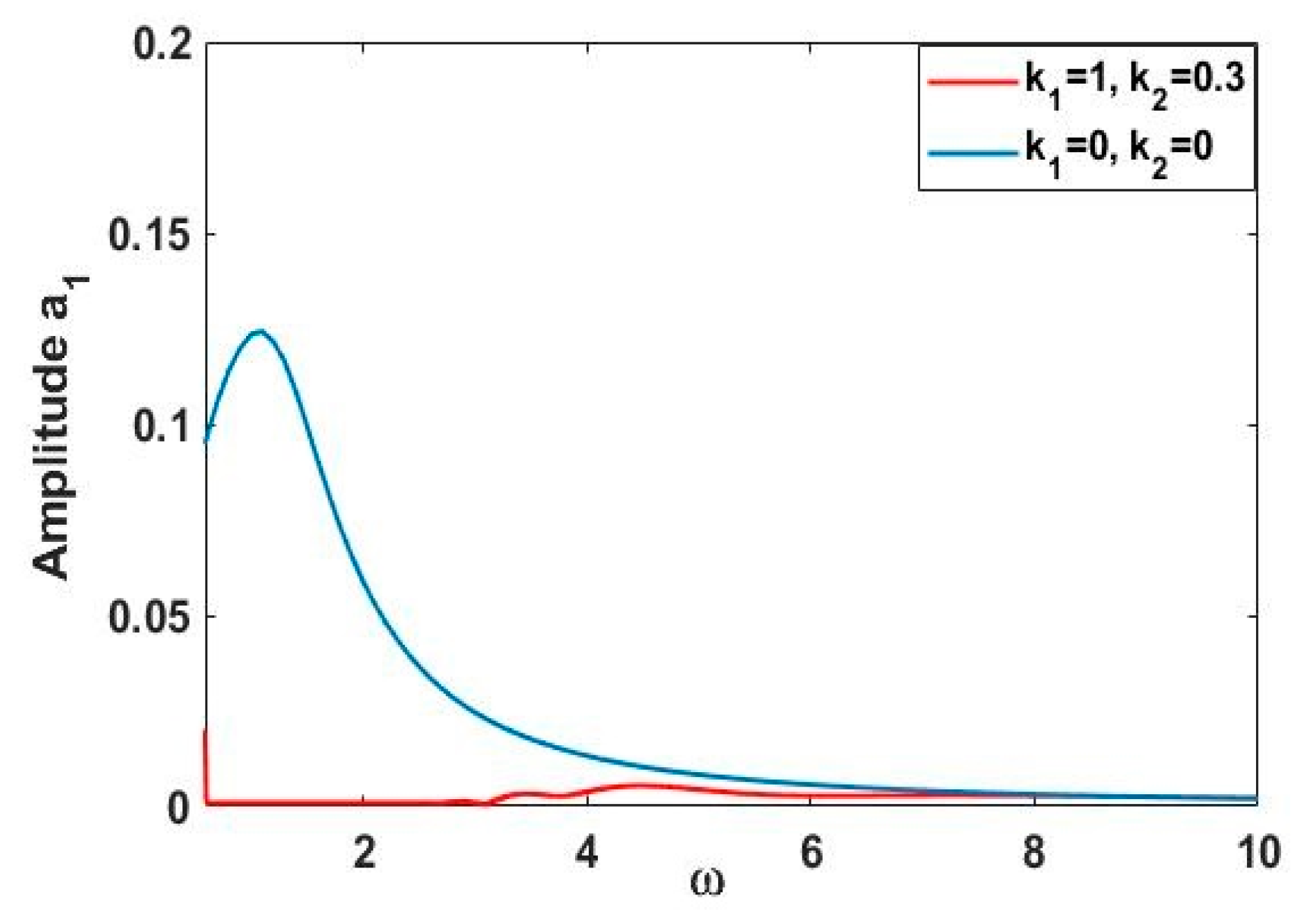
A dynamical system’s FR curve illustrates how the amplitude response of the system varies with the excitation frequency range. A cubic–quintic nonlinear hybrid oscillator’s amplitude–frequency response with external simulation and without and with insertion control, respectively, and , is shown in Figure 29 for varying values of and . Figure 29a,c shows that the system’s amplitude decreases as the damping coefficient increases, while Figure 29b,d shows that the system’s amplitude increases as the excitation amplitude increases. These findings are confirmed by the response curves in Figure 17 and Figure 23. Figure 30, Figure 31 and Figure 32 show how the internal frequency, , affects the system amplitude, . As indicated in Figure 30a,b, system amplitude decreases as the damping coefficient, , increases, and the excitation amplitude, , decreases at . The largest amplitude was found to occur at , which is also the value for the excitation frequency that produces the resonance instance. Figure 31, which displays the amplitude-internal FR for different system parameters, and settings, shows a minor system reaction as a result of changing these parameters. This finding is supported by the time history in Figure 3 and the amplitude response curves in Figure 18, Figure 19, and Figure 22. The comparison of the amplitude–FR curve without and with control is shown in Figure 32. It should be mentioned that Figure 10 supports these conclusions.

Figure 29.
Amplitude–frequency curves () in the worst resonance case and (a,b) with different values of and , respectively, before applying the control, (c,d), at different values of and , respectively, after applying the control.
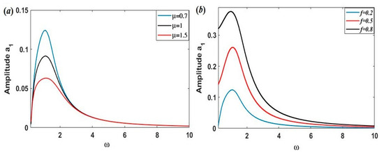
Figure 30.
Amplitude- frequency curves ( ) (a) at different values of and (b) at different values of in the worst resonance case, and .

Figure 31.
Amplitude–frequency curves () (a) at different values of , (b) at different values of , and (c) at different values of in the worst resonance case, and .
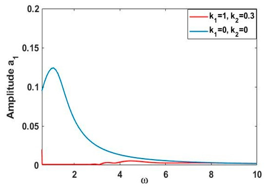
Figure 32.
Amplitude–frequency curves () before and after applying control at worst resonance case.
5. Conclusions
The goal of the current study was to examine the topic in light of the potential uses of the HRVD in a number of scientific, physics, and engineering fields. An analytically bounded solution was produced by applying the MSPT. In order to verify that the MSPT is simple to use, a graphical representation of the approximate and numerical solution was constructed. Furthermore, phase portraits were displayed, and linearized stability was reached around the HRVD’s equilibrium points. More practically, the vibration caused by an external force should be suppressed. Multi-controllers were used to suppress the vibrations that occurred in the system, and it was found that the PPF is the best controller based on its ability to suppress vibration in a shorter amount of time. The equations of motion were studied analytically, as well as numerically, which yielded the FR equations around the PR and IR 1:1 to examine the oscillator’s stability both before and after the controller was involved and the phase portrait was graphed. To find the best setting for the main system or control to increase the oscillator’s amplitude while reducing the vibration, the effects of different parameters were examined. The stability of the oscillator was determined by looking at the phase plan just before the controller was installed. Additionally, the following conclusions were reached:
- The oscillator’s amplitude was lowered to 99.92% from its pre-addition value when the PPF controller was applied, demonstrating that the PPF controller outperforms other chosen controllers, as shown in Table 1.
- The effectiveness of the PPF controller is about 1235, 137.22 when using the NIPPF controller, 308.75 when using the NDF controller, 2.24 when using the negative velocity time delay, 1.54 when using IRC, and 1.60 when using the linear velocity feedback controller.
- When the external excitation force was raised, the controlled system’s behavior increased.
- Increases in the control and feedback signal gains resulted in a large reduction in the PPF controller’s vibration frequency bandwidth.
- The damping coefficients and natural frequency had a monotonic decreasing effect on the main system’s amplitude.
- The oscillator performed best when was selected because it reduces vibrations to the point where it nearly dampens or reaches zero. Consequently, it may be stated that one of the best conditions for reducing vibrations is for the oscillators and controller’s internal resonance to equal the external resonance, or .
- A comparison of the approximate and numerical results based on time history found good comparability.
- Stability analysis was performed using the first indirect Liapunov method to classify the stable and instable ranges.
- The amplitude–frequency curves ( and ) were established to support the results obtained from the time history curves (), in addition to the response curves ().
- The phase plane diagram suggests that the system exhibits nonlinear oscillations with damping and excitation forcing frequency. The Poincaré map shows a transition from periodic to possibly chaotic behavior as the system parameters evolve. The bifurcation diagram indicates that the system undergoes bifurcations, leading to chaos as the excitation forcing frequency amplitude increases. Based on that, the system is not purely periodic or quasiperiodic, but it is also not strongly chaotic.
Author Contributions
Conceptualization, Y.A.A. and F.S.M.; methodology, A.A., Y.A.A., A.T.E.-S., F.S.M. and T.A.B.; software, T.A.B.; validation, A.A., A.T.E.-S., F.S.M. and T.A.B.; formal analysis, A.A. and F.S.M.; investigation, A.T.E.-S. and F.S.M.; resources, A.A. and Y.A.A.; data curation, A.T.E.-S., F.S.M. and T.A.B.; writing—original draft preparation, Y.A.A.; writing—review and editing, A.A., Y.A.A., A.T.E.-S., F.S.M. and T.A.B.; visualization, A.A. and Y.A.A. All authors have read and agreed to the published version of the manuscript.
Funding
This research was funded by Researchers Supporting Project number (NBU-FPEJ-2025-912-02), Northern Border University, Arar, Saudi Arabia.
Data Availability Statement
All data generated or analyzed during this study are included in this published article.
Acknowledgments
The authors extend their appreciation to the Deanship of Scientific Research at Northern Border University, Arar, KSA, for funding this research work through the project number “NBU-FPEJ-2025-912-02”.
Conflicts of Interest
The authors have not revealed any conflicting interests.
Abbreviations
| NVF | Negative velocity feedback |
| CVF | Cubic velocity feedback |
| MEs | Modulation equations |
| GM | Giant magnetostrictive |
| N/MIEMS | Nano-/Micro-electromechanical system |
| MSPT | Multiple scale perturbation technique |
| FR | Frequency response |
| RK-4 | The fourth-order Runge–Kutta procedure |
| Position, velocity, and acceleration of a hybrid oscillator system | |
| Position, velocity, and acceleration of the controller | |
| Natural frequency of the system and controller | |
| Damping coefficients | |
| Controller feedback gains | |
| Small perturbation parameter | |
| C.C | Complex conjugate |
| Des | Differential equations |
| DOF | Degree of freedom |
| HRVD | Hybrid Rayleigh–Van der Pol–Duffing oscillator |
| NIPPF | Nonlinear integral positive position feedback |
| LNVF | Linear negative velocity feedback |
| TD | Negative velocity with time delay |
| IRC | Integral resonant control |
| PPF | Positive position feedback |
| NDF | Nonlinear derivative feedback |
| PR | Primary resonance |
| IR | Internal resonance |
| SR | Simultaneous resonance |
| Amplitude before control | |
| Amplitude after control |
Appendix A
Appendix B
The positive position feedback (PPF) controller is a control strategy that adds a feedback term proportional to the position of the system to improve the damping and response characteristics. The PPF controller helps the system return to equilibrium faster and with less oscillation by effectively increasing the system’s damping:
Here, is the feedback gain. This term attempts to reach the system’s equilibrium point when the position deviates, leading to increased damping in the system and faster stabilization. PPF is one of the most used controllers in the field of active vibration control; consider the system as described by a single degree of freedom, as indicated by the following equation:
The PPF controller is implemented using a second-order dynamic system defined as
where and are the damping and frequency, respectively, and is the gain.
References
- Anjum, N.; He, J.H. Nonlinear dynamic analysis of vibratory behavior of a graphene nano/microelectromechanical system. Math. Methods Appl. Sci. 2020, 1–16. [Google Scholar] [CrossRef]
- Skrzypacz, P.; He, J.H.; Ellis, G.; Kuanyshbay, M. A Simple approximation of periodic solutions to microelectromechanical system model of oscillating parallel plate capacitor. Math. Methods Appl. Sci. 2020, 1–8. [Google Scholar] [CrossRef]
- Anjum, N.; He, J.H. Higher-order homotopy perturbation method for conservative nonlinear oscillators generally and microelectromechanical systems’ oscillators particularly. Int. J. Mod. Phys. B 2020, 34, 2050313. [Google Scholar] [CrossRef]
- He, J.H.; Skrzypacz, P.S.; Zhang, Y.; Pang, J. Approximate periodic solutions to microelectromechanical system oscillator subject to magnetostatic excitation. Math. Methods Appl. Sci. 2020, 1–8. [Google Scholar] [CrossRef]
- Anjum, N.; He, J.H. Homotopy perturbation method for N/MEMS oscillators. Math. Methods Appl. Sci. 2020, 1–15. [Google Scholar] [CrossRef]
- He, J.H.; El-Dib, Y.O. Periodic property of the time-fractional Kundu-Mukherjee-Naskar equation. Results Phys. 2020, 19, 103345. [Google Scholar] [CrossRef]
- He, C.H.; Liu, C.; He, J.H.; Gepreel, K.A. Low frequency property of a fractal vibration model for a concrete beam. Fractals 2021, 29, 2150117. [Google Scholar] [CrossRef]
- He, J.H.; Kou, S.J.; He, C.H.; Zhang, Z.W.; Gepreel, K.A. Fractal oscillation and its frequency-amplitude property. Fractals 2021, 29, 2150105. [Google Scholar] [CrossRef]
- Ueda, Y. Randomly transitional phenomena in the system governed by Dufng’s equation. J. Stat. Phys. 1979, 20, 181–196. [Google Scholar] [CrossRef]
- Nayfeh, A.H.; Chin, C.M.; Pratt, J. Perturbation methods in nonlinear dynamics applications to machining dynamics. J. Manuf. Sci. Eng. 1997, 119, 485–493. [Google Scholar] [CrossRef]
- Mickens, R.E. Oscillations in Planar Dynamic Systems; World Scientifc: Singapore, 1996. [Google Scholar]
- Moatimid, G.M. Stability analysis of a parametric Dufng oscillator. J. Eng. Mech. 2020, 146, 05020001. [Google Scholar] [CrossRef]
- Ghaleb, A.F.; Abou-Dina, M.S.; Moatimid, G.M.; Zekry, M.H. Analytic approximate solutions of the cubic-quintic Dufng-van der Pol equation with two-external periodic forcing terms: Stability analysis. Math. Comput. Simul. 2021, 180, 129–151. [Google Scholar] [CrossRef]
- Russell, D.; Fleming, A.J.; Aphale, S.S. Improving the positioning bandwidth of the Integral Resonant Control Scheme through strategic zero placement. IFAC Proc. Vol. 2014, 47, 6539–6544. [Google Scholar] [CrossRef]
- Cveticanin, L.; Abd El-Latif, G.M.; El-Naggar, A.M.; Ismail, G.M. Periodic solution of the generalized Rayleigh equation. J. Sound Vib. 2008, 318, 580–591. [Google Scholar] [CrossRef]
- Hill, T.L.; Neild, S.A.; Wagg, D.J. Comparing the direct normal form method with harmonic balance and the method of multiple scales. Procedia Eng. 2017, 199, 869–874. [Google Scholar] [CrossRef]
- Huang, C.; Li, H.; Cao, J. A novel strategy of bifurcation control for a delayed fractional predator-prey model. Appl. Math. Comput. 2019, 347, 808–838. [Google Scholar] [CrossRef]
- Barron, M.A. Stability of a ring of coupled van der Pol oscillators with non-uniform distribution of the coupling parameter. J. Appl. Res. Technol. 2016, 14, 62–66. [Google Scholar] [CrossRef]
- Miwadinou, C.H.; Monwanou, A.V.; Yovogan, J.; Hinvi, L.A.; Tuwa, P.N.; Orou, J.C. Modeling nonlinear dissipative chemical dynamics by a forced modifed Van der Pol-Dufng oscillator with asymmetric potential: Chaotic behaviors predictions. Chin. J. Phys. 2018, 56, 1089–1104. [Google Scholar] [CrossRef]
- Wang, W.; Wang, X.; Hua, X.; Song, G.; Chen, Z. Vibration control of vortex-induced vibrations of a bridge deck by a single-side pounding tuned mass damper. Eng. Struct. 2018, 173, 61–75. [Google Scholar] [CrossRef]
- Syed, H.H. Comparative study between positive position feedback and negative derivative feedback for vibration control of a flexible arm featuring piezoelectric actuator. Int. J. Adv. Robot. Syst. 2017, 14, 1729881417718801. [Google Scholar] [CrossRef]
- Moatimid, G.M.; EL-Sayed, A.T.; Salman, H.F. Different controllers for suppressing oscillations of a hybrid oscillator via non-perturbative analysis. Sci. Rep. 2024, 14, 307. [Google Scholar] [CrossRef]
- Jung, W.; Noh, I.; Kang, D. The vibration controller design using positive position feedback control. In Proceedings of the 2013 13th International Conference on Control, Automation and Systems (ICCAS 2013), Gwangju, Republic of Korea, 20–23 October 2013; IEEE: Piscataway, NJ, USA, 2013; pp. 1721–1724. [Google Scholar]
- El-Ganaini, W.A.; Saeed, N.A.; Eissa, M. Positive position feedback (PPF) controller for suppression of nonlinear system vibration. Nonlinear Dyn. 2013, 72, 517–537. [Google Scholar] [CrossRef]
- Omidi, E.; Mahmoodi, S.N. Sensitivity analysis of the nonlinear integral positive position feedback and integral resonant controllers on vibration suppression of nonlinear oscillatory systems. Commun. Nonlinear Sci. Numer. Simul. 2015, 22, 149–166. [Google Scholar] [CrossRef]
- Kandil, A.; El-Gohary, H. Investigating the performance of a time delayed proportional derivative controller for rotating blade vibrations. Nonlinear Dyn. 2018, 91, 2631–2649. [Google Scholar] [CrossRef]
- Nayfeh, A.H. Problems in Perturbation; Wiley: New York, NY, USA, 1985. [Google Scholar]
- Bauomy, H.S.; EL-Sayed, A.T.; El-Bahrawy, F.T. Integral resonant negative derivative feedback suppression control strategy for nonlinear dynamic vibration behavior model. Chaos Solitons Fractals 2024, 189, 115686. [Google Scholar] [CrossRef]
- Amer, T.S.; Bahnasy, T.A.; Abosheiaha, H.F.; Elameer, A.S.; Almahalawy, A. The stability analysis of a dynamical system equipped with a piezoelectric energy harvester device near resonance. J. Low Freq. Noise Vib. Act. Control. 2024. [Google Scholar] [CrossRef]
- Amer, Y.A.; Bahnasy, T.A.; Almahalawy, A. Vibration analysis of permanent magnet motor rotor system in shearer semi-direct drive cutting unite with speed controller and multi-excitation forces. Appl. Math. Inf. Sci. 2021, 15, 373–381. [Google Scholar]
- Bauomy, H.S.; EL-Sayed, A.T.; Amer, T.S.; Abohamer, M.K. Negative derivative feedback control and bifurcation in a two-degree-of-freedom coupled dynamical system. Chaos Solitons Fractals 2025, 193, 116138. [Google Scholar] [CrossRef]
- Kumar, P.; Kumar, A.; Racic, V.; Erlicher, S. Modelling vertical human walking forces using self-sustained oscillator. Mech. Syst. Signal Process 2018, 99, 345–363. [Google Scholar] [CrossRef]
- Nayfeh, A.H.; Mook, D.T. Nonlinear Oscillations; John Wiley and Sons: New York, NY, USA, 2008. [Google Scholar]


Disclaimer/Publisher’s Note: The statements, opinions and data contained in all publications are solely those of the individual author(s) and contributor(s) and not of MDPI and/or the editor(s). MDPI and/or the editor(s) disclaim responsibility for any injury to people or property resulting from any ideas, methods, instructions or products referred to in the content. |
© 2025 by the authors. Licensee MDPI, Basel, Switzerland. This article is an open access article distributed under the terms and conditions of the Creative Commons Attribution (CC BY) license (https://creativecommons.org/licenses/by/4.0/).