Article

Applied Mathematical Techniques for the Stability and Solution of Hybrid Fractional Differential Systems

by
Mohammad Alakel Abazid
1,*,
Muath Awadalla
1,
Murugesan Manigandan
2,3,* and
Jihan Alahmadi
4
1
Department of Mathematics and Statistics, College of Science, King Faisal University, Hofuf 31982, Saudi Arabia
2
Center for Nonlinear and Complex Networks, SRM TRP Engineering College, Tiruchirapalli 621 105, India
3
Center for Research, Easwari Engineering College, Chennai 600 089, India
4
Department of Mathematics, College of Science and Humanities in Al-Kharj, Prince Sattam Bin Abdulaziz University, Al-Kharj 11942, Saudi Arabia
*
Authors to whom correspondence should be addressed.
Mathematics 2025, 13(6), 941; https://doi.org/10.3390/math13060941
Submission received: 27 February 2025 / Revised: 7 March 2025 / Accepted: 11 March 2025 / Published: 12 March 2025

Abstract

:
This paper addresses a coupled system of hybrid fractional differential equations governed by non-local Hadamard-type boundary conditions. The study focuses on proving the existence, uniqueness, and stability of the system’s solutions. To achieve this, we apply Banach’s fixed point theorem and the Leray–Schauder alternative, while the stability is verified through the Ulam–Hyers framework. Additionally, a numerical example is presented to illustrate the practical relevance of the theoretical findings.
MSC:
34A08; 26a33; 34K37

1. Introduction

Fractional differential equations (FDEs) and systems of fractional differential equations have gained significant attention in applied sciences due to their capability to model certain complex dynamical systems more effectively than classical integer-order models, particularly those involving memory effects and hereditary properties. These equations incorporate non-locality and memory effects, making them highly applicable in diverse fields such as control theory, viscoelasticity, bioengineering, signal processing, and fluid dynamics. The generalization of differentiation to non-integer orders allows for a more flexible representation of real-world phenomena. Researchers utilize FDEs to analyze anomalous diffusion, population dynamics, and electrical circuits with fractional components. Their applicability continues to expand as new analytical and numerical techniques emerge. For further insights, readers can refer to [1,2,3].
The Hadamard fractional derivative, introduced by Jacques Hadamard in 1892, is characterized by a logarithmic kernel, distinguishing it from other fractional derivatives. This unique structure makes it particularly effective in modeling phenomena with logarithmic behaviors, such as certain material mechanics issues, including fracture analysis [4]. A significant advantage of the Hadamard derivative is its suitability for describing processes on an infinite interval, which is beneficial in various applied problems. Additionally, it offers advantages over other fractional derivatives due to its capability to handle non-differentiable functions and its adaptability to specific boundary conditions. These properties make the Hadamard fractional derivative a valuable tool in the analysis of complex systems in applied mathematics and physics [5,6,7,8,9,10,11].
The Ulam–Hyers stability technique is employed in the analysis of fractional differential equations to assess the robustness of solutions under small perturbations [12]. This concept, originating from a question posed by Ulam in 1940 and subsequently addressed by Hyers, provides a framework for determining whether approximate solutions can be approximated by exact solutions. In the context of fractional differential equations, applying Ulam–Hyers stability ensures that minor deviations in initial conditions or parameters do not lead to significant divergences in outcomes, thereby confirming the reliability of the model [13,14]. This approach has been instrumental in various studies, including the examination of fractional functional differential equations, where stability analyses are crucial for validating the models’ applicability in real-world scenarios [15,16,17].
Fractional models, especially those using Hadamard derivatives, are well-suited for modeling heat conduction in composite materials, where memory effects and multi-scale behavior arise naturally due to material heterogeneity [18]. Such systems often require non-local boundary conditions to account for intermediate thermal controls, making hybrid fractional systems a natural fit. Another study directly applies to these problems, offering a mathematically rigorous approach to describing thermal memory and inter-layer interactions [19].
In ref. [20], the authors discuss Mönch’s theorem to establish the necessary conditions that ensure the existence of a solution to the system of FDEs mentioned below:
D r 1 H U 1 ( t ) = F 1 t , U 1 ( t ) , U 2 ( t ) , t ( 1 , e ) , P 1 ( 1 , 2 ] , D r 2 H U 2 ( t ) = F 2 t , U 1 ( t ) , U 2 ( t ) , U 1 ( 1 ) = 0 , A 1 J Q 1 H U 1 ( ζ ) + A 2 U 1 ( e ) = A 3 , U 2 ( 1 ) = 0 , B 1 J Q 2 H U 2 ( ζ ¯ ) + B 2 U 2 ( e ) = B 3 ,
where D r i H is the Hadamard fractional derivative of order r i , i = 1 , 2 ; G i : [ a , T ] × R e 2 R e are given continuous functions; Q i > 0 , i = 1 , 2 , A ν , B ν R e , ν = 1 , 2 , 3.1 < ζ < ζ ¯ < e . J H ( · ) represents the Hadamard fractional integral.
In ref. [21], the authors employed several fixed point theorems to investigate the existence of solutions to nonlinear differential equations:
D r 1 H U 1 ( t ) = F 1 ( t , U 1 ( t ) ) , 1 < r 1 2 , 1 a t T , U 1 ( a ) = 0 A 1 I q 1 H U 1 ( t ) + A 2 D r 2 H U 1 ( t ) = A 3 a ξ U 1 ( s ) d s + A 4 ,
where D r H is the Hadamard fractional derivative of order r { r 1 , r 2 } , such that 0 < r 2 < r 1 1 , I q 1 H is the Hadamard fractional integral of order q 1 , and F 1 : [ a , T ] × R R is a continuous function. A 1 , A 2 , A 3 , A 4 R are given constants.
In 2017, Mahmudov, et al. (Ref. [22]) investigated the existences and uniqueness of the following system of FD-E’s involving Hadamard and Caputo–Hadamard:
D r 1 H U 1 ( t ) = F 1 ( t , U 1 ( t ) ) , 1 < r 1 2 , 1 a t T , U 1 ( a ) = 0 U 1 ( t ) = A 1 a ξ U 1 ( s ) d s , a < ξ < T , A 1 R ,
where D r 1 H denote the Hadamard fractional derivative of order 1 < r 1 2 , respectively; F 1 : [ a , T ] × R R is a continuous function; A 1 is a given constant.
Fully derivative boundary conditions play a crucial role in fractional differential equations as they provide essential constraints for accurately modeling physical and engineering systems. These conditions help define the behavior of solutions at domain boundaries, ensuring the well-posedness of the problem [23,24]. Their importance lies in capturing non-local effects, memory properties, and hereditary characteristics, making them applicable in fields such as viscoelasticity, heat conduction, and fluid dynamics. Properly imposed derivative boundary conditions enhance the accuracy and stability of numerical and analytical solutions (see [25]).
Inspired by the significance of hybrid fractional models and the applicability of Hadamard fractional derivatives, we investigate a hybrid Hadamard boundary value problem involving fully Hadamard fractional derivative non-local boundary conditions to capture non-locality and memory effects. Consider the following BVP:
D a + r 1 H U 1 ( t ) ψ 1 ( t , U 1 ( t ) , U 2 ( t ) ) = F 1 ( t , U 1 ( t ) , U 2 ( t ) ) ; t [ a , T ] , r 1 ( 1 , 2 ] , D a + r 2 H U 2 ( t ) ψ 2 ( t , U 1 ( t ) , U 2 ( t ) ) = F 2 ( t , U 1 ( t ) , U 2 ( t ) ) ; t [ a , T ] , r 2 ( 1 , 2 ] , U 1 ( t ) ψ 1 ( t , U 1 ( t ) , U 2 ( t ) ) t = a = 0 , A 1 D a + p 1 H U 1 ( t ) ψ 1 ( t , U 1 ( t ) , U 2 ( t ) ) t = T + A 2 D a + p 2 H U 1 ( t ) ψ 1 ( t , U 1 ( t ) , U 2 ( t ) ) t = T = A 3 a η 1 U 1 ( s ) d s + A 4 , U 2 ( t ) ψ 2 ( t , U 1 ( t ) , U 2 ( t ) ) t = a = 0 , B 1 D a + q 1 H U 2 ( t ) ψ 2 ( t , U 1 ( t ) , U 2 ( t ) ) t = T + B 2 D a + q 2 H U 2 ( t ) ψ 2 ( t , U 1 ( t ) , U 2 ( t ) ) t = T = B 3 a η 2 U 1 ( s ) d s + B 4 ,
where D a + ( · ) H is the Hadamard fractional derivative with c 1 , c 2 ( 1 , 2 ] and 0 < p i , q i < r i 1 , i = 1 , 2 . F i , ψ i , i = 1 , 2 are continuous functions; η i [ a , T ] , i = 1 , 2 . These zero conditions are imposed to simplify the calculations, and this is consistent with standard approaches in boundary value problems for fractional systems. If this condition is relaxed, additional terms accounting for initial values would appear in the solution representation.
This study contributes to the field of fractional differential equations by introducing a coupled system of hybrid fractional differential equations with non-local Hadamard-type boundary conditions, a topic that has received limited attention. By establishing analytical solutions and applying Banach’s contraction principle and the Leray–Schauder alternative, this work enhances the theoretical framework for existence and uniqueness results. Furthermore, the incorporation of Ulam–Hyers stability analysis provides deeper insights into the solution’s behavior, ensuring the robustness of mathematical models. The study’s practical example further validates the effectiveness of these theoretical results, offering a significant advancement in the applicability of hybrid fractional models in engineering and applied sciences.
In this study, we explore the existence, uniqueness, and stability of solutions for a coupled system of hybrid fractional differential equations with non-local Hadamard-type boundary conditions. Section 2 introduces fundamental definitions and lemmas essential for our analysis. In Section 3, we establish the main results, demonstrating the theoretical framework supporting our model. Section 4 focuses on the stability analysis of the proposed system, ensuring the reliability of solutions using the Ulam–Hyers framework. A practical example is provided in Section 5 to illustrate the applicability and effectiveness of our findings. Finally, in Section 6, we present the conclusions and outline potential directions for future research, aiming to extend our results to more complex hybrid fractional systems and real-world applications.

2. Preliminaries

This section is dedicated to presenting some definitions, a lemma, and theorems related to the fixed point concept of solutions of differential equations, which are used to verify the existence of a solution to the system of equations given by (2).
Definition 1
([26]). The Hadamard fractional integral of order r 1 for a continuous function U is defined as
I q 1 H U ( t ) = 1 Γ ( q 1 ) a t I n t s q 1 1 1 s U ( s ) d s , q 1 > 0 .
Definition 2
([26]). The Hadamard fractional derivative of order q 1 > 0 for a continuous function U : [ a , ) R is defined as
D q 1 H U ( t ) = δ n I q 1 H U ( t ) , n 1 < q 1 < n , n = [ q 1 ] + 1 ,
where δ = t ( d / d t ) , [ q 1 ] denotes the integral part of the real number q 1 .
Lemma 1.
Given G 1 , G 2 C ( [ a , T ] , R ) , the solution of the problem
D a + r 1 H U 1 ( t ) ψ 1 ( t , U 1 ( t ) , U 2 ( t ) ) = G 1 ( t ) ; t [ a , T ] , r 1 ( 1 , 2 ] , D a + r 2 H U 2 ( t ) ψ 2 ( t , U 1 ( t ) , U 2 ( t ) ) = G 2 ( t ) ; t [ a , T ] , r 2 ( 1 , 2 ] , U 1 ( t ) ψ 1 ( t , U 1 ( t ) , U 2 ( t ) ) t = a = 0 , A 1 D a + p 1 H U 1 ( t ) ψ 1 ( t , U 1 ( t ) , U 2 ( t ) ) t = T + A 2 D a + p 2 H U 1 ( t ) ψ 1 ( t , U 1 ( t ) , U 2 ( t ) ) t = T = A 3 a η 1 U 1 ( s ) d s + A 4 , U 2 ( t ) ψ 2 ( t , U 1 ( t ) , U 2 ( t ) ) t = a = 0 , B 1 D a + q 1 H U 2 ( t ) ψ 2 ( t , U 1 ( t ) , U 2 ( t ) ) t = T + B 2 D a + q 2 H U 2 ( t ) ψ 2 ( t , U 1 ( t ) , U 2 ( t ) ) t = T = B 3 a η 2 U 1 ( s ) d s + B 4 ,
is given by
U 1 ( t ) = ψ 1 ( t , U 1 ( t ) , U 2 ( t ) ) × ( Φ 1 ( t ) + 1 Γ ( r 1 ) a t I n t s r 1 1 G 1 ( s ) s d s + Φ 2 ( t ) Γ ( r 1 p 1 ) a T I n T s r 1 p 1 1 G 1 ( s ) s d s + Φ 3 ( t ) Γ ( r 1 p 2 ) a T I n T s r 1 p 2 1 G 1 ( s ) s d s + Φ 4 ( t ) Γ ( r 1 ) a η 1 a s I n s m r 1 1 G 1 ( m ) m d m d s ) ,
and
U 2 ( t ) = ψ 2 ( t , U 1 ( t ) , U 2 ( t ) ) × ( Θ 1 ( t ) + 1 Γ ( r 2 ) a t I n t s r 2 1 G 2 ( s ) s d s + Θ 2 ( t ) Γ ( r 2 q 1 ) a T I n T s r 2 q 1 1 G 2 ( s ) s d s + Θ 3 ( t ) Γ ( r 2 q 2 ) a T I n T s r 2 q 2 1 G 2 ( s ) s d s + Θ 4 ( t ) Γ ( r 2 ) a η 2 a s I n s m r 2 1 G 2 ( m ) m d m d s ) ,
where
Φ 1 = A 4 Δ 1 I n t a r 1 1 Φ 2 = A 1 Δ 1 I n t a r 1 1 Φ 3 = A 2 Δ 1 I n t a r 1 1 Φ 4 = A 3 Δ 1 I n t a r 1 1 Θ 1 = B 4 Δ 2 I n t a r 2 1 , Θ 2 = B 1 Δ 2 I n t a r 2 1 Θ 3 = B 2 Δ 2 I n t a r 2 1 Θ 4 = B 3 Δ 2 I n t a r 2 1 ,
Δ 1 = A 3 a η 1 I n s a r 1 1 d s A 1 Γ ( r 1 ) Γ ( r 1 p 1 ) I n T a r 1 p 1 1 + A 2 Γ ( r 1 ) Γ ( r 1 p 2 ) I n T a r 1 p 2 1 ,
Δ 2 = B 3 a η 2 I n s a r 2 1 d s B 1 Γ ( r 2 ) Γ ( r 2 q 1 ) I n T a r 2 q 1 1 + B 2 Γ ( r 2 ) Γ ( r 2 q 2 ) I n T a r 2 q 2 1 .
Proof. 
Given
D a + r 1 H U 1 ( t ) ψ 1 ( t , U 1 ( t ) , U 2 ( t ) ) = G 1 , D a + r 2 H U 2 ( t ) ψ 2 ( t , U 1 ( t ) , U 2 ( t ) ) = G 2 ,
Taking the Hadamard fractional integral of both sides, we have
I a + r 1 H D a + r 1 H U 1 ( t ) = I a + r 1 H G 1 ( t ) , I a + r 1 H D a + r 2 H U 2 ( t ) = I a + r 1 H G 2 ( t ) ,
U 1 ( t ) ψ 1 ( t , U 1 ( t ) , U 2 ( t ) ) = I a + r 1 H G 1 ( t ) + c 1 I n t a r 1 1 + c 2 I n t a r 1 2 , U 2 ( t ) ψ 2 ( t , U 1 ( t ) , U 2 ( t ) ) = I a + r 2 H G 2 ( t ) + d 1 I n t a r 2 1 + d 2 I n t a r 2 2 ,
Then, U 1 ( t ) ψ 1 ( t , U 1 ( t ) , U 2 ( t ) ) t = a = 0 , and U 2 ( t ) ψ 1 ( t , U 1 ( t ) , U 2 ( t ) ) t = a = 0 ; the constants c 2 and d 2 become zero due to the imposed boundary condition at t = a , which requires the functions to vanish at the initial point. This forces the terms involving these constants to disappear. Then, (9) becomes
U 1 ( t ) ψ 1 ( t , U 1 ( t ) , U 2 ( t ) ) = I a + r 1 H G 1 ( t ) + c 1 I n t a r 1 1 , U 2 ( t ) ψ 2 ( t , U 1 ( t ) , U 2 ( t ) ) = I a + r 2 H G 2 ( t ) + d 1 I n t a r 2 1 ,
Observe that
D a + p 1 H U 1 ( t ) ψ 1 ( t , U 1 ( t ) , U 2 ( t ) ) = D a + p 1 H I a + r 1 H G 1 ( t ) + c 1 I n t a r 1 1 = I a + r 1 p 1 H G 1 ( t ) + c 1 Γ ( r 1 ) Γ ( r 1 p 1 ) I n t a r 1 p 1 1 , D a + q 1 H U 2 ( t ) ψ 2 ( t , U 1 ( t ) , U 2 ( t ) ) = D a + q 1 H I a + r 2 H G 2 ( t ) + d 1 I n t a r 2 1 = I a + r 2 q 1 H G 2 ( t ) + d 1 Γ ( r 2 ) Γ ( r 2 q 1 ) I n t a r 2 q 1 1 .
The second boundary conditions are as follows:
A 1 D a + p 1 H U 1 ( t ) ψ 1 ( t , U 1 ( t ) , U 2 ( t ) ) t = T + A 2 D a + p 1 H U 1 ( t ) ψ 1 ( t , U 1 ( t ) , U 2 ( t ) ) t = T = A 3 a η 1 U 1 ( s ) d s + A 4 , B 1 D a + q 1 H U 2 ( t ) ψ 2 ( t , U 1 ( t ) , U 2 ( t ) ) t = T + B 2 D a + q 1 H U 2 ( t ) ψ 2 ( t , U 1 ( t ) , U 2 ( t ) ) t = T = B 3 a η 2 U 2 ( s ) d s + B 4 ,
Then,
A 1 I a + r 1 p 1 H G 1 ( T ) + c 1 Γ ( r 1 ) Γ ( r 1 p 1 ) I n T a r 1 p 1 1 + A 2 I a + r 1 p 2 H G 1 ( T ) + c 1 Γ ( r 1 ) Γ ( r 1 p 2 ) I n T a r 1 p 1 1 = A 3 a η 1 I a + r 1 H G 1 ( s ) + c 1 I n s a r 1 1 d s + A 4 ,
B 1 I a + r 2 q 1 H G 2 ( T ) + d 1 Γ ( r 2 ) Γ ( r 2 q 1 ) I n T a r 2 q 1 1 + B 2 I a + r 2 q 2 H G 2 ( T ) + d 1 Γ ( r 2 ) Γ ( r 2 q 2 ) I n T a r 2 q 1 1 = B 3 a η 2 I a + r 2 H G 2 ( s ) + d 1 I n s a r 2 1 d s + B 4 ,
A 1 I a + r 1 p 1 H G 1 ( T ) + c 1 A 1 Γ ( r 1 ) Γ ( r 1 p 1 ) I n T a r 1 p 1 1 + A 2 I a + r 1 p 2 H G 1 ( T ) + c 1 A 2 Γ ( r 1 ) Γ ( r 1 p 2 ) I n T a r 1 p 1 1 = A 3 a η 1 I a + r 1 H G 1 ( s ) d s + c 1 A 3 a η 1 I n s a r 1 1 d s + A 4 ,
B 1 I a + r 2 q 1 H G 2 ( T ) + d 1 B 1 Γ ( r 2 ) Γ ( r 2 q 1 ) I n T a r 2 q 1 1 + B 2 I a + r 2 q 2 H G 2 ( T ) + d 1 B 2 Γ ( r 2 ) Γ ( r 2 q 2 ) I n T a r 2 q 1 1 = B 3 a η 2 I a + r 2 H G 2 ( s ) d s + d 1 B 3 a η 2 I n s a r 2 1 d s + B 4 ,
Then,
A 1 I a + r 1 p 1 H G 1 ( T ) + A 2 I a + r 1 p 2 H G 1 ( T ) A 3 a η 1 I a + r 1 H G 1 ( s ) d s A 4 = c 1 A 3 a η 1 I n s a r 1 1 d s A 1 Γ ( r 1 ) Γ ( r 1 p 1 ) I n T a r 1 p 1 1 + A 2 Γ ( r 1 ) Γ ( r 1 p 2 ) I n T a r 1 p 2 1 ,
B 1 I a + r 2 q 1 H G 2 ( T ) + B 2 I a + r 2 q 2 H G 2 ( T ) B 3 a η 2 I a + r 2 H G 2 ( s ) d s B 4 = d 1 B 3 a η 2 I n s a r 2 1 d s B 1 Γ ( r 2 ) Γ ( r 2 q 1 ) I n T a r 2 q 1 1 + B 2 Γ ( r 2 ) Γ ( r 2 q 2 ) I n T a r 2 q 2 1 ,
c 1 = A 1 Δ 1 I a + r 1 p 1 H G 1 ( T ) + A 2 Δ 1 I a + r 1 p 2 H G 1 ( T ) A 3 Δ 1 a η 1 I a + r 1 H G 1 ( s ) d s A 4 Δ 1 ,
d 1 = B 1 Δ 2 I a + r 2 q 1 H G 2 ( T ) + B 2 Δ 2 I a + r 2 q 2 H G 2 ( T ) B 3 Δ 2 a η 2 I a + r 2 H G 2 ( s ) d s B 4 Δ 2 ,
Substituting the values of c 1 and d 1 in (7), we obtain
U 1 ( t ) ψ 1 ( t , U 1 ( t ) , U 2 ( t ) ) = I a + r 1 H G 1 ( t ) + A 1 Δ 1 I n t a r 1 1 I a + r 1 p 1 H G 1 ( T ) + A 2 Δ 1 I n t a r 1 1 I a + r 1 p 2 H G 1 ( T ) A 3 Δ 1 I n t a r 1 1 a η 1 I a + r 1 H G 1 ( s ) d s A 4 Δ 1 I n t a r 1 1 ,
and
U 2 ( t ) ψ 2 ( t , U 1 ( t ) , U 2 ( t ) ) = I a + r 2 H G 2 ( t ) + B 1 Δ 2 I n t a r 2 1 I a + r 2 q 1 H G 2 ( T ) + B 2 Δ 2 I n t a r 2 1 I a + r 2 q 2 H G 2 ( T ) B 3 Δ 2 I n t a r 2 1 a η 2 I a + r 2 H G 2 ( s ) d s B 4 Δ 2 I n t a r 2 1 .
Finally,
U 1 ( t ) = ψ 1 ( t , U 1 ( t ) , U 2 ( t ) ) × ( Φ 1 ( t ) + 1 Γ ( r 1 ) a t I n t s r 1 1 G 1 ( s ) s d s + Φ 2 ( t ) Γ ( r 1 p 1 ) a T I n T s r 1 p 1 1 G 1 ( s ) s d s + Φ 3 ( t ) Γ ( r 1 p 2 ) a T I n T s r 1 p 2 1 G 1 ( s ) s d s + Φ 4 ( t ) Γ ( r 1 ) a η 1 a s I n s m r 1 1 G 1 ( m ) m d m d s ) ,
and
U 2 ( t ) = ψ 2 ( t , U 1 ( t ) , U 2 ( t ) ) × ( Θ 1 ( t ) + 1 Γ ( r 2 ) a t I n t s r 2 1 G 2 ( s ) s d s + Θ 2 ( t ) Γ ( r 2 q 1 ) a T I n T s r 2 q 1 1 G 2 ( s ) s d s + Θ 3 ( t ) Γ ( r 2 q 2 ) a T I n T s r 2 q 2 1 G 2 ( s ) s d s + Θ 4 ( t ) Γ ( r 2 ) a η 2 a s I n s m r 2 1 G 2 ( m ) m d m d s ) .
This completes the proof. □

3. Main Results

Denote C ( [ a , T ] , R ) by the Banach space of all continuous functions from [ a , T ] R . Define
U 1 = { U 1 ( t ) : U 1 ( t ) C ( [ a , T ] ) } , U 2 = { U 2 ( t ) : U 2 ( t ) C ( [ a , T ] ) } ,
Then, it is known that ( U 1 × U 2 , | | U 1 , U 2 | | ) is a Banach space with | | U 1 , U 2 | | = | | U 1 | | + | | U 2 | | . Indeed,
H ( U 1 , U 2 ) ( t ) = H 1 ( U 1 , U 2 ) ( t ) H 2 ( U 1 , U 2 ) ( t )
will be the proposed operator, with
H 1 ( U 1 , U 2 ) ( t ) = ψ 1 ( t , U 1 ( t ) , U 2 ( t ) ) × ( Φ 1 ( t ) + 1 Γ ( r 1 ) a t I n t s r 1 1 F 1 ( s , U 1 ( s ) , U 2 ( s ) ) s d s + Φ 2 ( t ) Γ ( r 1 p 1 ) a T I n T s r 1 p 1 1 F 1 ( s , U 1 ( s ) , U 2 ( s ) ) s d s + Φ 3 ( t ) Γ ( r 1 p 2 ) a T I n T s r 1 p 2 1 F 1 ( s , U 1 ( s ) , U 2 ( s ) ) s d s + Φ 4 ( t ) Γ ( r 1 ) a η 1 a s I n s m r 1 1 F 1 ( m , U 1 ( m ) , U 2 ( m ) ) m d m d s ) ,
and
H 2 ( U 1 , U 2 ) ( t ) = ψ 2 ( t , U 1 ( t ) , U 2 ( t ) ) × ( Θ 1 ( t ) + 1 Γ ( r 2 ) a t I n t s r 2 1 F 2 ( s , U 1 ( s ) , U 2 ( s ) ) s d s + Θ 2 ( t ) Γ ( r 2 q 1 ) a T I n T s r 2 q 1 1 F 2 ( s , U 1 ( s ) , U 2 ( s ) ) s d s + Θ 3 ( t ) Γ ( r 2 q 2 ) a T I n T s r 2 q 2 1 F 2 ( s , U 1 ( s ) , U 2 ( s ) ) s d s + Θ 4 ( t ) Γ ( r 2 ) a η 2 a s I n s m r 2 1 F 2 ( m , U 1 ( m ) , U 2 ( m ) ) m d m d s ) .
To simplify the calculations, we let
Υ 1 = 1 Γ ( r 1 ) sup a t T a t I n t s r 1 1 d s s + sup a t T | Φ 2 ( t ) | Γ ( r 1 p 1 ) a T I n T s r 1 p 1 1 d s s + sup a t T | Φ 3 ( t ) | Γ ( r 1 p 2 ) a T I n T s r 1 p 2 1 d s s + sup a t T | Φ 4 ( t ) | Γ ( r 1 ) a η 1 a s I n s m r 1 1 d m m d s ,
and
Υ 2 = 1 Γ ( r 2 ) sup a t T a t I n t s r 2 1 d s s + sup a t T | Θ 2 ( t ) | Γ ( r 2 q 1 ) a T I n T s r 2 q 1 1 d s s + sup a t T | Θ 3 ( t ) | Γ ( r 2 q 2 ) a T I n T s r 2 q 2 1 d s s + sup a t T | Θ 4 ( t ) | Γ ( r 2 ) a η 2 a s I n s m r 2 1 d m m d s .
To establish the required conditions for the existence and uniqueness results of the proposed hybrid system, we begin by considering the following assumptions:
( A 1 )
Assume that the functions ψ 1 , ψ 2 are bounded and continuous, meaning there exist positive constant A ψ 1 and A ψ 2 such that
| ψ 1 ( t , U 1 , U 2 ) | A ψ 1 , | ψ 2 ( t , U 1 , U 2 ) | A ψ 2 , ( t , U 1 , U 2 ) [ a , T ] × R 2 .
( A 2 )
Assume that F 1 and F 2 are continuous, and there exist positive constants μ i and λ i for i = 1 , 2 such that
| F 1 ( t , U 1 , U 2 ) F 1 ( t , U 1 , U 2 ) | μ 1 | U 1 U 1 | + μ 2 | U 2 U 2 | , | F 2 ( t , U 1 , U 2 ) F 2 ( t , U 1 , U 2 ) | λ 1 | U 1 U 1 | + λ 2 | U 2 U 2 | .
( A 3 )
∃ positive constant K i and L i (for i = 0,1,2) such that
| F 1 ( t , U 1 , U 2 ) | = K 0 + K 1 | U 1 | + K 2 | U 2 | , | F 2 ( t , U 1 , U 2 ) | = L 0 + L 1 | U 1 | + L 2 | U 2 | , τ [ a , T ] , U 1 , U 2 R .
( A 4 )
Let E U 1 × U 2 be a bounded set, and A F i > 0 , ( i = 1 , 2 ) such that
| F 1 ( t , U 1 , U 2 ) | A F 1 , | F 2 ( t , U 1 , U 2 ) | A F 2 , τ [ a , T ] , U 1 , U 2 R .
Theorem 1.
Suppose that assumptions ( A 1 ) and ( A 2 ) hold. In addition, if the following condition is satisfied,
A ψ 1 μ 1 + μ 2 Υ 1 + A ψ 2 λ 1 + λ 2 Υ 2 < 1 ,
then the system (2) admits a unique solution in the Banach space C ( [ a , T ] , R 2 ) .
Proof. 
Assume N F i = sup a t T | F i ( t , 0 , 0 ) | for i = 1 , 2 . Consider E Z = { ( U 1 , U 2 ) × U 1 × U 2 ; | ( U 1 , U 2 ) | Z } ; we need to observe that H E Z E Z , with
Z A ψ 1 ( | | Φ 1 | | ) + N F 1 Υ 1 + A ψ 1 ( | | Θ 1 | | ) + N F 2 Υ 2 1 A ψ 1 ( μ 1 + μ 2 ) Υ 1 + A ψ 2 ( λ 1 + λ 2 ) Υ 2 .
Notice that
| F 1 ( t , U 1 , U 2 ) | = | F 1 ( t , U 1 , U 2 ) F 1 ( t , 0 , 0 ) | + | F 1 ( t , 0 , 0 ) | μ 1 | U 1 | + μ 2 | U 2 | + N F 1 ,
and
| F 2 ( t , U 1 , U 2 ) | λ 1 | U 1 | + λ 2 | U 2 | + N F 2 ,
For all ( U 1 , U 2 ) E Z , t [ a , T ] , we have
| H 1 ( U 1 , U 2 ( t ) ) | | ψ 1 ( t , U 1 ( t ) , U 2 ( t ) ) | × ( | Φ 1 ( t ) | + 1 Γ ( r 1 ) a t I n t s r 1 1 | F 1 ( s , U 1 ( s ) , U 2 ( s ) ) | s d s + | Φ 2 ( t ) | Γ ( r 1 p 1 ) a T I n T s r 1 p 1 1 | F 1 ( s , U 1 ( s ) , U 2 ( s ) ) | s d s + | Φ 3 ( t ) | Γ ( r 1 p 2 ) a T I n T s r 1 p 2 1 | F 1 ( s , U 1 ( s ) , U 2 ( s ) ) | s d s + | Φ 4 ( t ) | Γ ( r 1 ) a η 1 a s I n s m r 1 1 | F 1 ( m , U 1 ( m ) , U 2 ( m ) ) | m d m d s ) A ψ 1 ( μ 1 + μ 2 ) Z + N F 1 × ( | | Φ 1 | | + 1 Γ ( r 1 ) sup a t T a t I n t s r 1 1 d s s + sup a t T | Φ 2 ( t ) | Γ ( r 1 p 1 ) a T I n T s r 1 p 1 1 d s s + sup a t T | Φ 3 ( t ) | Γ ( r 1 p 2 ) a T I n T s r 1 p 2 1 d s s + sup a t T | Φ 4 ( t ) | Γ ( r 1 ) a η 1 a s I n s m r 1 1 d m m d s ) A ψ 1 | | Φ 1 | | + ( μ 1 + μ 2 ) Z + N F 1 Υ 1 ,
Similarly,
| | H 2 ( U 1 , U 2 ) | | A ψ 2 | | Θ 1 | | + ( λ 1 + λ 2 ) Z + N F 2 Υ 2 ,
Consequently,
| | H ( U 1 , U 2 ) | | A ψ 1 | | Φ 1 | | + A ψ 2 | | Θ 1 | | + A ψ 1 ( μ 1 + μ 2 ) Z Υ 1 + A ψ 2 ( λ 1 + λ 2 ) Z Υ 2 + A ψ 1 N F 1 Υ 1 + A ψ 2 N F 2 Υ 2 , Z .
That is, H E Z E Z .
Next, we show that the operator H is a contraction mapping
| H 1 ( U 1 , U 2 ) ( t ) H 1 ( U 1 , U 2 ) ( t ) | A ψ 1 sup a t T ( 1 Γ ( r 1 ) a t I n t s r 1 1 F 1 ( s , U 1 ( s ) , U 2 ( s ) ) F 1 ( s , U 1 ( s ) , U 2 ( s ) ) s d s + | Φ 2 ( t ) | Γ ( r 1 p 1 ) a T I n T s r 1 p 1 1 F 1 ( s , U 1 ( s ) , U 2 ( s ) ) F 1 ( s , U 1 ( s ) , U 2 ( s ) ) s d s + | Φ 3 ( t ) | Γ ( r 1 p 2 ) a T I n T s r 1 p 2 1 F 1 ( s , U 1 ( s ) , U 2 ( s ) ) F 1 ( s , U 1 ( s ) , U 2 ( s ) ) s d s + | Φ 4 ( t ) | Γ ( r 1 ) a η 1 a s I n s m r 1 1 F 1 ( m , U 1 ( m ) , U 2 ( m ) ) F 1 ( m , U 1 ( m ) , U 2 ( m ) ) m d m d s ) A ψ 1 μ 1 + μ 2 Υ 1 | U 1 U 1 | + | U 2 U 2 | ,
Similarly,
| H 2 ( U 1 , U 2 ) ( t ) H 2 ( U 1 , U 2 ) ( t ) | A ψ 2 λ 1 + λ 2 Υ 2 | U 1 U 1 | + | U 2 U 2 | ,
Then,
| H ( U 1 , U 2 ) ( t ) H ( U 1 , U 2 ) ( t ) | A ψ 1 μ 1 + μ 2 Υ 1 + A ψ 2 λ 1 + λ 2 Υ 2 | U 1 U 1 | + | U 2 U 2 | | U 1 U 1 | + | U 2 U 2 | .
Therefore, the operator H is a contraction. By applying Banach’s contraction mapping principle, we conclude that the boundary value problem (BVP) (2) has a unique solution in [ a , T ] .
The combined use of Banach’s contraction mapping principle, the Leray–Schauder alternative, and Ulam–Hyers stability analysis provides a comprehensive theoretical framework that balances existence, uniqueness, and robustness of solutions. This layered approach is particularly well-suited for hybrid fractional systems, where both non-local memory effects and coupling between subsystems introduce analytical challenges. The inclusion of Hadamard-type operators further enriches the analysis by introducing a logarithmic kernel structure, which aligns with natural scaling laws in many physical processes. □
Theorem 2.
Suppose that assumptions ( A 1 ) , ( A 2 ) and ( A 4 ) hold. Additionally, if the following conditions
A ψ 1 K 1 Υ 1 + A ψ 2 L 1 Υ 2 < 1 , A ψ 1 K 2 Υ 1 + A ψ 2 L 2 Υ 2 < 1 ,
are satisfied, then the boundary value problem (BVP) (2) admits at least one solution in the Banach space C ( [ a , T ] , R 2 ) .
Proof. 
We begin by defining the operator
H : U 1 × U 2 U 1 × U 2 ,
where U 1 and U 2 are the function spaces for the components of the solution.
Since the functions ψ i and F i (for i = 1 , 2 ) are assumed to be continuous, the operator H is continuous as well.
From assumption ( A 4 ) , for all ( U 1 , U 2 ) R , we have
| H 1 ( U 1 , U 2 ) ( t ) | A ψ 1 | | Φ 1 | | + A F 1 Υ 1 , | H 2 ( U 1 , U 2 ) ( t ) | A ψ 2 | | Θ 1 | | + A F 2 Υ 2 .
This confirms that H is uniformly bounded.
It implies,
| H ( U 1 , U 2 ) ( t ) | A ψ 1 | | Φ 1 | | + A F 1 Υ 1 + A ψ 2 | | Θ 1 | | + A F 2 Υ 2 .
Next, we show that the equicontinuity property holds for the operator H ; for t 1 , t 2 [ a , T ] with t 1 < t 2 , we have
| H 1 ( U 1 , U 2 ) ( t 2 ) H 1 ( U 1 , U 2 ) ( t 1 ) | A ψ 1 × ( | Φ 1 ( t 2 ) Φ 1 ( t 1 ) | + 1 Γ ( r 1 ) a t 1 I n t 2 s r 1 1 I n t 1 s r 1 1 | F 1 ( s , U 1 ( s ) , U 2 ( s ) ) | s d s + 1 Γ ( r 1 ) t 1 t 2 I n t 2 s r 1 1 | F 1 ( s , U 1 ( s ) , U 2 ( s ) ) | s d s + | Φ 2 ( t 2 ) Φ 2 ( t 1 ) | Γ ( r 1 p 1 ) a T I n T s r 1 p 1 1 F 1 ( s , U 1 ( s ) , U 2 ( s ) ) s d s + | Φ 3 ( t 2 ) Φ 3 ( t 1 ) | Γ ( r 1 p 2 ) a T I n T s r 1 p 2 1 F 1 ( s , U 1 ( s ) , U 2 ( s ) ) s d s + | Φ 4 ( t 2 ) Φ 4 ( t 1 ) | Γ ( r 1 ) a η 1 a s I n s m r 1 1 F 1 ( m , U 1 ( m ) , U 2 ( m ) ) m d m d s )
A ψ 1 × ( | Φ 1 ( t 2 ) Φ 1 ( t 1 ) | + A F 1 { 1 Γ ( r 1 ) a t 1 I n t 2 s r 1 1 I n t 1 s r 1 1 1 s d s + 1 Γ ( r 1 ) t 1 t 2 I n t 2 s r 1 1 1 s d s + | Φ 2 ( t 2 ) Φ 2 ( t 1 ) | Γ ( r 1 p 1 ) a T I n T s r 1 p 1 1 1 s d s + | Φ 3 ( t 2 ) Φ 3 ( t 1 ) | Γ ( r 1 p 2 ) a T I n T s r 1 p 2 1 1 s d s + | Φ 4 ( t 2 ) Φ 4 ( t 1 ) | Γ ( r 1 ) a η 1 a s I n s m r 1 1 1 m d m d s } ) 0 a s t 1 t 2 .
Similarly,
| H 2 ( U 1 , U 2 ) ( t 2 ) H 2 ( U 1 , U 2 ) ( t 1 ) | 0 , a s t 1 t 2 ,
Consequently,
| H ( U 1 , U 2 ) ( t 2 ) H ( U 1 , U 2 ) ( t 1 ) | 0 , a s t 1 t 2 .
Since Φ 1 is continuous and integrals involving logarithmic kernels converge smoothly, this expression tends to zero as t 1 t 2 . Therefore, H is completely continuous.
Finally, we apply the Lery–Schauder alternative, which requires verifying that
V = { ( U 1 , U 2 ) U 1 × U 2 : ( U 1 , U 2 ) = ϵ H ( U 1 , U 2 ) , ϵ [ 0 , 1 ] } ,
is bounded.
For all t [ a , T ] , ( U 1 , U 2 ) V , we have
U 1 ( t ) = ϵ H 1 ( U 1 , U 2 ) ( t ) , U 2 ( t ) = ϵ H 2 ( U 1 , U 2 ) ( t ) ,
Then,
| | U 1 | | A ψ 1 | | Φ 1 | | + K 0 + K 1 | | U 1 | | + K 2 | | U 2 | | , | | U 2 | | A ψ 2 | | Θ 1 | | + L 0 + L 1 | | U 1 | | + L 2 | | U 2 | | .
Combining these, we have
| | U 1 | | + | | U 2 | | A ψ 1 | | Φ 1 | | + K 0 + K 1 | | U 1 | | + K 2 | | U 2 | | Υ 1 + A ψ 2 | | Θ 1 | | + L 0 + L 1 | | U 1 | | + L 2 | | U 2 | | Υ 2 A ψ 1 | | Φ 1 | | + K 0 Υ 1 + A ψ 2 | | Θ 1 | | + L 0 Υ 2 + A ψ 1 K 1 Υ 1 + A ψ 2 L 1 Υ 2 | | U 1 | | + A ψ 1 K 2 Υ 1 + A ψ 2 L 2 Υ 2 | | U 2 | | ,
Then,
| | U 1 | | + | | U 2 | | A ψ 1 | | Φ 1 | | + K 0 Υ 1 + A ψ 2 | | Θ 1 | | + L 0 Υ 2 Δ ,
with
Δ = min 1 A ψ 1 K 1 Υ 1 + A ψ 2 L 1 Υ 2 , 1 A ψ 1 K 2 Υ 1 + A ψ 2 L 2 Υ 2 ,
This implies that V is bounded. By the Leray–Schauder alternative, the system (2) has at least one solution. This completes the proof. □

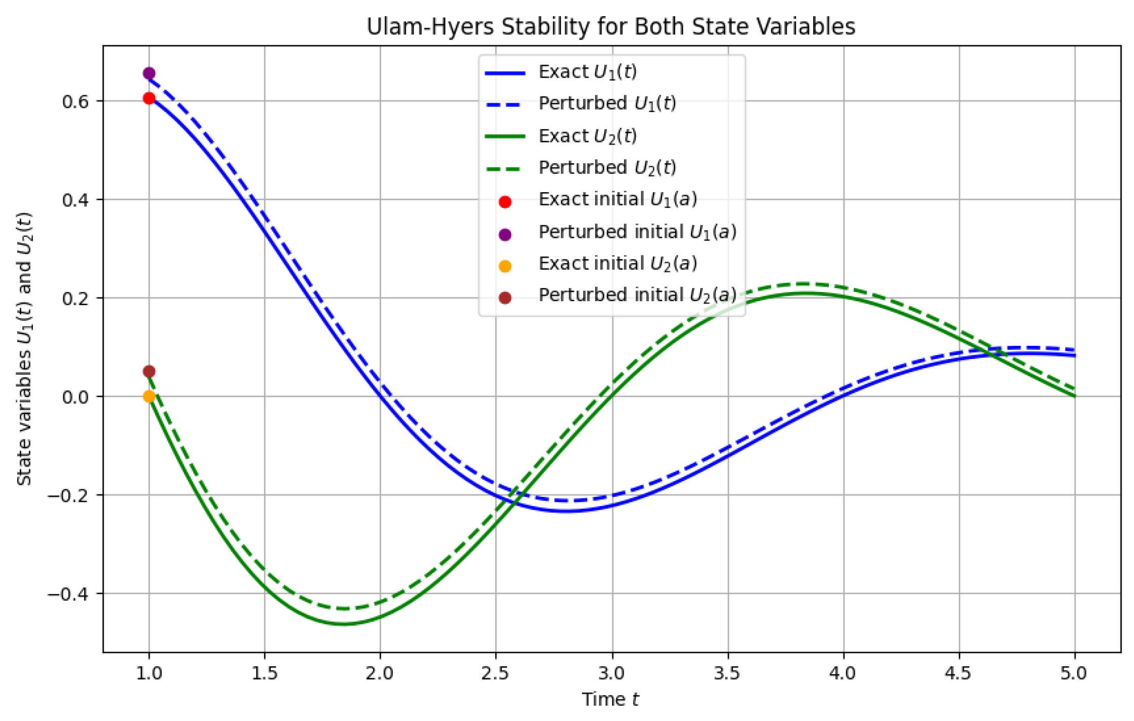
4. Stability Analysis
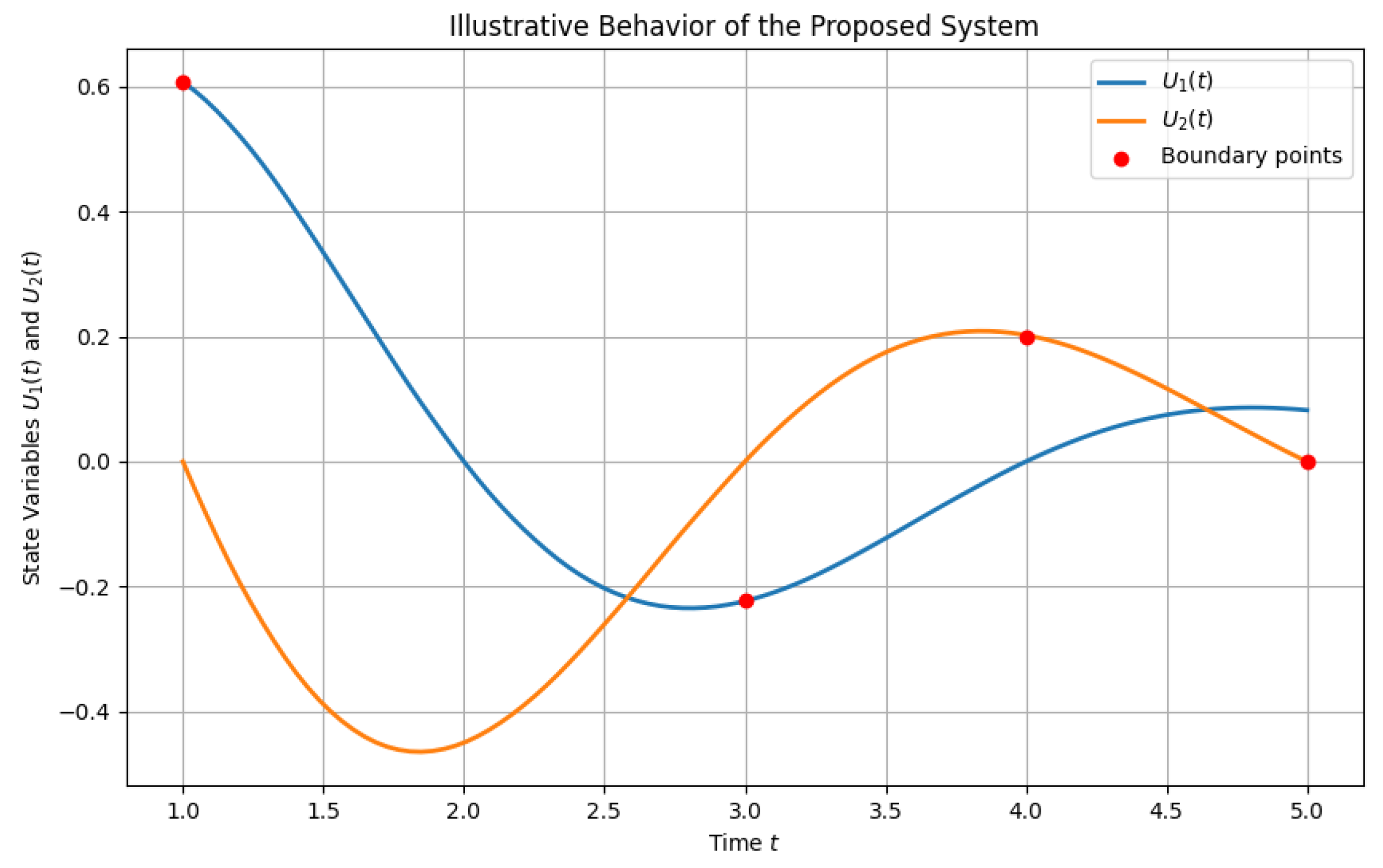
This section is devoted to the Ulam–Hyers stability for the problem at hand. We begin this section with some fundamental definitions [15].
Definition 3
([15]). For ϵ = ( ϵ 1 , ϵ 2 ) > 0 , consider the system of inequalities
| D a + r 1 H U 1 ( t ) ψ 1 ( t , U 1 ( t ) , U 2 ( t ) ) F 1 ( t , U 1 ( t ) , U 2 ( t ) ) | < ϵ 1 ; t [ a , T ] , r 1 ( 1 , 2 ] , | D a + r 2 H U 2 ( t ) ψ 2 ( t , U 1 ( t ) , U 2 ( t ) ) F 2 ( t , U 1 ( t ) , U 2 ( t ) ) | < ϵ 2 ; t [ a , T ] , r 2 ( 1 , 2 ] .
The system (2) is said to be Ulam–Hyers stable if there exists a constant c = ( c F 1 , c F 2 ) > 0 such that, for any solution ( U 1 ( t ) , U 2 ( t ) ) U 1 × U 2 of (15), there exists a unique solution ( U 1 , U 2 ) U 1 × U 2 to the system (2) satisfying the following condition:
| | ( U 1 , U 2 ) ( U ^ 1 , U ^ 2 ) | | c ϵ , t [ a , T ] .
Definition 4
([15]). If there exists a function Ψ = ( Ψ 1 , Ψ 2 ) C ( R , R ) such that Ψ ( 0 ) = 0 and Ψ 1 ( 0 ) = Ψ 2 ( 0 ) = 0 , and for every solution ( U ^ 1 , U ^ 2 ) U 1 × U 2 of (15) there exists a unique solution ( U 1 , U 2 ) U 1 × U 2 of the system (2) satisfying
( U 1 , U 2 ) ( U ^ 1 , U ^ 2 ) Ψ ( ϵ ) , t [ a , T ] ,
then the system (2) is said to be generalized Ulam–Hyers stable.
Definition 5
([16]). The system (2) is defined to be Ulam–Hyers–Rassias stable with respect to δ = ( δ 1 , δ 2 ) , where δ i C ( [ a , T ] , R ) , i = 1 , 2 , if there exist constants C = ( c F 1 , δ 1 , c F 2 , δ 2 ) > 0 such that for any ϵ = ( ϵ 1 , ϵ 2 ) > 0 and any solution ( U 1 , U 2 ) U 1 × U 2 of the system
| D a + r 1 H U 1 ( t ) ψ 1 ( t , U 1 ( t ) , U 2 ( t ) ) F 1 ( t , U 1 ( t ) , U 2 ( t ) ) | ϵ 1 δ 1 ( t ) , t [ a , T ] , | D a + r 2 H U 2 ( t ) ψ 2 ( t , U 1 ( t ) , U 2 ( t ) ) F 2 ( t , U 1 ( t ) , U 2 ( t ) ) | ϵ 2 δ 2 ( t ) , t [ a , T ] ,
there exists a unique solution ( U 1 , U 2 ) U 1 × U 2 of the system (2) satisfying the following condition:
| | ( U 1 , U 2 ) ( U ^ 1 , U ^ 2 ) | | c ϵ δ ( t ) , t [ a , T ] .
Remark 1.
(1) 
( U 1 , U 2 ) U 1 × U 2 is a solution of the system of inequalities (15) if and only if there exists functions h 1 , h 2 C ( [ a , T ] , R ) such that | h 1 ( t ) | ϵ 1 and | h 2 ( t ) | ϵ 2 , t [ a , T ] and
D a + r 1 H U 1 ( t ) ψ 1 ( t , U 1 ( t ) , U 2 ( t ) ) = F 1 ( t , U 1 ( t ) , U 2 ( t ) ) + h 1 ( t ) , t [ a , T ] , D a + r 2 H U 2 ( t ) ψ 2 ( t , U 1 ( t ) , U 2 ( t ) ) = F 2 ( t , U 1 ( t ) , U 2 ( t ) ) + h 2 ( t ) , t [ a , T ] .
(2) 
( U 1 , U 2 ) U 1 × U 2 is a solution of the system of inequalities (16) if and only if there exists functions h 1 , h 2 C ( [ a , T ] , R ) such that | h 1 ( t ) | ϵ 1 δ 1 ( t ) and | h 2 ( t ) | ϵ 2 δ 2 ( t ) , t [ a , T ] and
D a + r 1 H U 1 ( t ) ψ 1 ( t , U 1 ( t ) , U 2 ( t ) ) = F 1 ( t , U 1 ( t ) , U 2 ( t ) ) + h 1 ( t ) , t [ a , T ] , D a + r 2 H U 2 ( t ) ψ 2 ( t , U 1 ( t ) , U 2 ( t ) ) = F 2 ( t , U 1 ( t ) , U 2 ( t ) ) + h 2 ( t ) , t [ a , T ] .
Theorem 3.
Suppose that Assumption ( A 1 ) holds and Condition (14) is satisfied. Then, the system (2) is Ulam–Hyers stable. Furthermore, the system (2) is also generalized to be Ulam–Hyers stable in U 1 × U 2 .
Proof. 
Let ( U ^ 1 , U ^ 2 ) denote the unique solution of the system (2), and let ( U 1 , U 2 ) be a solution of the system of inequalities (15). By Remark (1), there exist functions h 1 , h 2 C ( [ a , T ] , R ) such that
D a + r 1 H U 1 ( t ) ψ 1 ( t , U 1 ( t ) , U 2 ( t ) ) = F 1 ( t , U 1 ( t ) , U 2 ( t ) ) + h 1 ( t ) , t [ a , T ] , D a + r 2 H U 2 ( t ) ψ 2 ( t , U 1 ( t ) , U 2 ( t ) ) = F 2 ( t , U 1 ( t ) , U 2 ( t ) ) + h 2 ( t ) , t [ a , T ] , U 1 ( t ) ψ 1 ( t , U 1 ( t ) , U 2 ( t ) ) t = a = 0 , A 1 D a + p 1 H U 1 ( t ) ψ 1 ( t , U 1 ( t ) , U 2 ( t ) ) t = T + A 2 D a + p 2 H U 1 ( t ) ψ 1 ( t , U 1 ( t ) , U 2 ( t ) ) t = T = A 3 a η 1 U 1 ( s ) d s + A 4 , U 2 ( t ) ψ 2 ( t , U 1 ( t ) , U 2 ( t ) ) t = a = 0 , B 1 D a + q 1 H U 2 ( t ) ψ 2 ( t , U 1 ( t ) , U 2 ( t ) ) t = T + B 2 D a + q 2 H U 2 ( t ) ψ 2 ( t , U 1 ( t ) , U 2 ( t ) ) t = T = B 3 a η 2 U 1 ( s ) d s + B 4
By Lemma 1, the solutions can be written explicitly as
U 1 ( t ) = ψ 1 ( t , U 1 ( t ) , U 2 ( t ) ) × ( Φ 1 ( t ) + 1 Γ ( r 1 ) a t I n t s r 1 1 F 1 ( s , U 1 ( s ) , U 2 ( s ) ) s + h 1 ( s ) d s + Φ 2 ( t ) Γ ( r 1 p 1 ) a T I n T s r 1 p 1 1 F 1 ( s , U 1 ( s ) , U 2 ( s ) ) s + h 1 ( s ) d s + Φ 3 ( t ) Γ ( r 1 p 2 ) a T I n T s r 1 p 2 1 F 1 ( s , U 1 ( s ) , U 2 ( s ) ) s + h 1 ( s ) d s + Φ 4 ( t ) Γ ( r 1 ) a η 1 a s I n s m r 1 1 F 1 ( m , U 1 ( m ) , U 2 ( m ) ) m + h 1 ( m ) d m d s ) ,
and
U 2 ( t ) = ψ 2 ( t , U 1 ( t ) , U 2 ( t ) ) × ( Θ 1 ( t ) + 1 Γ ( r 2 ) a t I n t s r 2 1 F 2 ( s , U 1 ( s ) , U 2 ( s ) ) s + h 2 ( s ) d s + Θ 2 ( t ) Γ ( r 2 q 1 ) a T I n T s r 2 q 1 1 F 2 ( s , U 1 ( s ) , U 2 ( s ) ) s + h 2 ( s ) d s + Θ 3 ( t ) Γ ( r 2 q 2 ) a T I n T s r 2 q 2 1 F 2 ( s , U 1 ( s ) , U 2 ( s ) ) s + h 2 ( s ) d s + Θ 4 ( t ) Γ ( r 2 ) a η 2 a s I n s m r 2 1 F 2 ( m , U 1 ( m ) , U 2 ( m ) ) m + h 2 ( m ) d m d s ) .
In view of | h 1 | < ϵ 1 , | h 2 | < ϵ 2 , and (11) and (12), we have
| U 1 ( t ) ψ 1 ( t , U 1 ( t ) , U 2 ( t ) ) × ( Φ 1 ( t ) + 1 Γ ( r 1 ) a t I n t s r 1 1 F 1 ( s , U 1 ( s ) , U 2 ( s ) ) s d s + Φ 2 ( t ) Γ ( r 1 p 1 ) a T I n T s r 1 p 1 1 F 1 ( s , U 1 ( s ) , U 2 ( s ) ) s d s + Φ 3 ( t ) Γ ( r 1 p 2 ) a T I n T s r 1 p 2 1 F 1 ( s , U 1 ( s ) , U 2 ( s ) ) s d s + Φ 4 ( t ) Γ ( r 1 ) a η 1 a s I n s m r 1 1 F 1 ( m , U 1 ( m ) , U 2 ( m ) ) m d m d s ) | Υ 1 ϵ 1 ,
and
| U 2 ψ 2 ( t , U 1 ( t ) , U 2 ( t ) ) × ( Θ 1 ( t ) + 1 Γ ( r 2 ) a t I n t s r 2 1 F 2 ( s , U 1 ( s ) , U 2 ( s ) ) s d s + Θ 2 ( t ) Γ ( r 2 q 1 ) a T I n T s r 2 q 1 1 F 2 ( s , U 1 ( s ) , U 2 ( s ) ) s d s + Θ 3 ( t ) Γ ( r 2 q 2 ) a T I n T s r 2 q 2 1 F 2 ( s , U 1 ( s ) , U 2 ( s ) ) s d s + Θ 4 ( t ) Γ ( r 2 ) a η 2 a s I n s m r 2 1 F 2 ( m , U 1 ( m ) , U 2 ( m ) ) m d m d s ) | Υ 2 ϵ 2 .
It follows by Assumption ( A 2 ) that
| U 1 ( t ) U ^ 1 ( t ) | Υ 1 ϵ 1 + A ψ 1 × ( Φ 1 ( t ) + 1 Γ ( r 1 ) a t I n t s r 1 1 | F 1 ( s , U 1 ( s ) , U 2 ( s ) ) F 1 ( s , U ^ 1 ( s ) , U ^ 2 ( s ) ) | d s s + Φ 2 ( t ) Γ ( r 1 p 1 ) a T I n T s r 1 p 1 1 | F 1 ( s , U 1 ( s ) , U 2 ( s ) ) F 1 ( s , U ^ 1 ( s ) , U ^ 2 ( s ) ) | d s s + Φ 3 ( t ) Γ ( r 1 p 2 ) a T I n T s r 1 p 2 1 | F 1 ( s , U 1 ( s ) , U 2 ( s ) ) F 1 ( s , U ^ 1 ( s ) , U ^ 2 ( s ) ) | d s s + Φ 4 ( t ) Γ ( r 1 ) a η 1 a s I n s m r 1 1 | F 1 ( m , U 1 ( m ) , U 2 ( m ) ) F 1 ( m , U ^ 1 ( m ) , U ^ 2 ( m ) ) | d m m d s ) | ( Υ 1 ϵ 1 ) + A ψ 1 Υ 1 μ 1 | | U 1 U ^ 1 | | + μ 2 | | U 2 U ^ 2 | | ,
which implies that
| | U 1 U ^ 2 | | ( Υ 1 ϵ 1 ) + A ψ 1 Υ 1 μ 1 | | U 1 U ^ 1 | | + μ 2 | | U 2 U ^ 2 | | ,
Similarly,
| | U 2 U ^ 2 | | ( Υ 2 ϵ 2 ) + A ψ 2 Υ 2 λ 1 | | U 1 U ^ 1 | | + λ 2 | | U 2 U ^ 2 | | .
Combining these two inequalities into a system, we apply condition (14), which ensures that
| | ( U 1 , U 2 ) ( U ^ 1 , U ^ 2 ) | | | | U 1 U ^ 1 | | + | | U 2 U ^ 2 | | Υ 1 ϵ 1 + Υ 1 ϵ 2 + ( μ i Υ 1 A ψ 1 + λ i Υ 2 A ψ 2 ) × | | U 1 U ^ 1 | | + | | U 2 U ^ 2 | | Υ 1 ϵ 1 + Υ 1 ϵ 2 1 A ψ 1 ( μ 1 + μ 2 ) Υ 1 + A ψ 2 ( λ 1 + λ 2 ) Υ 2 .
Letting c = ( c F 1 , c F 2 ) > 0 = Υ 1 1 B , Υ 2 1 B .
This guarantees that
| | ( U 1 , U 2 ) ( U ^ 1 , U ^ 2 ) | | c ϵ ,
where B = A ψ 1 ( μ 1 + μ 2 ) Υ 1 + A ψ 2 ( λ 1 + λ 2 ) Υ 2 < 1 as per Condition (14). This completes the proof that System (2) is Ulam–Hyers stable.
To show generalized Ulam–Hyers stability, we define
| | ( U 1 , U 2 ) ( U ^ 1 , U ^ 2 ) | | Ψ ( ϵ ) ,
with
Ψ ( ϵ ) = c ϵ ,
which satisfies
Ψ ( 0 ) = 0 .
This confirms generalized Ulam–Hyers stabilty. □

5. Examples

Example 1.
In this part, we present an applied example to support the theoretical results we reached in the previous part. Consider the following system:
D a + r 1 H U 1 ( t ) ψ 1 ( t , U 1 ( t ) , U 2 ( t ) ) = F 1 ( t , U 1 ( t ) , U 2 ( t ) ) ; t [ a , T ] , r 1 ( 1 , 2 ] , D a + r 2 H U 2 ( t ) ψ 2 ( t , U 1 ( t ) , U 2 ( t ) ) = F 2 ( t , U 1 ( t ) , U 2 ( t ) ) ; t [ a , T ] , r 2 ( 1 , 2 ] , U 1 ( t ) ψ 1 ( t , U 1 ( t ) , U 2 ( t ) ) t = a = 0 , A 1 D a + p 1 H U 1 ( t ) ψ 1 ( t , U 1 ( t ) , U 2 ( t ) ) t = T + A 2 D a + p 2 H U 1 ( t ) ψ 1 ( t , U 1 ( t ) , U 2 ( t ) ) t = T = A 3 a η 1 U 1 ( s ) d s + A 4 , U 2 ( t ) ψ 2 ( t , U 1 ( t ) , U 2 ( t ) ) t = a = 0 , B 1 D a + q 1 H U 2 ( t ) ψ 2 ( t , U 1 ( t ) , U 2 ( t ) ) t = T + B 2 D a + q 2 H U 2 ( t ) ψ 2 ( t , U 1 ( t ) , U 2 ( t ) ) t = T = B 3 a η 2 U 1 ( s ) d s + B 4 .
Here,
r 1 = 4 3 , r 2 = 5 4 , T = 2 , ψ 1 ( t , U 1 ( t ) , U 2 ( t ) ) ) = 5 6 sin U 1 ( t ) + 7 6 , ψ 2 ( t , U 1 ( t ) , U 2 ( t ) ) ) = 1 6 | cos U 2 ( t ) | , 3 4 = A 1 = 2 3 = B 1 , 4 5 = A 2 = 3 7 = B 2 , 3 5 = A 3 = 2 5 = B 3 , 4 7 = A 4 = 4 9 = B 4 , F 1 ( t , U 1 ( t ) , U 2 ( t ) ) ) = 7 e 5 t + 1 9 t 3 + 24 | U 2 | 1 + | U 2 | + 1 45 tan 1 U 1 , F 2 ( t , U 1 ( t ) , U 2 ( t ) ) ) = 2 e 3 t t + 1 17 tan 1 U 1 + tan 1 U 2 .
Observe that
| F 1 ( t , U 1 ( t ) , U 2 ( t ) ) ) F 1 ( t , U 2 , U 2 ) | 1 45 | U 2 U 1 | + 1 45 | U 2 U 1 | , | F 2 ( t , U 1 ( t ) , U 2 ( t ) ) ) F 2 ( t , U 2 , U 2 ) | 1 17 | U 2 U 1 | + 1 17 | U 2 U 1 | .
Then, calculate
A ψ 1 ( μ 1 + μ 2 ) Υ 1 + A ψ 2 ( λ 1 + λ 2 ) Υ 2 2 × ( 1.02738 ) × 1 45 + 1 6 × ( 1.50125 ) × 1 17 = 0.0603795 < 1 .
Thus, the boundary value problem (18) satisfies all the conditions of Theorem 2; accordingly, we conclude that the BVP has a unique solution on [ 1 , T ] .
Example 2.
Consider the following coupled hybrid fractional system:
D a + 1.5 H U 1 ( t ) ψ 1 ( t , U 1 ( t ) , U 2 ( t ) ) = F 1 ( t , U 1 ( t ) , U 2 ( t ) ) ; t [ 1 , 5 ] , D a + 1.8 H U 2 ( t ) ψ 2 ( t , U 1 ( t ) , U 2 ( t ) ) = F 2 ( t , U 1 ( t ) , U 2 ( t ) ) ; t [ 1 , 5 ] ,
on t [ 1 , 5 ] , where
ψ 1 ( t , U 1 , U 2 ) = 1 + U 1 2 + U 2 2 , ψ 2 ( t , U 1 , U 2 ) = 1 + | U 1 | + | U 2 | , a = 1 , T = 5 , r 1 = 1.5 , r 2 = 1.8 , A 1 = 0.2 , A 2 = 0.25 , A 3 = 0.1 , A 4 = 0.15 , B 1 = 0.3 , B 2 = 0.35 , B 3 = 0.05 , B 4 = 0.1 .
F 1 ( t , U 1 , U 2 ) = t sin t + U 1 + cos U 2 , F 2 ( t , U 1 , U 2 ) = t 2 + U 1 U 2
The boundary conditions are given by
U 1 ( t ) ψ 1 ( t , U 1 ( t ) , U 2 ( t ) ) t = 1 = 0 , 0.2 D 1 + 0.5 H U 1 ( t ) ψ 1 ( t , U 1 ( t ) , U 2 ( t ) ) t = T + 0.25 D 1 + 0.5 H U 1 ( t ) ψ 1 ( t , U 1 ( t ) , U 2 ( t ) ) t = T = 0.1 1 3 U 1 ( s ) d s + 0.15 , U 2 ( t ) ψ 2 ( t , U 1 ( t ) , U 2 ( t ) ) t = 1 = 0 , 0.3 D 1 + 0.8 H U 2 ( t ) ψ 2 ( t , U 1 ( t ) , U 2 ( t ) ) t = T + 0.35 D 1 + 0.8 H U 2 ( t ) ψ 2 ( t , U 1 ( t ) , U 2 ( t ) ) t = T = 0.05 1 4 U 1 ( s ) d s + 0.1 ,
For this system, the constants associated with the nonlinear terms are as follows:
A ψ 1 = 2 , A ψ 2 = 1.5 , Υ 1 = 1 , Υ 2 = 1
K 1 = 0.1 , K 2 = 0.1 , L 1 = 0.1 , L 2 = 0.1
The condition required by Theorem 2 holds:
A ψ 1 K 1 Υ 1 + A ψ 2 L 1 Υ 2 = 0.35 < 1
A ψ 1 K 2 Υ 1 + A ψ 2 L 2 Υ 2 = 0.35 < 1
Thus, by Theorem 2, the system admits a unique solution in C ( [ 1 , 5 ] , R 2 ) .
The following two graphs complement the theoretical analysis by providing a visual demonstration of the system’s behavior and stability. The first graph shows the general time evolution of U 1 and U 2 , while the second graph compares exact and perturbed solutions to verify the system’s Ulam–Hyers stability.
The graph in Figure 1 illustrates the behavior of the system’s state variables U 1 ( t ) and U 2 ( t ) over time. Both solutions exhibit a damped oscillatory behavior, which reflects the fractional-order memory effects incorporated through the Hadamard fractional derivatives. The presence of exponential decay coupled with oscillatory motion is a typical characteristic of fractional systems, where memory and hereditary effects influence the evolution of each state variable.
The marked boundary points t = a and t = T correspond to the non-local conditions imposed in the system. These conditions introduce a coupling between the two components U 1 and U 2 , reinforcing the hybrid nature of the system.
This visual representation confirms that the analytical framework developed in this paper captures realistic and physically meaningful behaviors for hybrid fractional systems. It also illustrates how a fractional order (such as r 1 and r 2 ) controls the rate of decay and the frequency of oscillation, offering flexibility in modeling real-world processes where long-term memory and non-local interactions play a significant role.
Figure 2 illustrates the Ulam–Hyers stability of the proposed system by comparing the exact solutions U 1 ( t ) and U 2 ( t ) to perturbed solutions initialized with a small deviation at t = a . Both components maintain close trajectories, demonstrating that the system’s solutions are robust against small perturbations in initial conditions. This confirms the theoretical Ulam–Hyers stability established earlier.

6. Conclusions

In this paper, we analyzed a coupled system of hybrid fractional differential equations involving Hadamard fractional derivatives under non-local boundary conditions. We successfully established conditions for existence and uniqueness using two complementary approaches: Banach’s fixed point theorem and the Leray–Schauder alternative. Furthermore, we demonstrated that the system satisfies Ulam–Hyers stability as well as generalized Ulam–Hyers stability, meaning that small perturbations in initial data only lead to controlled deviations in the solution. This confirms both the well-posedness and robustness of the proposed system.
Future directions include applying this framework to multi-component hybrid systems, extending the analysis to variable-order Hadamard operators, and considering more flexible boundary settings, such as fractional feedback controls. Additionally, developing efficient numerical algorithms tailored to Hadamard-type hybrid fractional systems would be an important step to support practical simulations and real-world applications.

Author Contributions

Conceptualization, M.A.; Methodology, M.A. and M.M.; Formal analysis, M.A.A. and M.A.; Investigation, M.A.A. and J.A.; Writing—original draft, M.M. and M.A.; Writing—review and editing, M.M. and M.A.; Supervision, M.A.A. and M.A. All authors have read and agreed to the published version of the manuscript.

Funding

This work was supported by the Deanship of Scientific Research, Vice Presidency for Graduate Studies and Scientific Research, King Faisal University, Saudi Arabia [Grant No. KFU250991]. This study was supported via funding from Prince Sattam bin Abdulaziz University, project number (PSAU/2025/R/1446). M. Manigandan would like to thank SRM TRP Engineering College, India, for their financial support, vide number SRM/TRP/RI/005.

Data Availability Statement

No data were used for the research described in the article.

Conflicts of Interest

The authors declare no conflicts of interest.

References

  1. Podlubny, I. Fractional Differential Equations: An Introduction to Fractional Derivatives, Fractional Differential Equations, to Methods of Their Solution and Some of Their Applications; Elsevier: Amsterdam, The Netherlands, 1998. [Google Scholar]
  2. Milici, C.; Drăgănescu, G.; Machado, J.T. Introduction to Fractional Differential Equations; Springer: Berlin/Heidelberg, Germany, 2018; Volume 25. [Google Scholar]
  3. Demirci, E.; Karakoç, F.; Kütahyalıoglu, A. Mittag-Leffler stability of neural networks with Caputo–Hadamard fractional derivative. Math. Methods Appl. Sci. 2024, 47, 10091–10100. [Google Scholar] [CrossRef]
  4. Liu, W.; Liu, L. Properties of Hadamard fractional integral and its application. Fractal Fract. 2022, 6, 670. [Google Scholar] [CrossRef]
  5. Kilbas, A.A.; Srivastava, H.M.; Trujillo, J.J. Theory and Applications of Fractional Differential Equations; Elsevier: Amsterdam, The Netherlands, 2006; pp. 82–89. [Google Scholar]
  6. Debnath, P.; Srivastava, H.M.; Kumam, P.; Hazarika, B. Fixed Point Theory and Fractional Calculus: Recent Advances and Applications; Springer: Berlin/Heidelberg, Germany, 2022. [Google Scholar]
  7. Wardowski, D. Fixed points of a new type of contractive mappings in complete metric spaces. Fixed Point Theory Appl. 2012, 2012, 94. [Google Scholar] [CrossRef]
  8. Zafar, R.; Rehman, M.U.; Shams, M. On Caputo modification of Hadamard-type fractional derivative and fractional Taylor series. Adv. Differ. Equ. 2020, 2020, 219. [Google Scholar] [CrossRef]
  9. Balachandran, K.; Matar, M.; Annapoorani, N.; Prabu, D. Hadamard functional fractional integrals and derivatives and fractional differential equations. Filomat 2024, 38, 779–792. [Google Scholar] [CrossRef]
  10. Murugesan, M.; Muthaiah, S.; Alzabut, J.; Nandha Gopal, T. Existence and HU stability of a tripled system of sequential fractional differential equations with multipoint boundary conditions. Bound. Value Probl. 2023, 2023, 56. [Google Scholar] [CrossRef]
  11. Subramanian, M.; Manigandan, M.; Zada, A.; Gopal, T.N. Existence and Hyers–Ulam stability of solutions for nonlinear three fractional sequential differential equations with nonlocal boundary conditions. Int. J. Nonlinear Sci. Numer. Simul. 2023, 24, 3071–3099. [Google Scholar] [CrossRef]
  12. Wang, J.; Li, X. A uniform method to Ulam–Hyers stability for some linear fractional equations. Mediterr. J. Math. 2016, 13, 625–635. [Google Scholar] [CrossRef]
  13. Zada, A.; Ali, W.; Farina, S. Hyers–Ulam stability of nonlinear differential equations with fractional integrable impulses. Math. Methods Appl. Sci. 2017, 40, 5502–5514. [Google Scholar] [CrossRef]
  14. Jakhar, J.; Sharma, S.; Jakhar, J.; Yousif, M.A.; Mohammed, P.O.; Chorfi, N.; Vivas-Cortez, M. Hyers–Ulam–Rassias Stability of Functional Equations with Integrals in B-Metric Frameworks. Symmetry 2025, 17, 168. [Google Scholar] [CrossRef]
  15. Rus, I.A. Ulam stabilities of ordinary differential equations in a Banach space. Carpathian J. Math. 2010, 26, 103–107. [Google Scholar]
  16. Khan, S.; Shah, K.; Debbouche, A.; Zeb, S.; Antonov, V. Solvability and Ulam-Hyers stability analysis for nonlinear piecewise fractional cancer dynamic systems. Phys. Scr. 2024, 99, 025225. [Google Scholar] [CrossRef]
  17. Subramanian, M.; Manigandan, M.; Gopal, T.N. Fractional differential equations involving Hadamard fractional derivatives with nonlocal multi-point boundary conditions. Discontin. Nonlinearity Complex. 2020, 9, 421–431. [Google Scholar] [CrossRef]
  18. Zhao, D.; Luo, M. Representations of acting processes and memory effects: General fractional derivative and its application to theory of heat conduction with finite wave speeds. Appl. Math. Comput. 2019, 346, 531–544. [Google Scholar] [CrossRef]
  19. Vabishchevich, P.N. Numerical solution of the heat conduction problem with memory. Comput. Math. Appl. 2022, 118, 230–236. [Google Scholar] [CrossRef]
  20. Al Elaiw, A.; Awadalla, M.; Manigandan, M.; Abuasbeh, K. A novel implementation of Mönch’s fixed point theorem to a system of nonlinear Hadamard fractional differential equations. Fractal Fract. 2022, 6, 586. [Google Scholar] [CrossRef]
  21. Abuasbeh, K.; Awadalla, M.; Jneid, M. Nonlinear Hadamard fractional boundary value problems with different orders. Rocky Mountain J. Math. 2021, 51, 17–29. [Google Scholar] [CrossRef]
  22. Mahmudov, N.I.; Awadalla, M.; Abuassba, K. Hadamard and caputo-hadamard FDE’s with three point integral boundary conditions. Nonlinear Anal. Differ. Equ. 2017, 5, 271–282. [Google Scholar] [CrossRef]
  23. Agrawal, O. Fractional variational calculus in terms of Riesz fractional derivatives. J. Phys. Math. Theor. 2007, 40, 6287. [Google Scholar] [CrossRef]
  24. Liu, W.; Liu, L. Existence of solutions for the initial value problem with hadamard fractional derivatives in locally convex spaces. Fractal Fract. 2024, 8, 191. [Google Scholar] [CrossRef]
  25. Almeida, R.; Torres, D.F. Necessary and sufficient conditions for the fractional calculus of variations with Caputo derivatives. Commun. Nonlinear Sci. Numer. Simul. 2011, 16, 1490–1500. [Google Scholar] [CrossRef]
  26. Boutiara, A.; Guerbati, K.; Benbachir, M. Caputo Hadamard fractional differential equation with three-point boundary conditions in Banach spaces. Aims Math. 2019, 5, 259–272. [Google Scholar]
Figure 1. Illustrative behavior of the state variables U 1 ( t ) and U 2 ( t ) for the proposed hybrid fractional system.
Mathematics 13 00941 g001
Figure 2. Ulam–Hyers stability demonstration for both state variables U 1 ( t ) and U 2 ( t ) .
Mathematics 13 00941 g002
Disclaimer/Publisher’s Note: The statements, opinions and data contained in all publications are solely those of the individual author(s) and contributor(s) and not of MDPI and/or the editor(s). MDPI and/or the editor(s) disclaim responsibility for any injury to people or property resulting from any ideas, methods, instructions or products referred to in the content.

