Abstract
Solving satisfiability problems is central to many areas of computer science, including artificial intelligence and optimization. Efficiently solving satisfiability problems requires exploring vast search spaces, where search space partitioning plays a key role in improving solving efficiency. This paper defines search spaces and their partitioning, focusing on the relationship between partitioning strategies and satisfiability problem solving. By introducing an abstraction method for partitioning the search space—distinct from traditional assignment-based approaches—the paper proposes sequential, parallel, and hybrid solving algorithms. Experimental results show that the hybrid approach, combining abstraction and assignment, significantly accelerates solving in most cases. Furthermore, a unified method for search space partitioning is presented, defining independent and complete partitions. This method offers a new direction for enhancing the efficiency of SAT problem solving and provides a foundation for future research in the field.
MSC:
68T20
1. Introduction
The SAT (satisfiability) problem involves determining whether a given Boolean formula has a satisfiable assignment. As one of the classical problems in computer science and among the most notable NP-complete problems in computational complexity theory [1], SAT has been extensively studied and discussed for nearly a century. Due to its critical role in formal verification [2,3], artificial intelligence [4], and combinatorial optimization [5], efficiently solving SAT problems remains a key focus of research.
From the most straightforward perspective, solving a SAT problem entails traversing the search space. As the problem size increases, the search space expands exponentially, resulting in exponentially growing solving times, which makes direct solving infeasible for large-scale problems. To improve solving efficiency, heuristic strategies are widely employed in SAT solving [6]. The core algorithm of modern SAT solvers, conflict-driven clause learning (CDCL), significantly accelerates solving by utilizing heuristics such as clause learning, conflict-driven backjumping, and decision heuristics, building upon the foundational DPLL algorithm [7].
When employing DPLL or CDCL algorithms, the problem is solved sequentially [8], iteratively verifying potential assignments via backjumping. To further enhance solving efficiency, leveraging computational resources through parallel computation becomes another key approach. Inspired by parallelism, SAT parallel solvers have seen significant development. The two primary categories of mainstream parallel SAT solving algorithms are as follows [9,10]:
- (1)
- Divide-and-conquer algorithms, which partition the search space and compute different portions in parallel.
- (2)
- Portfolio algorithms, which employ multiple solvers with diverse restart, decision, and learning heuristics applied to parallel instances, competing to find the fastest solving path.
In both sequential and parallel solving, the essence of SAT solving lies in assigning values (1 or 0) to one or more variables and analyzing their impact on formula satisfiability through operations like constraint propagation and conflict analysis. This paper defines the search space from both topological and logical perspectives, analyzing the nature of assignments and revealing their essence as partitions of the search space.
Based on this insight, a novel search space partitioning method is proposed, differing from traditional assignment-based approaches. This method partitions the search space by merging variables, not only independently deriving sequential or parallel solving algorithms, but also being combined with assignment strategies. Experimental data indicate that, depending on the algorithm strategy, the solving time can be optimized in the majority of cases. Finally, the paper summarizes a more unified search space partitioning methodology, rigorously defining the properties of different partitions and providing a more precise analysis of various existing solving algorithms.
Organization of the Paper:
- Section 2: Reviews the most common SAT solving algorithms as well as the various solvers that implement these algorithms;
- Section 4: Explains how this new approach can be applied in solving, offering ideas for both sequential and parallel solving while discussing its interaction with the existing methods;
- Section 5: Summarizes a unified search space partitioning method, defines the properties of partitions, and analyzes the partition characteristics satisfied by the existing solving algorithms.
2. Overview of SAT Solving
2.1. Common Solving Algorithms
The most critical aspect of SAT solving is the algorithm, as the algorithm determines the foundation and underlying logic of the entire SAT solving process. Therefore, understanding the most important algorithms in SAT solving is essential.
2.1.1. Sequential Algorithms: DPLL and CDCL
The DPLL algorithm (Davis–Putnam–Logemann–Loveland Algorithm) is a classical method for solving the satisfiability problem (SAT). Proposed in 1962 by Martin Davis, Hilary Putnam, George Logemann, and Donald Loveland, it is an improvement of the earlier Davis–Putnam algorithm. Viewing the SAT solving process as traversing a decision tree, DPLL is a complete search algorithm that employs backtracking and pruning strategies [11].
Example 1.
Illustration of SAT solving process using DPLL and unit propagation.
Given the following formula,
Decision:
.
By assigning , the formula simplifies through unit propagation:
Unit Propagation: .
Unit propagation forces , due to the clause . When simplifying further,
At this stage, a conflict occurs, as cannot simultaneously satisfy both and .
Backtracking: .
Backtrack and assign . The formula now simplifies to the following:
Pure Literal Elimination: , .
Here, and are pure literals (appearing with consistent polarity). Assign and , resulting in a satisfiable formula.
Conclusion
Formula F is satisfiable with the following assignment: , , .
From Example 1 and Figure 1, it can be observed that the search tree of formula and the DPLL algorithm’s search tree demonstrate how DPLL explores the search space by assigning values to variables and backtracking when encountering unsatisfiable states.
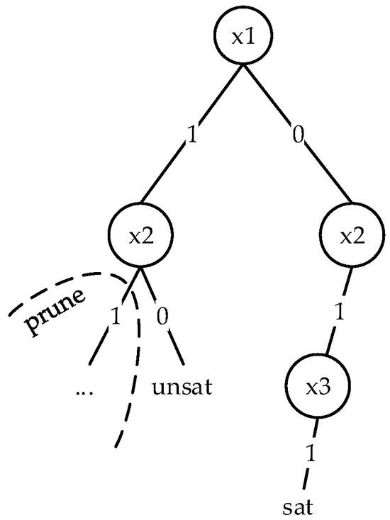
Figure 1.
Decision tree for SAT solving based on formula .
Conflict-driven clause learning (CDCL), building upon DPLL, incorporates additional strategies. The most critical of these is analyzing the cause of conflicts upon encountering an unsatisfiable state. This analysis transforms backtracking into backjumping [12,13], effectively skipping unnecessary local backtracking.
Various CDCL-based solvers achieve further optimization by improving or introducing additional pruning strategies, enhancing the overall efficiency of the solving process.
In both DPLL and CDCL, unit propagation is the most commonly used and essential technique for reducing the search space through pruning [14]. Unit propagation analyzes the clauses affected by existing assignments. If a clause contains only one unassigned literal, that literal is forced to take a value of 1 or 0 to satisfy the clause under the current assignment. This approach avoids blindly selecting variable assignments and significantly accelerates the solving process.
In summary, backtracking determines how to retreat during the search, while unit propagation largely dictates how to advance the search efficiently.
2.1.2. Parallel Algorithms: DAC and Portfolios
Currently, mainstream parallel SAT solving methods can be categorized into two types:
Portfolio-based solving: Tools like ManySAT [15], Hordesat [16], and SArTagnan [17] employ this approach. These methods simultaneously create multiple solving instances using diverse restart [18] and decision strategies. The solving process is completed as soon as the fastest instance finishes.
Divide-and-conquer-based solving: This method, which is the focus of this paper, attempts to accelerate solving by dividing the search space into smaller segments and solving them in parallel. A commonly used method for dividing the search space is guiding paths [19], which is intuitive and straightforward. It assigns variables of 0 or 1 to partition the search space. For instance, assigning and creates two parallel instances, while assigning and simultaneously creates four instances.
Figure 2a,b illustrate these two parallel solving strategies.
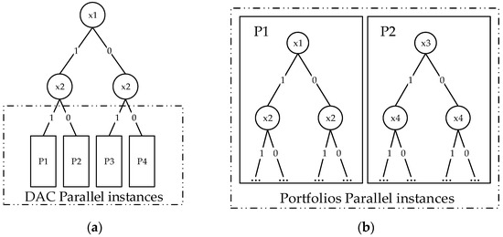
Figure 2.
Parallel solving strategies. (a) DAC parallel instances: the search space is divided using guiding paths, with each subspace solved independently in parallel. (b) Portfolio parallel instances: multiple solvers explore the full search space using different strategies, such as distinct pruning or restart methods.
For Figure 2b (Portfolio Solving), multiple search trees are created, each utilizing different pruning or restart strategies, resulting in varied search paths. Since each tree covers the entire search space, the solving status of the formula can be determined as soon as one tree finds a satisfiable assignment or confirms unsatisfiability.
In contrast, Figure 2a (DAC Solving) demonstrates a single search tree divided into multiple subtrees for parallel solving. Unlike Portfolio Solving, DAC requires all subtrees to confirm unsatisfiability to conclude that the original formula is unsatisfiable. Notably, the computation within each subtree uses sequential algorithms such as CDCL [9], making it possible to combine this method with Portfolio Solving for enhanced performance.
With the increase in computational resources, parallel computing has gradually shifted its focus to leveraging the parallel computing advantages of GPUs [20,21]. Numerous parallel computing methods utilizing GPU acceleration have been continuously proposed.
Although parallel solving may seem straightforward, its core lies in optimizing communication and coordination between instances [21]. Mechanisms such as clause sharing [22] and search path sharing [18] are particularly critical for improving the efficiency of parallel solving.
In summary, DPLL laid the theoretical foundation for SAT solving, but its efficiency is limited by its backtracking and pruning capabilities. CDCL significantly improved single-threaded solving performance through conflict analysis and clause learning, yet it still encounters bottlenecks when handling complex problems. Parallel solving, including portfolio and divide-and-conquer approaches, has greatly enhanced solving capabilities. However, communication and coordination between instances (e.g., clause sharing and path management) remain key challenges affecting parallel efficiency and require further optimization.
2.2. Implementation in Sat Solvers
Traditional SAT solvers are mostly based on the classical DPLL and CDCL algorithms, which explore the solution space step by step through variable assignments and backtracking, and accelerate the solving process using techniques such as conflict-driven clause learning (CDCL). For example, MiniSAT [23], a classic complete solver, is widely used for solving SAT problems and has demonstrated good performance in many practical scenarios. Another complete solver, Z3 [24], was initially designed as an SMT solver, but also performs very well when handling SAT problems. The advantage of complete solvers is that they guarantee finding a solution (if one exists), but their completeness often results in longer solving times when dealing with large-scale or complex SAT instances.
For large-scale or complex problems, full solving is often very difficult, which is why many incomplete solvers use local search and heuristic methods to find approximate solutions, improving solving efficiency. For example, walkSAT [25] uses a randomized local search strategy to quickly find a satisfying solution in the solution space, typically yielding a feasible solution within a short period, although it cannot guarantee finding all solutions. Another incomplete solver, CryptoMiniSat [26], combines randomization and heuristic methods in its search process to optimize solving.
As problem sizes continue to grow, traditional algorithms and solvers, while highly complete, often face computational bottlenecks in certain cases, prompting researchers to explore new solving methods. In this context, the widespread adoption of new technologies such as GPU acceleration and deep learning in SAT solving has been seen in recent years, making them popular research directions today. GPU-accelerated solvers are primarily parallel solvers that fully leverage the advantages of GPU parallel computing, greatly improving the efficiency of solving large-scale problems, especially in hardware verification and artificial intelligence. GPU-based SAT solvers, such as the PicoSAT [27] GPU version, can process massive datasets quickly. At the same time, deep learning techniques have started to be integrated with traditional SAT solving methods, bringing new advances. Solvers like DeepSAT [28] and SATNet [29] optimize search strategies using neural networks and predict variable assignments based on learning from large datasets, reducing backtracking and conflicts. The introduction of deep learning not only enhances solving speed, but also provides new ideas for the intelligence and automation of SAT solvers.
In addition to the solvers mentioned above, many novel solving methods are continuously being researched, and a brief description of these methods is provided in Table 1.

Table 1.
Overview of newest SAT solving methods.
Although different solvers employ cutting-edge technologies, most of them have not completely abandoned the traditional mechanisms of variable assignment and backtracking in their solving principles. New technologies, such as deep learning, primarily serve to assist in optimizing the search process and parameters, making solving more efficient.
3. Search Space and Partitioning
In the previous section, we briefly introduced some SAT solving algorithms, both parallel and sequential. Regardless of the approach, these algorithms ultimately assign values to variables in a step-by-step process, to either find a satisfying assignment for the formula or prove that the original formula is unsatisfiable. We can refer to this solving process as assignment-based solving. In this section, we propose a new solving approach that differs from the traditional assignment-based methods. This approach involves merging variables, which we refer to as abstraction.
To better explain the distinction between abstraction and assignment, we must introduce the concept of search space and intuitively analyze the differences and connections between the two.
3.1. Definition of Search Space
In this study, we use CNF formulas to represent SAT problems. For clarity, we define the following terminology for SAT problems:
- Let represent a CNF formula and represent a disjunction. Thus, represents a CNF formula consisting of disjunctions , where each is a clause of the formula F;
- The set of variables appearing in the formula is denoted as , and the set of variables appearing in a clause is denoted as , represented by ;
- To maintain symmetry in the search space, in this paper, we assign the value for true and for false (instead of x = 0). A set of satisfiable assignments is called a solution to the formula, denoted by , and the set of all solutions is denoted by .
For example, if and , then represents the formula . and are two sets of assignments for the formula F, and .
Definition 1.
Given formula , the search space of is defined as , denoted as .
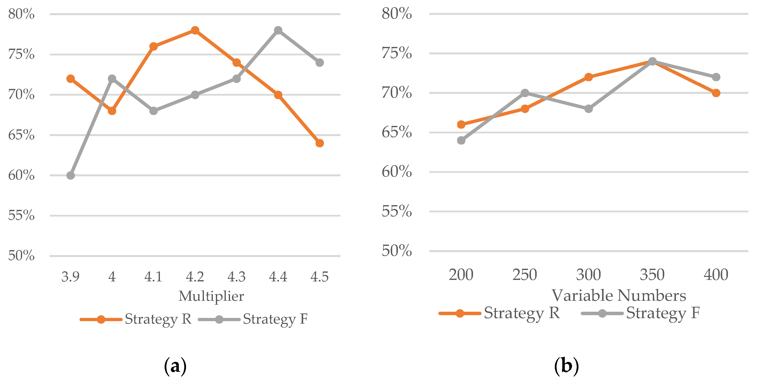
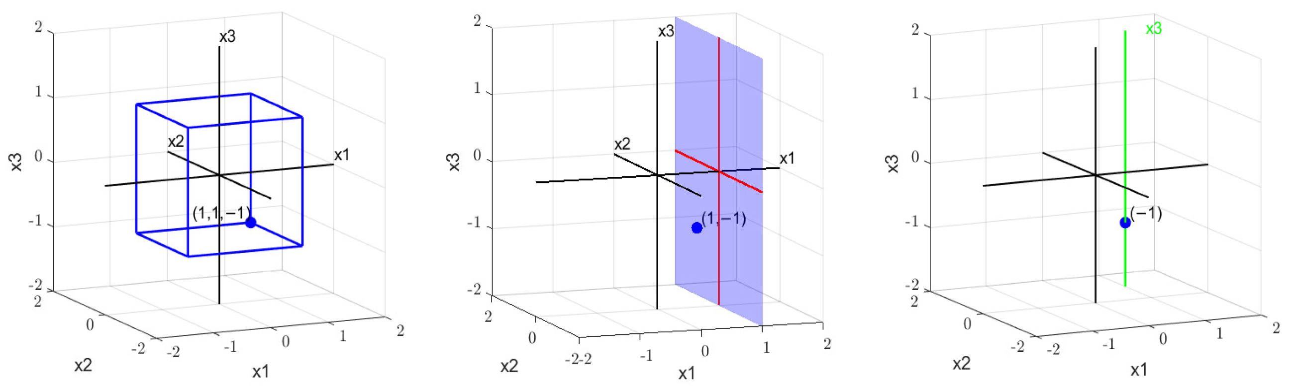
According to Definition 1, is the set of vertices of a hyperrectangle centered at the origin, with edges parallel to the coordinate axes. Suppose we have two formulas:
For formula , with , .
For formula , with , .
The solutions of these formulas in the search space are shown in Figure 3.

Figure 3.
Search space examples. (a) Search space of . (b) Search space of .
3.2. Assignment-Based Solving and Its Partitioning
3.2.1. Logical Expression of Assignment-Based Solving
As mentioned earlier, in commonly used SAT solving algorithms, variables are assigned values step by step. Assigning a value of 1 to a variable in formula can be viewed as the formula . Similarly, assigning a value of −1 corresponds to the formula [9].
Taking the first three formulas in Example 1, , as an example, the result when is shown in Table 2.
Table 2.
Results of assigning to each clause.
We can simplify the formula and obtain . Next, we observe the formula , and the results are shown in Table 3, where each clause can also be simplified.
Table 3.
Results of each clause when the formula is conjoined with .
The resulting formula is . Assigning produces the same results as . Furthermore, in order for the formula to be satisfiable, must also be 1.
In other words, logically, the assignment of values to the formula is equivalent to , and the simplification after assignment is equivalent to applying the absorption law and resolution to the formula .
At the same time, if the simplified formula obtained after assigning is satisfiable, it indicates that the original formula is also satisfiable. However, if is unsatisfiable, it does not necessarily imply that the original formula is also unsatisfiable. This can also be explained logically.
Proposition 1.
If the formula is satisfiable, then the formula is satisfiable.
Proof.
If is satisfiable, then there exists an assignment such that . is equivalent to AND . Therefore, if is satisfiable, it implies that is satisfiable. □
Proposition 2.
If the formula is unsatisfiable, then the formula is not necessarily unsatisfiable.
Proof.
If is unsatisfiable, then for all assignments , . is equivalent to OR . This means that it is possible for to be satisfiable while is unsatisfiable, if is unsatisfiable under the given assignment. Therefore, the unsatisfiability of does not necessarily imply the unsatisfiability of □
Therefore, determining the satisfiability of the original formula by checking whether the simplified formulas for and are satisfiable is equivalent to determining the satisfiability of the formula , which, after simplification, becomes .
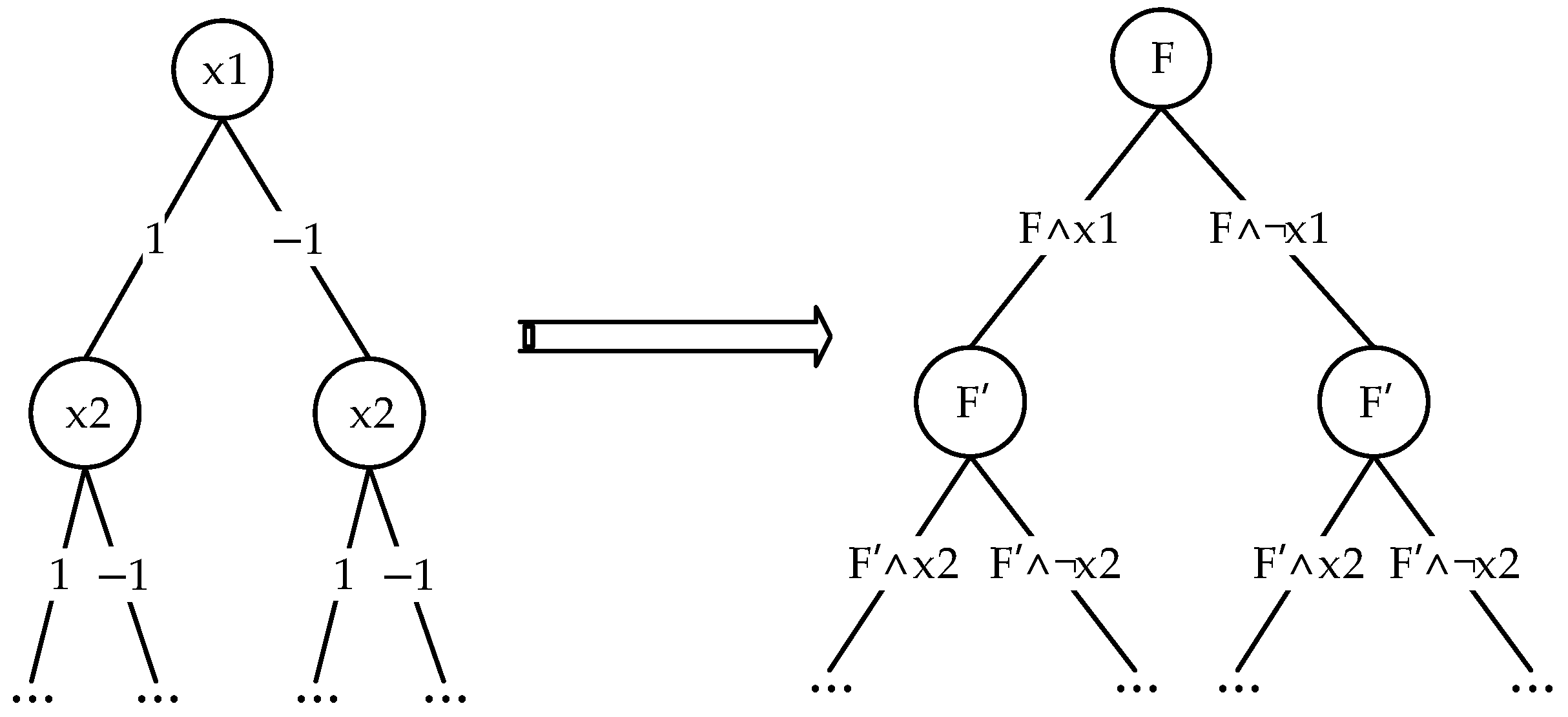
From a logical perspective, the assignment-based backtracking algorithm essentially repeats the following steps:
If is satisfiable, then must be satisfiable. To check if is satisfiable, one can further check if is satisfiable, and so on.
Similarly, if is unsatisfiable, then it is necessary to check if is satisfiable. To check if is satisfiable, one can continue checking if is satisfiable, progressing step by step.
The search tree of the assignment-based SAT solving algorithm is logically equivalent to the search tree shown in Figure 4.

Figure 4.
Search tree of the assignment-based SAT solving algorithm.
3.2.2. Partitioning of Assignment-Based Solving
As we learned in the previous section, assignment essentially adds new constraints to the formula. Next, we will explore how these constraints affect the search space.
Definition 2.
Given formulas and , if , then is called a logical partition of . The formula is referred to as a partition of the search space of , and is called the partitioned formula.
Example 2.
Solving a Formula Using Assignments.
Formula :
If we simulate the assignment process, we first try assigning and use unit propagation, which simplifies the formula to:
Next, we assign , which leaves us with the final clause:
Thus, we obtain a satisfiable assignment .
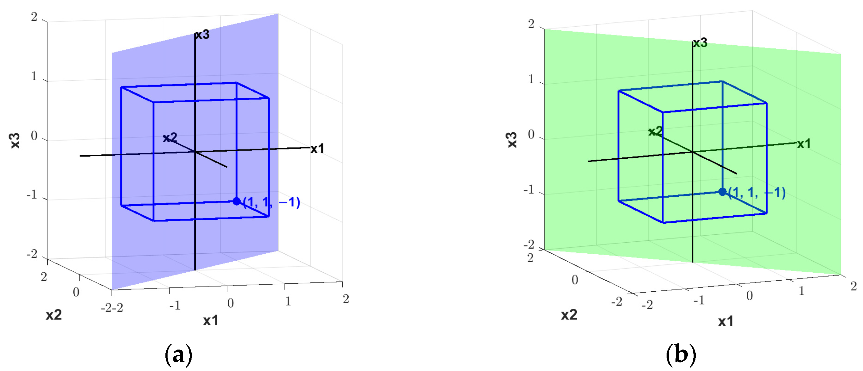
If we plot the solution and search spaces of the three formulas , , and , as shown in Figure 5, we can observe the following:
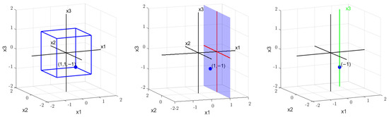
Figure 5.
Process of partitioning the search space.
Assigning corresponds to using the plane to cut the search space , resulting in the space partition .
Assigning corresponds to using the line to cut the search space , resulting in the partition .
The entire process involves progressively reducing the dimensions. Each assignment lowers the dimensionality, and when the dimension reaches one, we can check whether the formula has a solution at that point.
As shown in Figure 6, both and partition the formula . They represent the planes and , respectively. If no solution is found on the plane (the green plane), as seen in the previous search tree, backtracking is used to check for an assignment on (the blue plane). If no solution is found on either plane, it means that no solution exists within this three-dimensional search space. Similarly, this three-dimensional search space may be derived from a four-dimensional space by partitioning with . The next step would involve backtracking to the partition of .
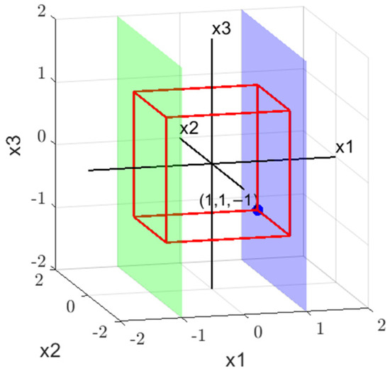
Figure 6.
Three-dimensional search space.
Therefore, the backtracking algorithm continuously partitions the search space and ultimately verifies whether a point in the search space is a solution to the formula. Parallel algorithms based on search space partitioning also stem from this backtracking process, but they calculate multiple backtracking paths simultaneously. In addition to this assignment-based search space partitioning, there are other partitioning methods. In this paper, we propose a new search space partitioning method, referred to as abstraction-based search space partitioning.
3.3. Abstraction-Based Solving and Its Partitioning
As mentioned in the previous section, assignment-based solving is essentially solving the two partitioned formulas, and . As long as one of them is satisfiable, the original formula is satisfiable. This is expressed as follows:
This conclusion holds for any formula, meaning that:
As defined in Definition 1 from the previous section, adding constraints corresponds to partitioning the search space. In other words, and are actually methods of partitioning the search space. The constraints added by the assignment, and , partition using the hyperplanes and , respectively. Each partition reduces the dimensionality by eliminating , and through continuous dimensional reduction, a solution is verified.
If we consider dimensional reduction, there are also other methods for reducing dimensions.
Observing the search space partitioning method shown in Figure 7, the search space is partitioned using the planes (a) and (b). In both planes, the dimension is preserved, while the dimensions and are merged into a new dimension. The two planes together form the original search space in its entirety.
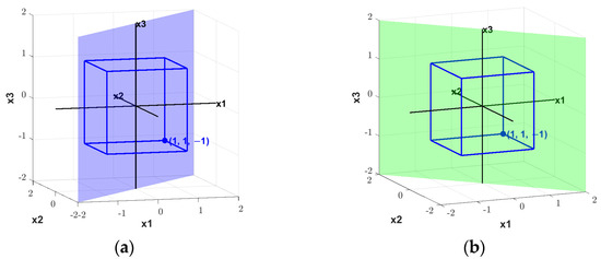
Figure 7.
Another approach to partitioning. (a) Plane , (b) plane .
We can extend this merging method to higher-dimensional search spaces by partitioning the space with the hyperplanes and , effectively merging dimensions and to achieve dimensional reduction. To do this, we need to provide a clear definition of such an operation.
In Answer Set Programming (ASP), researchers have developed a debugging method that maps multiple propositional atoms to a set , which is called Omission-based Abstraction [34]. The merging and dimensional reduction process is similar to this, but instead of omitting atoms, it merges multiple propositional variables and substitutes them with a new variable. Therefore, we can also refer to this operation as abstraction.
Definition 3.
Let be a formula with . If the mapping holds, where and , the new formula obtained is called the abstraction of formula , denoted as .
Abstraction defines the merging of dimensions and , with the new dimension denoted as . From a logical perspective, the mapping is equivalent to . In Boolean formulas, is equivalent to .
As we learned in Section 3.2.1, the simplification of formulas in assignment-based solving is based on resolution and the absorption law. Just as assignments can simplify the original formula, abstraction can also simplify a formula. As shown in Table 4, the simplification of the abstracted formula is also based on resolution.
Table 4.
The impact of abstraction on clauses.
That is, .
The clause and the constraint resolve to , which is equivalent to . Similarly, and resolve to , which is equivalent to . We have mapped both and to , thus obtaining and .
Lemma 1.
.
Now, we have the logical representation of the hyperplane . Since we define False as −1, the symmetry of the search space allows us to use the formula to represent the plane . To represent , we can generalize extended Definition 3.
In Definition 3, the mapping , i.e., , is essentially a mapping of variables. This includes both and . Similarly, if we perform such a mapping, and , we can denote it as .
Definition 3 (continued).
Let be a formula with . If the mapping holds, where and , the new formula obtained is called the abstraction of formula , denoted as .
Similarly, from a logical perspective, this abstraction corresponds to solving , which is equivalent to . As shown in Table 5, The clauses in also come from the resolution of the original formula’s clauses with or , followed by the variable mapping.
Table 5.
The impact of extended abstraction on clauses.
That is, .
Thus, we can draw similar conclusions.
Lemma 2.
.
The mapping process represented by abstraction is the merging of dimensions and , with the new dimension denoted as . This gives us a partitioning method that is different from assignment-based partitioning, namely, abstraction-based partitioning.
The abstraction-based partitioning formulas are as follows: or , which correspond to and , respectively.
4. Abstraction-Based Solving Method
In this section, we will propose the methodology for abstraction-based solving, drawing on the existing assignment-based solving methods. We will also introduce a hybrid solving method that combines abstraction and assignment.
4.1. Conventional Solving Methods
In Section 3.2.1, we used a search tree to describe the logical form of assignment-based solving. Similarly, abstraction-based solving should also be represented in this manner, as shown in Figure 8.
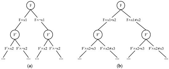
Figure 8.
Search tree of abstraction-based solving and assignment-based solving. (a) Search tree of assignment-based solving, (b) search tree of abstraction-based solving.
If the assignment-based solving algorithm is described by the following steps: Assignment → Simplification → Backtracking → Assignment → … then, similarly, the abstraction-based solving algorithm should be divided into these steps: Abstraction → Simplification → Backtracking → Abstraction → …
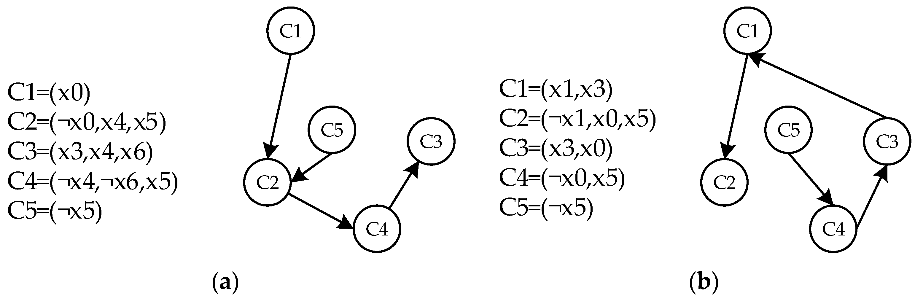
For the formula , abstraction-based solving can proceed according to the process shown in Table 6.
Table 6.
Abstraction-based solving process.
Only in the final path, where the formula simplifies to , does a solution exist, with . Then, via and , we obtain .
In assignment-based solving, each time a variable is assigned a value, its assignment is recorded. In contrast, abstraction-based solving is more like a classifier. Each time an abstraction is performed, variables are divided into two sets based on their equivalence relationships.
For example, if , then the classification is , .
Then, if , we obtain , .
If , we obtain , .
This process continues, gradually dividing all variables into two sets, and , where any variable and satisfy . The abstraction process eventually leaves variables that represent the assignment of one set, and the assignment for the other set is thereby confirmed. In Table 6, we have and .
We can more intuitively observe the solving process in the search space.
The solving steps involve first using the plane to partition , resulting in , as shown in Figure 9b.
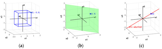
Figure 9.
Abstraction-based solving process in search space. (a) Search space of , (b) search space of , and (c) search space of .
Then, using the line , we partition , obtaining , as shown in Figure 9c.
Ultimately, the solution is found at the point .
For assignment-based algorithms, unit propagation is a particularly important strategy. Unit propagation significantly reduces the time spent using the most straightforward backtracking methods [11]. Therefore, abstraction also needs a corresponding strategy to reduce the solving time.
The core of unit propagation involves handling the literals after assignment, ensuring that these literals are true in the formula [10,35]. Similarly, abstraction has a similar process for handling these literals. In all literals, abstraction ensures that all positive literals and negative literals are distinct from each other, while making positive literals equal to each other and negative literals equal to each other. That is to say, if a formula contains , then and .
Since abstraction-based sequential solving is also structured as a tree, abstraction-based parallel solving follows the same implementation approach as assignment-based solving: simultaneously checking multiple subtrees. This will not be further elaborated upon here.
4.2. Hybrid Solving
As seen in the previous section, the abstraction-based solving algorithm ultimately divides variables into two categories, resulting in classifications. Therefore, without appropriate strategy optimization, its worst-case time complexity should be . Its search tree, like that of assignment-based solving, is also a full binary tree. However, the assignment-based approach has already developed many pruning strategies. In the current mature state of assignment-based solving methods, revisiting pruning strategies for abstraction is a cumbersome task. Therefore, a more important approach is to combine the two solving methods.
Although the two methods partition the search space differently, the content within the partitioned search space is the same. In fact, the distribution of solutions within the search space changes, but it still maintains the solutions’ form . Therefore, after partitioning the search space using one method, it is still possible to attempt the other method to further partition the search space.
It is worth noting that in assignment-based solving algorithms, the strategy for selecting decision variables, such as VSIDS, plays an important role in the solving time. Some researchers have proven this [36]. Therefore, different strategies for variable selection are also expected to have different impacts on hybrid solving methods.
Thus, we conducted the following experiment:
- Generate a random CNF formula with 350 variables and 4.2 times the number of variables for the number of clauses;
- Use abstraction on variables from randomly selected clauses of length-2 to partition the search space into two parts, referred to as Space R1 and Space R2;
- Use the two most frequently occurring variables in pairs for abstraction to partition the search space into two parts, referred to as Space F1 and Space F2;
- Solve the four search spaces, as well as the original formula, using Minisat;
- Statistical solving times are organized in the table, as shown in Table 7.
Table 7. Solving times for different search spaces with Minisat solver (in seconds).
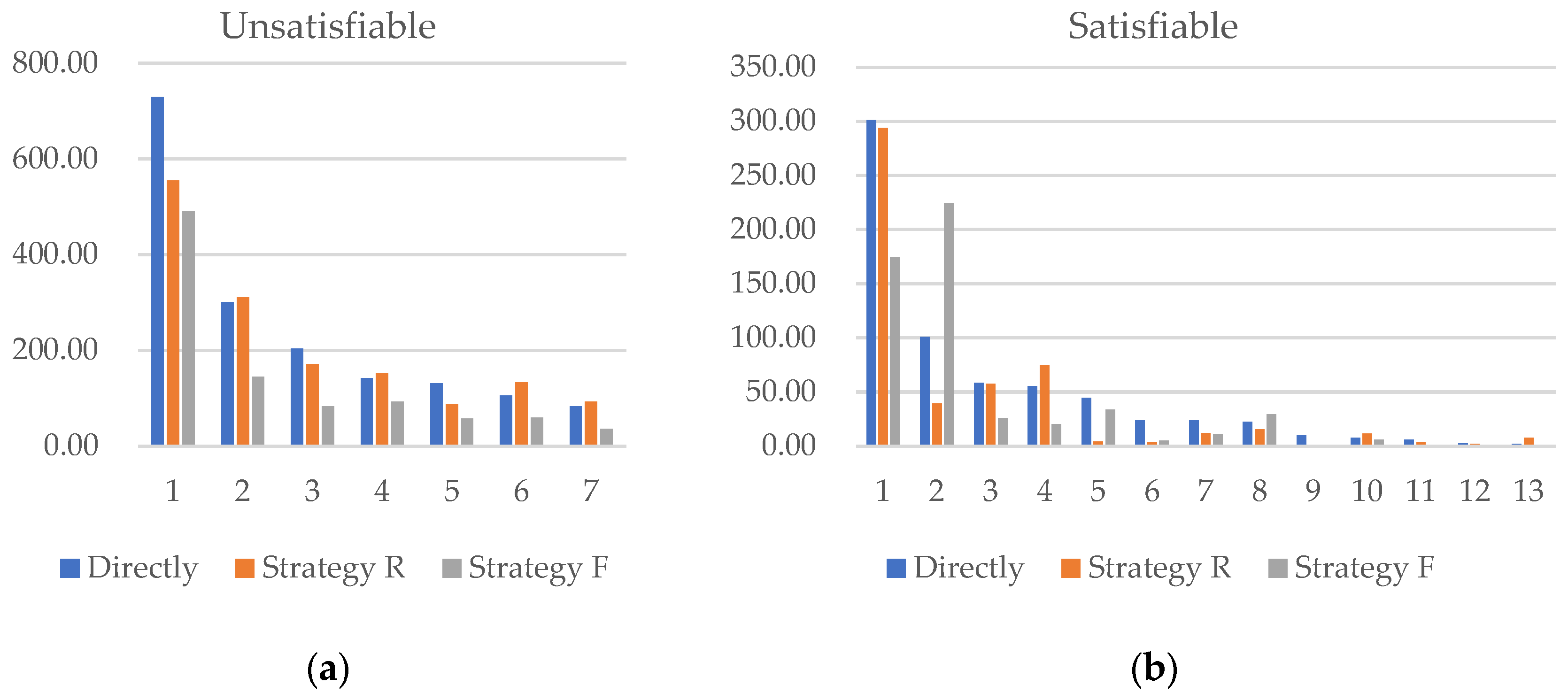
If the two search spaces partitioned through abstraction are solved using a simple DAC parallel solving approach, then when the formula is satisfiable, the solving time should be the minimum value from the two search spaces. When the formula is unsatisfiable, the solving time should be the maximum value from the two search spaces. The impact of different strategies on the solving time is shown in Figure 10.
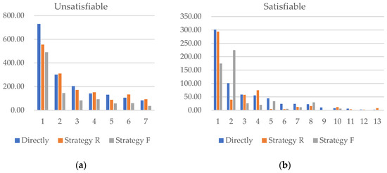
Figure 10.
Comparison of solving times between DAC parallel strategies and direct solving. (a) Time comparison when the formula is unsatisfiable, (b) time comparison when the formula is satisfiable.
It can be observed that, when the formula is satisfiable, Strategy R tends to accelerate solving. When the formula is unsatisfiable, Strategy F is more effective in speeding up the solving process. In addition to the samples above, the experiment calculated a total of 100 CNF formulas, 38 of which are unsatisfiable. In 81% of these cases, Strategy F accelerated solving; for the remaining 62 formulas, Strategy R accelerated solving in 72% of cases. Considering that this is a simple parallel method, the probability of improving computational efficiency should be higher in more advanced parallel algorithms.
To examine the impact of the number of variables or clauses on abstract hybrid solving, we controlled the number of variables or clauses while changing the other factor. The results are shown in Appendix A.1. The solver used in the above experiments is MiniSat. To investigate the impact of abstraction on different solvers, we also tested other solvers, with the test data sourced from SAT competition 2024. The data obtained from these tests are shown in Appendix A.2.
All these experiments led to a similar conclusion: abstract hybrid solving can optimize solving time in most cases.
Analyzing the reason behind this, we believe that the main factor is that abstraction alters the length of certain clauses. This affects the unit propagation process, which, as emphasized earlier, is crucial for solving performance [10].
If Strategy R is used, where variables in length-2 clauses are abstracted, single literals are produced, allowing unit propagation to occur. If Strategy F is used, where the most frequently occurring variable pairs are selected for abstraction, clauses that were originally length-3 become length-2, enabling unit propagation in a process where it would otherwise be impossible.
Take formula as an example, abstraction is applied using two strategies. From Figure 11, it can be observed that in Strategy R, the new clause produced by abstraction participates in the unit propagation process. In Strategy F, the original clause changes from to , allowing clause to determine the variable assignments in through unit propagation, continuing the influence of unit propagation.
Figure 11.
The impact of different strategies on unit propagation. (a) Formula after abstraction using Strategy R and the unit propagation path, (b) formula after abstraction using Strategy F and the unit propagation path.
Similarly, both strategies can lead to the removal of clauses directly from the formula, and these removed clauses might have participated in unit propagation in the original assignment-based solving algorithm.
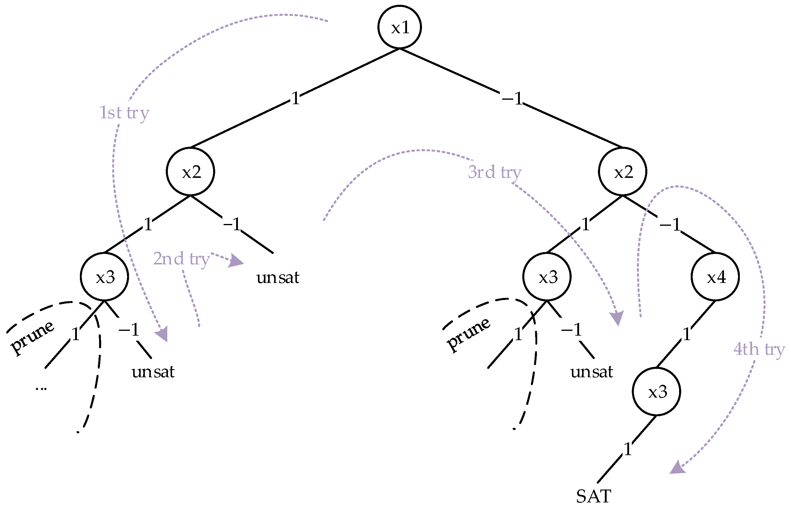
One of the other effects of reducing clause length is its impact on backtracking. For example, consider the following formula:
When solving this formula using the assignment-based method, four backtrack operations are performed, and the paths are shown in Figure 12.
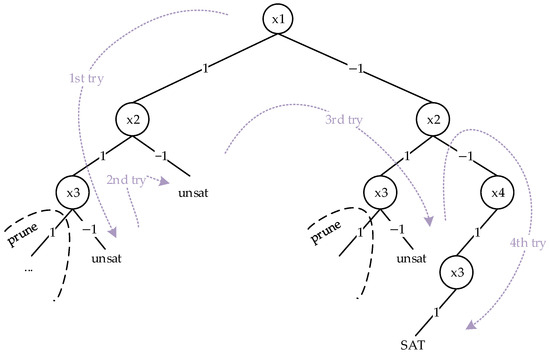
Figure 12.
Backtracking paths when solving formula directly.
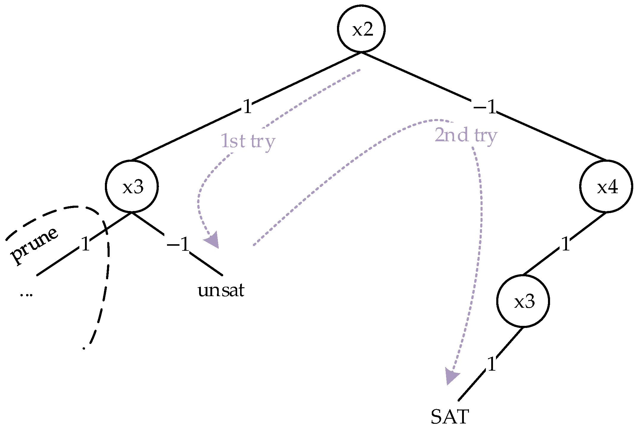
If we first perform abstraction on the formula, we obtain the following:
As shown in Figure 13, when solving the abstracted formula using the assignment-based method, only two backtrack operations are performed, and the depth of each backtrack is not deep.
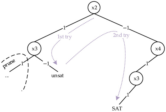
Figure 13.
Backtracking paths after abstraction of formula followed by solving.
As mentioned in Section 2.1, backtracking determines how to retreat during the search, while unit propagation primarily determines how to advance the search. Abstraction impacts both of these processes, causing some calculations to speed up and others to slow down in algorithms that combine abstraction and assignment. Therefore, compared to DAC, it might be more worthwhile to try incorporating abstraction as a new strategy into portfolio-based parallel solving methods.
Additionally, abstraction can also be useful in SMTs (Satisfiability Modulo Theories) [37]. SMTs refer to more complex constraint problems that build on traditional SAT problems by introducing additional theoretical constraints, such as arithmetic, strings, and matrices, etc. [37,38,39]. As a result, solving SMT problems is divided into two parts: the SAT solver and the theory solver, often referred to as DPLL(T) [40].
The SAT solver is used to obtain feasible atomic assignments, while the theory solver checks these atomic assignments. If they are not feasible, the theory solver feeds back to the SAT solver for further adjustments.
For example, consider the expression
In SMTs, these details are initially ignored, and the formula is treated as a propositional formula The solver first solves it, for instance by assigning and , and then passes these assignments to the theory solver to check if they satisfy the constraints. This means checking if holds, and simultaneously ensuring that also holds. If the assignments do not satisfy the constraints, the theory solver returns , and the SAT solver continues the search. This iterative process continues until a solution is found.
The abstraction proposed in this paper is actually based on atomic equivalence relations, such as or . From the perspective of abstraction, whether certain variables are equal or not can simplify the formula. In the formula and , it is clear that they cannot both hold simultaneously. Therefore, we can conclude that , which allows for the further simplification of the formula. This approach can also be used to assess the satisfiability of SMT problems using abstraction.
In other words, through the theory solver, we can pre-determine the equivalence of certain atoms. By integrating abstraction into the SMT solver, we can simplify the formula based on these equivalences before continuing with the solving process.
4.3. Summary of Abstraction-Based Solving
In the previous section, we explained step by step how the abstraction-based SAT solving algorithm is implemented. In this subsection, we will briefly review the entire solving process and highlight the differences between it and the assignment-based solving approach.
Compared to traditional assignment-based solving, the main difference with abstraction-based solving is that it does not assign values to propositional atoms. Instead, it classifies the propositional atoms. If we continued abstraction to its extreme, where all atoms are classified into two categories, it would essentially become a purely abstraction-based algorithm. However, if abstraction is carried out to a certain extent and then an assignment-based algorithm is used, it becomes a hybrid solving method. As shown in Figure 14, the relationship between the two approaches is clear.
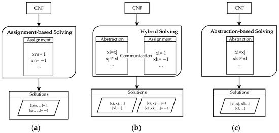
Figure 14.
Differences between assignment-based and abstraction-based solving. (a) Solving with just assignment, (b) solving with abstraction and assignment, and (c) solving with just abstraction.
As shown in Figure 14a, when only using the assignment-based solving method, the result will be the variable assignments. If only the abstraction-based solving method is used, the result will be two sets of different variables, as depicted in Figure 14c. However, when using the hybrid solving method, the result will include both the two sets of different variables and the assignments of certain elements within those sets, as shown in Figure 14b.
So far, we have outlined the specific methods and implementation steps for abstraction, as well as its potential benefits. However, during our actual solutions, we still encountered some issues.
Although the experimental data suggest that abstract hybrid solving can accelerate the solving process in most cases, they also indicate that in certain situations, the efficiency of abstract hybrid assignment solving is not as good as when directly using assignment-based solving. In fact, the time consumed may even be significantly higher than that of direct solving.
As mentioned in the experiments, the selection of abstract variables plays a crucial role in the solving process. However, to date, there is no optimal strategy for choosing variables for abstraction. The two strategies used in the experiments are among the simplest and most straightforward.
Additionally, the experiments were conducted by first performing abstraction just once and then solving. How to integrate abstraction with the existing solvers and establishing communication between the two methods are areas that require further research.
Finally, the method still lacks the corresponding strategies when dealing with large-scale problems, as the cost of certain abstraction strategies, such as identifying the most frequent pairs of variables, increases with problem size.
5. Unified Method for Search Space Partitioning
Below, we have listed the logical expressions for solving based on assignment and abstraction:
Assignment: .
Abstraction: .
The logical formulas and represent a partition of the search space, while their counterparts and are complementary partitions. As we mentioned in Section 3.3, Formula (9): .
If we simplify the formula, we obtain , which simplifies to , thus demonstrating that satisfiability entirely depends on the formula .
In fact, we can give a unified definition for such a partition of the search space.
Definition 4.
Given a formula , if , , …, are logical partitions of respectively, then , , …, are called a set of logical partitions of . is called the partition formula, and is called the subpartition formula. If , then , , …, are called a set of complete logical partitions of .
From Proposition 1, it is known that, regardless of whether a set of partitions is complete, as long as there is a solution in any partition, the original formula must have a solution.
Theorem 1.
If , , …, are a set of logical partitions of , and the partition formula is satisfiable, then is satisfiable.
Theorem 1 only guarantees the sufficiency that if the partition formula is satisfiable, then the original formula is satisfiable. The advantage of a complete partition is that it not only provides the necessary condition, but also shows the situation where the original formula has no solution.
Theorem 2.
If , , …, are a set of complete logical partitions of , then is unsatisfiable if and only if the partition formula is unsatisfiable, and is satisfiable if and only if the partition formula is satisfiable.
Proof.
Let the set of partitions be , , …, , and let .
The partition formula is as follows:
- 1.
- Consistency of Unsatisfiability:
Sufficiency: If is unsatisfiable, since it is a set of complete partitions, . Thus, is unsatisfiable. Therefore, is unsatisfiable, i.e., for any , is unsatisfiable.
Necessity: If for any , is unsatisfiable, the partition formula is unsatisfiable. Hence, is unsatisfiable, since . Therefore, is unsatisfiable.
- 2.
- Consistency of Satisfiability:
Sufficiency: If is satisfiable, since , then . Therefore, is satisfiable. Hence, there exists some such that is satisfiable, which implies that if is satisfiable, the partition formula is satisfiable.
Necessity: If the partition formula is satisfiable, this is equivalent to Theorem 1. □
At the same time, when describing the partitions based on assignment and abstraction, we mentioned that the two partitions are composed of complementary formulas. If we make a strict definition, we can further formalize the partitions.
Definition 5.
Given a formula , if , , …, are logical partitions of , then , , …, are called a set of logical partitions of , is called the partition formula, and is called the subpartition formula. If for any and , , then , , …, are called a set of independent logical partitions of .
The completeness of the partitions ensures that this set of partitions can reveal the satisfiability of the formula, while the independence of the partitions helps identify which partition the solution falls into when the formula is satisfiable.
Theorem 3.
If , , …, are a set of independent complete logical partitions of , and is satisfiable, then for every solution , there exists exactly one logical subpartition such that the subpartition formula .
Proof.
Let the set of partitions be , , …, , and let , a solution .
The partition formula is as follows:
From completeness, we know that .
Thus, . Therefore, is satisfiable and there exists some such that ) = 1.
Now, assume that another subpartition exists, such that .
Therefore, . Thus, .
From the independence of the partitions, we know that , which leads to a contradiction. Therefore, there can only exist one subpartition , such that the subpartition formula is satisfiable. □
According to the pigeonhole principle, we know that for any three Boolean variables, there must be two variables with the same assignment. That is,
If we consider these three logical formulas as a set of logical partitions, then this set of partitions is complete, and its partition formula is as follows:
However, the conjunction of any two logical partitions is satisfiable, meaning that they are not independent logical partitions. When solving the first search space, solutions in other search spaces will repeat previously verified solutions. For example, when searching the space of , some solutions satisfying will also be searched.
From the search space, we can see that, for example, in three dimensions, the planes , , will all pass through the line in the space. This line may contain some solutions, causing the search on each plane to repeatedly verify these assignments.
In contrast, in the assignment-based partition, each plane does not intersect, and is thus independent. In the abstraction-based partition, since each plane intersects at the coordinate axes, and no points from the search space lie on the axes, this partition is also independent.
In some local search algorithms, the algorithm assigns values to multiple variables at once [41,42]. If we use partitions, this form can be represented by the following logical formula:
where represents one term of the Principal Disjunctive Normal Form (PDNF) constructed from , and it, along with the other terms of this PDNF, forms a set of independent complete logical partitions of . Independence ensures that the assignments already checked do not need to be checked again, while completeness guarantees that the satisfiability of the formula can eventually be determined.
Assuming that , this partition divides the search space into equally sized search spaces. checks only one of these, while contains the remaining search spaces. By flipping a literal in , we obtain a term from . From Theorem 2, it can be deduced that to determine satisfiability, each remaining search space must be checked individually, which requires exponential time. Therefore, local search algorithms often flip certain variables based on the satisfiability of clauses [36,43], meaning that they selectively solve within the remaining search space.
In addition, in parallel SAT algorithms, there is another type of search space partition called XOR partition [10,43].
This partition is also independent and complete, and it is equivalent to the abstraction-based partition when there are only two variables.
Through analysis of the partitions, we can conclude that, in addition to mixing abstraction-based and assignment-based solving, different solving algorithms can also be combined, as long as the partitions they correspond to are independent and complete. This ensures both consistency between the satisfiability of all search spaces and the satisfiability of the original formula, while avoiding redundant calculations.
6. Conclusions
This paper analyzes the solving process of the SAT problem from the perspective of search space. It defines the search space and its partitioning from both topological and logical perspectives, and explains their relationship: logical partitions can be represented as certain hyperplanes in a topological space. This conclusion connects the geometric meaning of SAT problem solving in topological spaces with logical operators and may provide a different perspective for solving the SAT problem.
The paper then analyzes the search space partitioning in assignment-based solving and proposes a new search space partitioning method, called abstraction. Using the steps of assignment-based solving as a reference, the steps for abstraction-based solving and their hybrid solving process are defined. Experimental data show that hybrid solving using both abstraction and assignment can accelerate solving in most cases. By combining more different search space partitions and studying the situations that are suitable for these partitions, a new direction can be provided for improving the efficiency of SAT problem solving.
Finally, the paper also presents a unified method for search space partitioning, defining the meanings of independent partitions and complete partitions, and explaining how some existing algorithms perform partitioning. This demonstrates that search space partitioning is, in fact, an effective method for improving the efficiency of SAT problem solving.
In future work, one key area to focus on is researching suitable abstraction strategies that can significantly reduce solving time and cope with large-scale problems. As mentioned earlier, combining abstraction with assignment-based solving is worth exploring more than directly using abstraction alone. Therefore, another important aspect is to study how to integrate abstraction and assignment, developing a solving strategy that can automatically determine when to use assignment-based simplification and when to use abstraction-based simplification, and then implement a corresponding solver.
Author Contributions
Conceptualization, Y.H.; Methodology, Q.N.; Software, Y.H.; Validation, Y.S.; Formal analysis, Y.H.; Investigation, Y.S.; Writing—original draft, Y.H.; Writing—review & editing, Y.S.; Visualization, Y.H.; Supervision, Q.N.; Project administration, Q.N.; Funding acquisition, Q.N. All authors have read and agreed to the published version of the manuscript.
Funding
This research was funded on intelligent classification of emotion states based on co-computing of expression and eye movement (No. 61906051). And The APC was funded by National Natural Science Foundation of China.
Data Availability Statement
The original contributions presented in this study are included in the article. Further inquiries can be directed to the corresponding author.
Conflicts of Interest
The authors declare no conflict of interest.
Appendix A
Appendix A.1
In this experiment, MiniSAT was used to conduct control variable experiments by adjusting the number of propositional atoms and clauses. For each group of experiments, 50 random CNF formulas were generated. Each formula was first simplified using two abstraction strategies, and the minimum time for a successful solution was obtained. This time was then compared with the time taken for direct solving without abstraction. In the data charts, the vertical axis represents the proportion of instances that benefit from acceleration through abstraction.
When the number of variables is 350 and the number of clauses ranges from 3.9 times to 4.5 times the number of variables, the statistical results of abstraction-based hybrid solving efficiency are shown in Figure A1a.
When the number of clauses is 4.2 times the number of variables and the number of variables ranges from 200 to 400, the statistical results of abstraction-based hybrid solving efficiency are shown in Figure A1b.
Analysis of the data shows that abstraction-based hybrid solving can accelerate the solving process in approximately 70% of cases on average. However, we are currently unable to determine the relationship between acceleration and the number of variables or clauses, which may be related to the randomness of the formulas. We will investigate the reasons behind this phenomenon in future work.
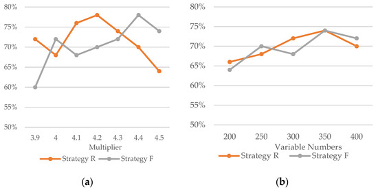
Figure A1.
The proportion of instances where abstraction led to optimized time for 50 instances. (a) Fixed number of variables, different clause multipliers, (b) fixed clause multiplier, different numbers of variables.
Figure A1.
The proportion of instances where abstraction led to optimized time for 50 instances. (a) Fixed number of variables, different clause multipliers, (b) fixed clause multiplier, different numbers of variables.
Appendix A.2
In this experiment, 20 instances from the SAT competition 2024 were selected for solving. The efficiency of abstraction applied to Cadical, Minisat, Glucose, and Maplesat was compared. In Table A1, the solving times for five instances across the four solvers are shown. Solvers marked with the superscript ‘Abst’ indicate that abstraction was applied for simplification before solving, as described in Appendix A.1.
Table A1.
Comparison of solving times before and after applying abstraction for different solvers (in seconds).
Table A1.
Comparison of solving times before and after applying abstraction for different solvers (in seconds).
| Solvers | Instances | ||||
|---|---|---|---|---|---|
| Satisfiable | Unsatisfiable | ||||
| Cadical | 13.64 | 103.11 | 12.21 | 24.60 | 43.62 |
| CadicalAbst | 63.71 | 23.86 | 1.22 | 25.63 | 43.12 |
| Minisat | 3240.12 | 3.73 | 129.72 | 31.08 | 128.60 |
| MinisatAbst | 1616.63 | 8.49 | 131.12 | 29.43 | 117.98 |
| Glucose | 47.42 | 180.71 | 480.86 | 44.33 | 69.05 |
| GlucoseAbst | 198.85 | 0.01 | 228.68 | 39.64 | 65.35 |
| Maplesat | 315.23 | 0.56 | 47.00 | 36.97 | 61.92 |
| MaplesatAbst | 74.87 | 28.91 | 46.82 | 34.54 | 63.65 |
From the data in the table, it can be observed that when the instances are unsatisfiable, the time optimization is not significant. However, when examining the data for the first and second satisfiable instances of Glucose, it is found that while the optimization is sometimes substantial, it can also be slower than direct solving in some cases. Therefore, we calculated the proportion of successful optimization times and the average optimization time for 12 satisfiable and 8 unsatisfiable instances, as shown in Table A2 and Table A3.
Table A2.
Optimization results for satisfiable instances.
Table A2.
Optimization results for satisfiable instances.
| Solver | Optimized | Failed Optimizations | Average Optimized Time |
|---|---|---|---|
| Cadical | 8 | 4 | 16.93 |
| Minisat | 9 | 3 | 345.92 |
| Glucose | 8 | 4 | 51.97 |
| Maplesat | 7 | 5 | 32.58 |
Table A3.
Optimization results for unsatisfiable instances.
Table A3.
Optimization results for unsatisfiable instances.
| Solver | Optimized | Failed Optimizations | Average Optimized Time |
|---|---|---|---|
| Cadical | 4 | 4 | 7.82 |
| Minisat | 5 | 3 | 4.15 |
| Glucose | 4 | 4 | 12.77 |
| Maplesat | 3 | 5 | −3.36 1 |
1 A negative value indicates that the solving time after applying abstraction is higher than the direct solving time.
References
- Cook, S.A. The complexity of theorem-proving procedures. In Logic, Automata, and Computational Complexity: The Works of Stephen A. Cook; Association for Computing Machinery: New York, NY, USA, 2023; pp. 143–152. [Google Scholar]
- Lipparini, E.; Ratschan, S. Satisfiability of non-linear transcendental arithmetic as a certificate search problem. J. Autom. Reason. 2025, 69, 3. [Google Scholar] [CrossRef]
- Ge, N.; Jenn, E.; Breton, N.; Fonteneau, Y. Integrated formal verification of safety-critical software. Int. J. Softw. Tools Technol. Transf. 2018, 20, 423–440. [Google Scholar] [CrossRef]
- Kilani, Y.; Bsoul, M.; Alsarhan, A.; Al-Khasawneh, A. A survey of the satisfiability-problems solving algorithms. J. Intell. Fuzzy Syst. 2023, 45, 445–461. [Google Scholar] [CrossRef]
- Li, C.M.; Xu, Z.; Coll, J.; Manyà, F.; Habet, D.; He, K. Boosting branch-and-bound MaxSAT solvers with clause learning. AI Commun. 2022, 35, 131–151. [Google Scholar] [CrossRef]
- Yang, L.; Wang, X.; Ding, H.; Yang, Y.; Zhao, X.; Pang, L. A survey of intelligent optimization algorithms for solving satisfiability problems. J. Intell. Fuzzy Syst. 2023, 45, 445–461. [Google Scholar] [CrossRef]
- Blanchette, J.C.; Fleury, M.; Lammich, P.; Weidenbach, C. A verified SAT solver framework with learn, forget, restart, and incrementality. J. Autom. Reason. 2018, 61, 333–365. [Google Scholar] [CrossRef]
- Doijade, M.M.; Kulkarni, D.B. Overview of sequential and parallel SAT solvers. In Proceedings of the International Conference on Information Communication and Embedded Systems (ICICES2014), Chennai, India, 27–28 February 2014. [Google Scholar]
- Nair, A.; Chattopadhyay, S.; Wu, H.; Ozdemir, A.; Barrett, C. Proof-Stitch: Proof Combination for Divide-and-Conquer SAT Solvers. In Proceedings of the FMCAD 2022, Trento, Italy, 17–21 October 2022. [Google Scholar]
- Martins, R.; Manquinho, V.; Lynce, I. An overview of parallel SAT solving. Constraints 2012, 17, 304–347. [Google Scholar] [CrossRef]
- Andrici, C.C.; Ciobâcă, Ș. A Verified Implementation of the DPLL Algorithm in Dafny. Mathematics 2022, 10, 2264. [Google Scholar] [CrossRef]
- Chen, X.; Lei, Z.; Lu, P. Deep Cooperation of Local Search and Unit Propagation Techniques. In Proceedings of the 30th International Conference on Principles and Practice of Constraint Programming (CP 2024), Schloss Dagstuhl–Leibniz-Zentrum für Informatik, Girona, Spain, 2–6 September 2024. [Google Scholar]
- Liu, Z.; Yang, P.; Zhang, L.; Huang, X. DeepCDCL: A CDCL-based Neural Network Verification Framework. In International Symposium on Theoretical Aspects of Software Engineering; Springer Nature: Cham, Switzerland, 2024. [Google Scholar]
- Li, C.M.; Xiao, F.; Luo, M.; Manyà, F.; Lü, Z.; Li, Y. Clause vivification by unit propagation in CDCL SAT solvers. Artif. Intell. 2020, 279, 103197. [Google Scholar] [CrossRef]
- Hamadi, Y.; Jabbour, S.; Sais, L. ManySAT: A parallel SAT solver. J. Satisf. Boolean Model. Comput. 2010, 6, 245–262. [Google Scholar] [CrossRef]
- Balyo, T.; Sanders, P.; Sinz, C. Hordesat: A massively parallel portfolio SAT solver. In Theory and Applications of Satisfiability Testing—SAT 2015: 18th International Conference, Austin, TX, USA, 24–27 September 2015; Proceedings 18; Springer International Publishing: Berlin/Heidelberg, Germany, 2015. [Google Scholar]
- Kottler, S.; Kaufmann, M. A Parallel Portfolio SAT Solver with Lockless Physical Clause Sharing; Universitat Tubingen: Tubingen, Germany, 2011. [Google Scholar]
- Atserias, A.; Fichte, J.K.; Thurley, M. Clause-learning algorithms with many restarts and bounded-width resolution. J. Artif. Intell. Res. 2011, 40, 353–373. [Google Scholar] [CrossRef]
- Le Frioux, L.; Baarir, S.; Sopena, J.; Kordon, F. Modular and efficient divide-and-conquer SAT solver on top of the painless framework. In Tools and Algorithms for the Construction and Analysis of Systems: 25th International Conference, TACAS 2019, Held as Part of the European Joint Conferences on Theory and Practice of Software, ETAPS 2019, Prague, Czech Republic, 6–11 April 2019; Proceedings, Part I 25; Springer International Publishing: Berlin/Heidelberg, Germany, 2019. [Google Scholar]
- Osama, M.; Wijs, A.; Biere, A. SAT solving with GPU accelerated inprocessing. In International Conference on Tools and Algorithms for the Construction and Analysis of Systems; Springer International Publishing: Cham, Switzerland, 2021. [Google Scholar]
- Osama, M.; Wijs, A.; Biere, A. Certified SAT solving with GPU accelerated inprocessing. Form. Methods Syst. Des. 2024, 62, 79–118. [Google Scholar] [CrossRef]
- Hartung, M.; Schintke, F. Learned Clause Minimization in Parallel SAT Solvers. arXiv 2019, arXiv:1908.01624. [Google Scholar]
- Sörensson, N. Minisat 2.2 and Minisat++ 1.1. A Short Description in SAT Race 2010. 2010. Available online: https://citeseerx.ist.psu.edu/document?repid=rep1&type=pdf&doi=e46a90899c7ca924c30983cf4cede5804df7ab7f (accessed on 1 January 2025).
- De Moura, L.; Bjørner, N. Z3: An efficient SMT solver. In International Conference on Tools and Algorithms for the Construction and Analysis of Systems; Springer: Berlin/Heidelberg, Germany, 2008. [Google Scholar]
- Coja-Oghlan, A.; Haqshenas, A.; Hetterich, S. Walksat stalls well below satisfiability. SIAM J. Discret. Math. 2017, 31, 1160–1173. [Google Scholar] [CrossRef]
- Soos, M.; Devriendt, J.; Gocht, S.; Shaw, A.; Meel, K.S. Cryptominisat with ccanr at the sat competition 2020. Sat Compet. 2020, 2020, 27. [Google Scholar]
- Biere, A. PicoSAT essentials. J. Satisf. Boolean Model. Comput. 2008, 4, 75–97. [Google Scholar] [CrossRef]
- Li, M.; Shi, Z.; Lai, Q.; Khan, S.; Cai, S.; Xu, Q. Deepsat: An eda-driven learning framework for sat. arXiv 2022, arXiv:2205.13745. [Google Scholar]
- Wang, P.W.; Donti, P.; Wilder, B.; Kolter, Z. Satnet: Bridging deep learning and logical reasoning using a differentiable satisfiability solver. In Proceedings of the 36th International Conference on Machine Learning, Long Beach, CA, USA, 9–15 June 2019. [Google Scholar]
- Sun, Y.; Ye, F.; Zhang, X.; Huang, S.; Zhang, B.; Wei, K.; Cai, S. Autosat: Automatically optimize sat solvers via large language models. arXiv 2024, arXiv:2402.10705. [Google Scholar]
- Zhang, Z.; Chételat, D.; Cotnareanu, J.; Ghose, A.; Xiao, W.; Zhen, H.L.; Zhang, Y.; Hao, J.; Coates, M.; Yuan, M. Grass: Combining graph neural networks with expert knowledge for sat solver selection. In Proceedings of the 30th ACM SIGKDD Conference on Knowledge Discovery and Data Mining, Barcelona, Spain, 25–29 August 2024. [Google Scholar]
- Jha, P.; Li, Z.; Lu, Z.; Bright, C.; Ganesh, V. Alphamaplesat: An MCTS-based cube-and-conquer SAT solver for hard combinatorial problems. arXiv 2024, arXiv:2401.13770. [Google Scholar]
- Tan, S.; Yu, M.; Python, A.; Shang, Y.; Li, T.; Lu, L.; Yin, J. Hyqsat: A hybrid approach for 3-sat problems by integrating quantum annealer with cdcl. In Proceedings of the 2023 IEEE International Symposium on High-Performance Computer Architecture (HPCA), Montreal, QC, Canada, 25 February–1 March 2023. [Google Scholar]
- Saribatur, Z.G.; Eiter, T. Omission-based abstraction for answer set programs. Theory Pract. Log. Program. 2021, 21, 145–195. [Google Scholar] [CrossRef]
- Cai, S.; Lei, Z. Old techniques in new ways: Clause weighting, unit propagation and hybridization for maximum satisfiability. Artif. Intell. 2020, 287, 103354. [Google Scholar] [CrossRef]
- Su, Y.; Yang, Q.; Ci, Y.; Li, Y.; Bu, T.; Huang, Z. Deeply Optimizing the SAT Solver for the IC3 Algorithm. arXiv 2025, arXiv:2501.18612. [Google Scholar]
- Barrett, C.; Tinelli, C. Satisfiability modulo theories. In Handbook of Model Checking; Springer: Berlin/Heidelberg, Germany, 2018; pp. 305–343. [Google Scholar]
- Liang, T.; Reynolds, A.; Tsiskaridze, N.; Tinelli, C.; Barrett, C.; Deters, M. An efficient SMT solver for string constraints. Form. Methods Syst. Des. 2016, 48, 206–234. [Google Scholar] [CrossRef]
- Mufid, M.S.; Adzkiya, D.; Abate, A. SMT-based reachability analysis of high dimensional interval max-plus linear systems. IEEE Trans. Autom. Control 2021, 67, 2700–2714. [Google Scholar] [CrossRef]
- Nieuwenhuis, R.; Oliveras, A.; Tinelli, C. Solving SAT and SAT modulo theories: From an abstract Davis-Putnam-Logemann-Loveland procedure to DPLL (T). J. ACM (JACM) 2006, 53, 937–977. [Google Scholar] [CrossRef]
- Lourenço, H.R.; Martin, O.C.; Stützle, T. Iterated local search: Framework and applications. In Handbook of Metaheuristics; Springer: Berlin/Heidelberg, Germany, 2019; pp. 129–168. [Google Scholar]
- Silva, J.M.; Sakallah, K.A. GRASP—A new search algorithm for satisfiability. In Proceedings of the International Conference on Computer Aided Design, San Jose, CA, USA, 10–14 November 1996. [Google Scholar]
- Andraschko, B.; Danner, J.; Kreuzer, M. SAT solving using XOR-OR-AND normal forms. Math. Comput. Sci. 2024, 18, 20. [Google Scholar] [CrossRef]


Disclaimer/Publisher’s Note: The statements, opinions and data contained in all publications are solely those of the individual author(s) and contributor(s) and not of MDPI and/or the editor(s). MDPI and/or the editor(s) disclaim responsibility for any injury to people or property resulting from any ideas, methods, instructions or products referred to in the content. |
© 2025 by the authors. Licensee MDPI, Basel, Switzerland. This article is an open access article distributed under the terms and conditions of the Creative Commons Attribution (CC BY) license (https://creativecommons.org/licenses/by/4.0/).