
Shock Propagation and the Geometry of International Trade: The US–China Trade Bipolarity in the Light of Network Science


Abstract
1. Introduction
- Q1: Which countries occupy network positions characterized by a high spreadability of a shock to other countries? In other words, which countries have the greatest potential to spread a shock to other countries?
- Q2: Which countries occupy network positions characterized by a high susceptibility to shocks coming from other countries? In other words, which countries can easily be “infected” by shocks originating from other countries?
- Q3: Which countries are intrinsically robust to exogenous shocks due to their own high domestic production?
- Q4: How well do countries diversify the risk of a demand or supply shock?
2. Methodology
2.1. Data
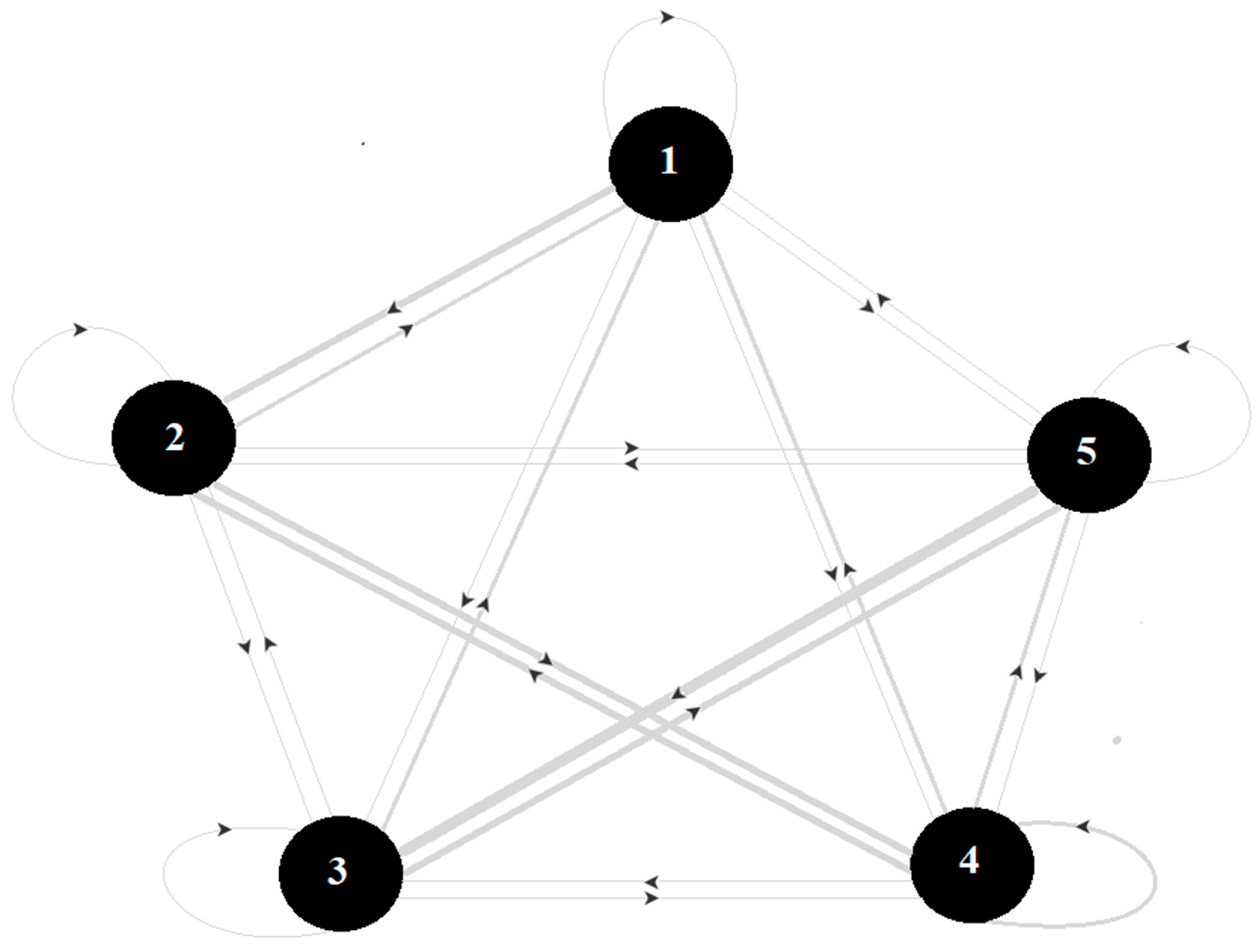
2.2. Modeling International Trade as a Network
2.3. Indicators for the Countries (Analysis at the Micro Level)
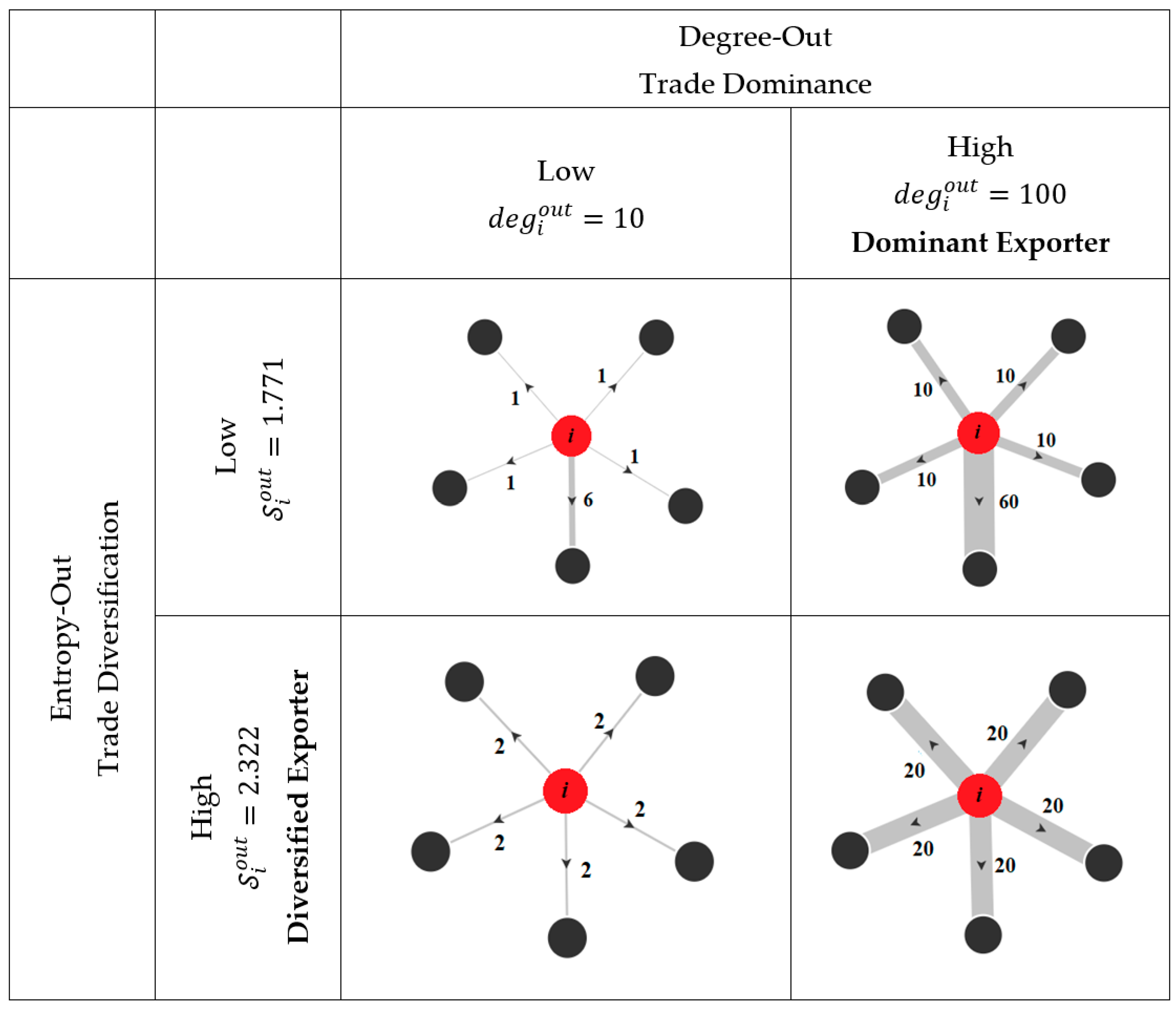
2.3.1. Degree
2.3.2. Balance of Trade
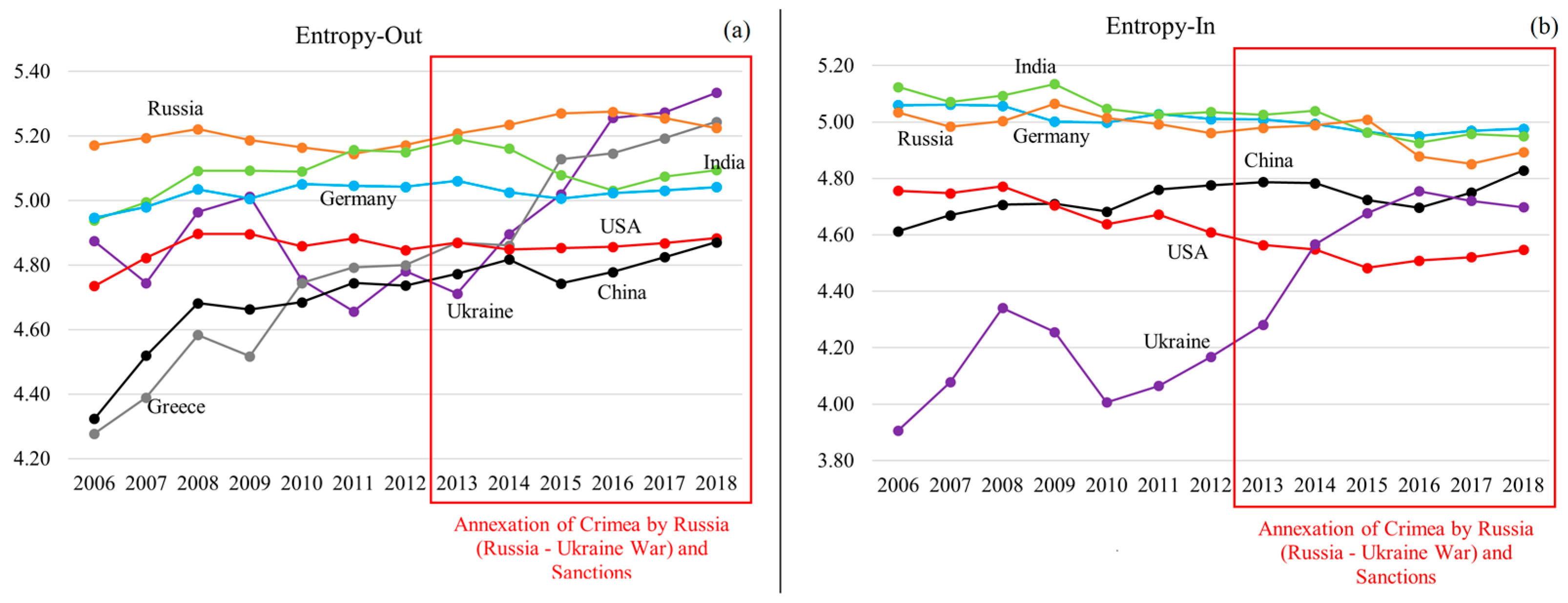
2.3.3. Entropy
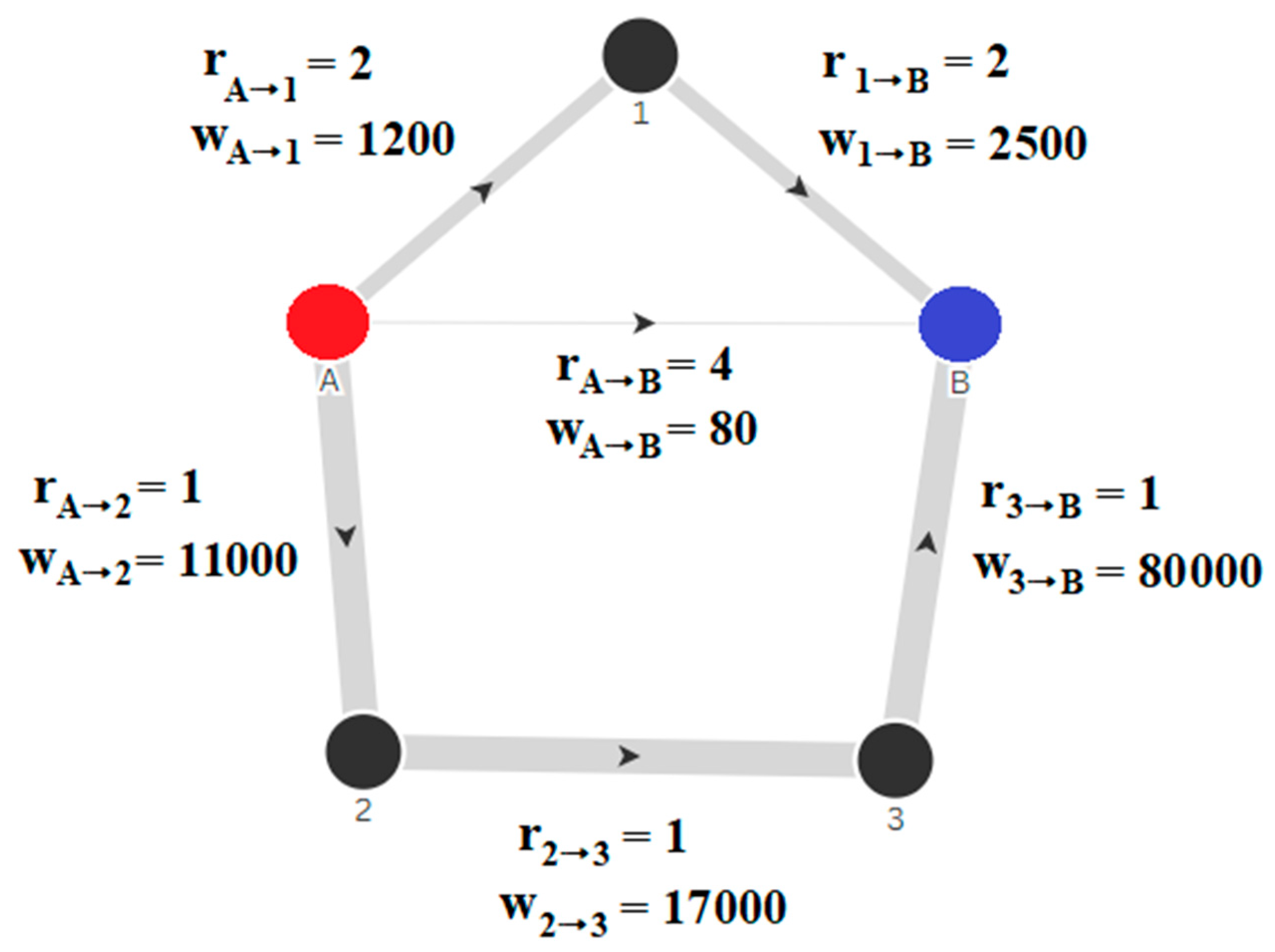
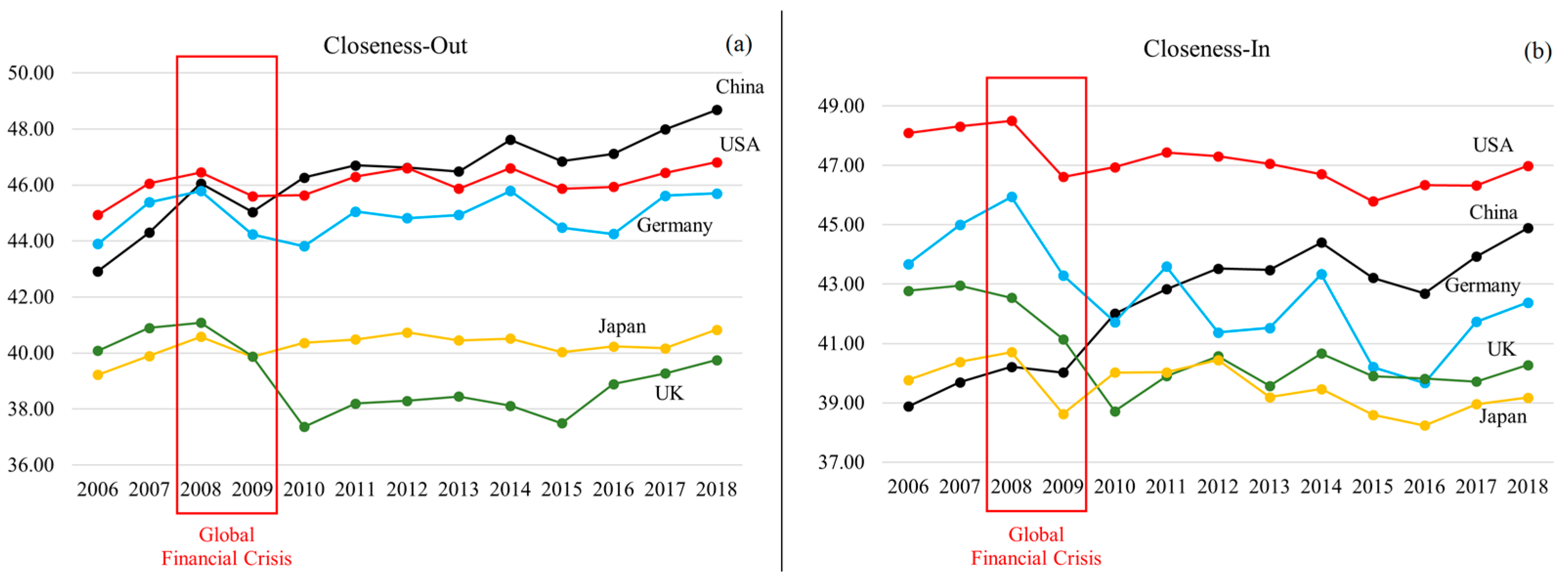
2.3.4. Closeness
2.3.5. Betweenness
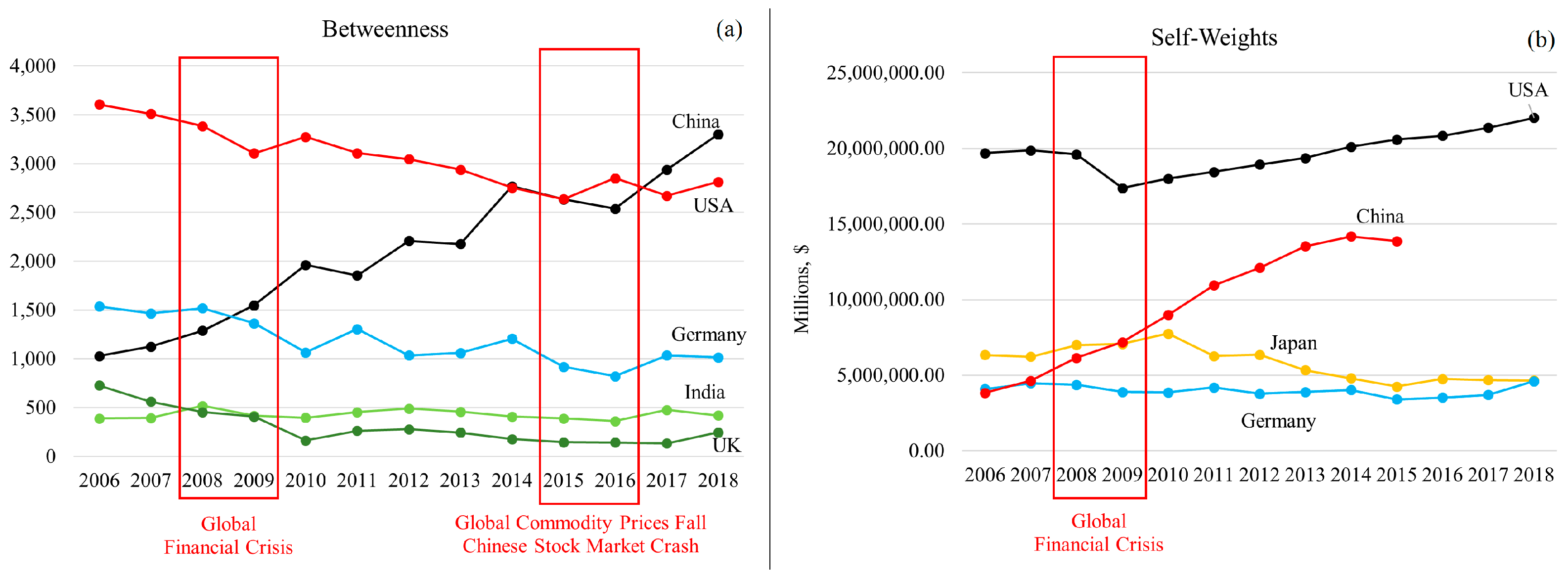
2.3.6. Self-Weights
- A high value of due to relatively high domestic production indicates the high intrinsic robustness of country in the event of an exogenous shock (self-reliant country). Holding everything else constant (ceteris paribus), an exogenous shock which infects country will not largely affect its domestic market due to its own high production.
- A low value of due to relatively low domestic production indicates a low intrinsic robustness of country in the event of an exogenous shock. Holding everything else constant (ceteris paribus), an exogenous shock which infects country will largely affect its domestic market due to its high dependence on foreign markets.
2.4. Indicators for the International Trade Network (Analysis at the Macro Level)
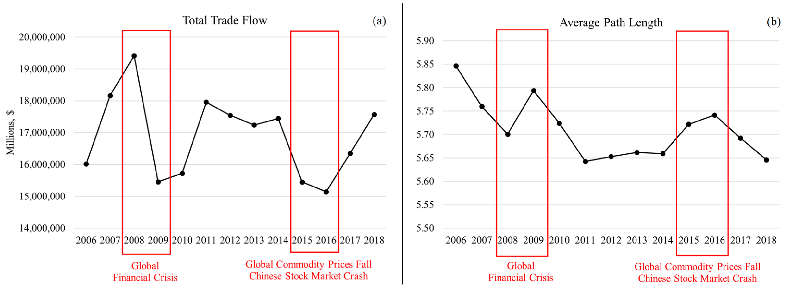
2.4.1. Total Trade Flow
2.4.2. Average Path Length
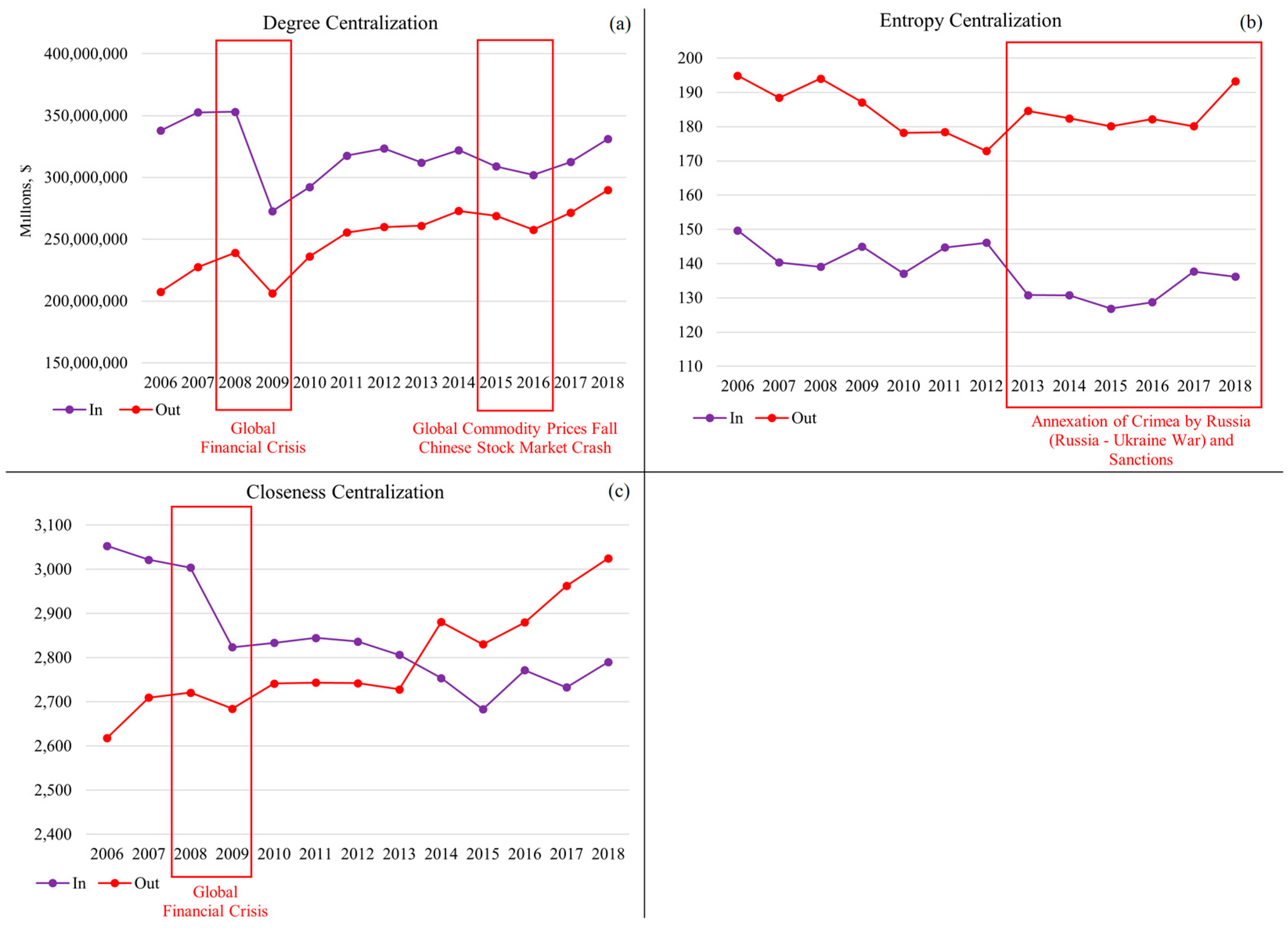
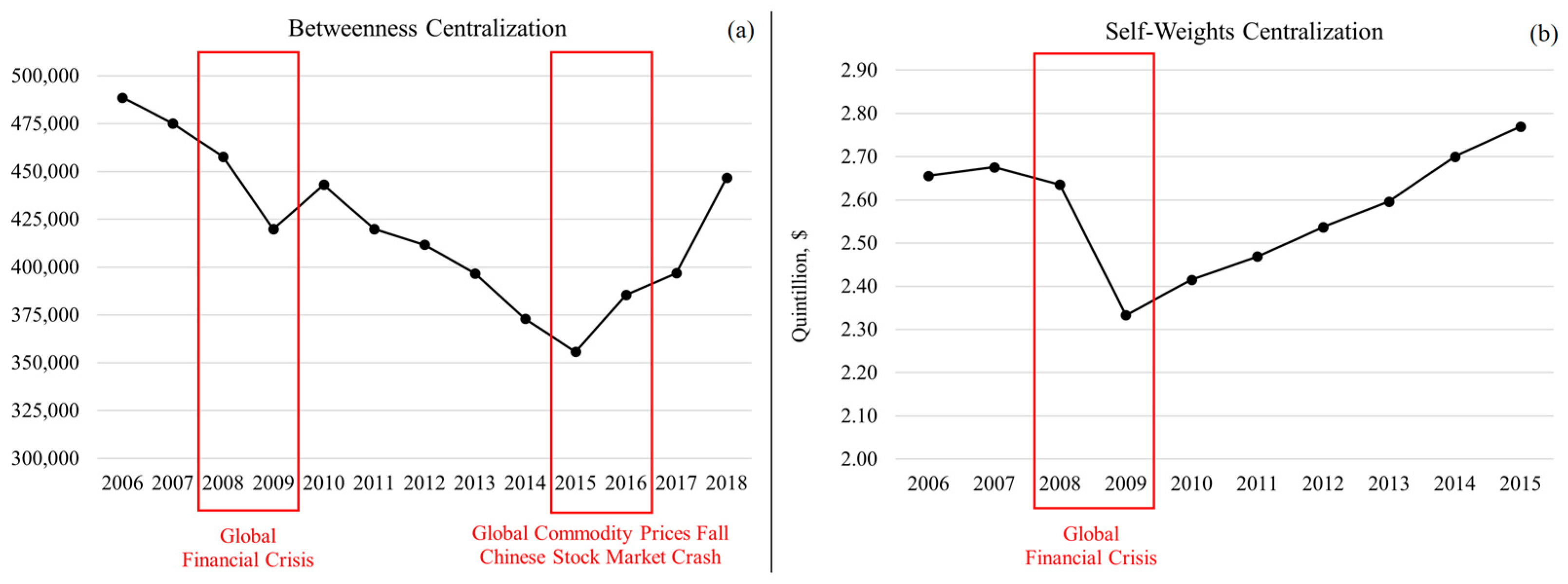
2.4.3. Centralization
3. Results
3.1. Results for the Countries
3.2. Results for the International Trade Network
4. Conclusions
Supplementary Materials
Author Contributions
Funding
Data Availability Statement
Acknowledgments
Conflicts of Interest
Correction Statement
Appendix A
| No. | Country Abbreviation | Country |
| 1 | ALB | Albania |
| 2 | ARM | Armenia |
| 3 | ATG | Antigua and Barbuda |
| 4 | AUS | Australia |
| 5 | AUT | Austria |
| 6 | AZE | Azerbaijan |
| 7 | BDI | Burundi |
| 8 | BEL | Belgium |
| 9 | BFA | Burkina Faso |
| 10 | BGD | Bangladesh |
| 11 | BGR | Bulgaria |
| 12 | BHS | Bahamas |
| 13 | BLR | Belarus |
| 14 | BLZ | Belize |
| 15 | BOL | Bolivia |
| 16 | BRA | Brazil |
| 17 | BRB | Barbados |
| 18 | BRN | Brunei |
| 19 | BTN | Bhutan |
| 20 | BWA | Botswana |
| 21 | CAN | Canada |
| 22 | CHE | Switzerland |
| 23 | CHL | Chile |
| 24 | CHN | China |
| 25 | CIV | Côte d’Ivoire |
| 26 | CMR | Cameroon |
| 27 | COG | Congo |
| 28 | COL | Colombia |
| 29 | CPV | Cape Verde |
| 30 | CRI | Costa Rica |
| 31 | CYP | Cyprus |
| 32 | CZE | Czech Republic |
| 33 | DEU | Germany |
| 34 | DNK | Denmark |
| 35 | DOM | Dominican Republic |
| 36 | DZA | Algeria |
| 37 | ECU | Ecuador |
| 38 | EGY | Egypt |
| 39 | ESP | Spain |
| 40 | EST | Estonia |
| 41 | ETH | Ethiopia |
| 42 | FIN | Finland |
| 43 | FJI | Fiji |
| 44 | FRA | France |
| 45 | GBR | United Kingdom of Great Britain and Northern Ireland |
| 46 | GEO | Georgia |
| 47 | GHA | Ghana |
| 48 | GIN | Guinea |
| 49 | GMB | Gambia |
| 50 | GNB | Guinea-Bissau |
| 51 | GNQ | Equatorial Guinea |
| 52 | GRC | Greece |
| 53 | GUY | Guyana |
| 54 | HKG | Hong Kong |
| 55 | HND | Honduras |
| 56 | HRV | Croatia |
| 57 | HUN | Hungary |
| 58 | IDN | Indonesia |
| 59 | IND | India |
| 60 | IRL | Ireland |
| 61 | IRN | Iran |
| 62 | IRQ | Iraq |
| 63 | ISL | Iceland |
| 64 | ISR | Israel |
| 65 | ITA | Italy |
| 66 | JAM | Jamaica |
| 67 | JOR | Jordan |
| 68 | JPN | Japan |
| 69 | KAZ | Kazakhstan |
| 70 | KEN | Kenya |
| 71 | KGZ | Kyrgyzstan |
| 72 | KHM | Cambodia |
| 73 | KOR | South Korea |
| 74 | KWT | Kuwait |
| 75 | LAO | Laos |
| 76 | LCA | Saint Lucia |
| 77 | LKA | Sri Lanka |
| 78 | LTU | Lithuania |
| 79 | LUX | Luxembourg |
| 80 | LVA | Latvia |
| 81 | MAR | Morocco |
| 82 | MDA | Moldova |
| 83 | MDG | Madagascar |
| 84 | MDV | Maldives |
| 85 | MEX | Mexico |
| 86 | MKD | North Macedonia |
| 87 | MLI | Mali |
| 88 | MLT | Malta |
| 89 | MNG | Mongolia |
| 90 | MOZ | Mozambique |
| 91 | MUS | Mauritius |
| 92 | MWI | Malawi |
| 93 | MYS | Malaysia |
| 94 | NAM | Namibia |
| 95 | NER | Niger |
| 96 | NGA | Nigeria |
| 97 | NIC | Nicaragua |
| 98 | NLD | Netherlands |
| 99 | NOR | Norway |
| 100 | NPL | Nepal |
| 101 | NZL | New Zealand |
| 102 | OMN | Oman |
| 103 | PAK | Pakistan |
| 104 | PAN | Panama |
| 105 | PER | Peru |
| 106 | PHL | Philippines |
| 107 | PNG | Papua New Guinea |
| 108 | POL | Poland |
| 109 | PRT | Portugal |
| 110 | PRY | Paraguay |
| 111 | PSE | Palestine |
| 112 | QAT | Qatar |
| 113 | ROU | Romania |
| 114 | RUS | Russia |
| 115 | RWA | Rwanda |
| 116 | SAU | Saudi Arabia |
| 117 | SEN | Senegal |
| 118 | SGP | Singapore |
| 119 | SLV | El Salvador |
| 120 | SRB | Serbia |
| 121 | SVK | Slovakia |
| 122 | SVN | Slovenia |
| 123 | SWE | Sweden |
| 124 | SWZ | Eswatini |
| 125 | SYC | Seychelles |
| 126 | TGO | Togo |
| 127 | THA | Thailand |
| 128 | TTO | Trinidad and Tobago |
| 129 | TUN | Tunisia |
| 130 | TUR | Turkey |
| 131 | TZA | Tanzania |
| 132 | UKR | Ukraine |
| 133 | URY | Uruguay |
| 134 | USA | United States of America |
| 135 | VNM | Vietnam |
| 136 | VUT | Vanuatu |
| 137 | ZAF | South Africa |
| 138 | ZMB | Zambia |
References
- Fagiolo, G.; Reyes, J.; Schiavo, S. The evolution of the world trade web: A weighted-network analysis. J. Evol. Econ. 2010, 20, 479–514. [Google Scholar] [CrossRef]
- Wang, X.; Ma, L.; Yan, S.; Chen, X.; Growe, A. Trade for food security: The stability of global agricultural trade networks. Foods 2023, 12, 271. [Google Scholar] [CrossRef]
- Zhang, Y.T.; Li, M.Y.; Zhou, W.X. Impact of the Russia-Ukraine conflict on international staple agrifood trade networks. Foods 2024, 13, 2134. [Google Scholar] [CrossRef]
- Papadopoulos, G.D.; Magafas, L.; Demertzis, K.; Antoniou, I. Analyzing global geopolitical stability in terms of world trade network analysis. Information 2023, 14, 442. [Google Scholar] [CrossRef]
- Ma, C.; Zhang, L.; You, L.; Tian, W. A review of supply chain resilience: A network modeling perspective. Appl. Sci. 2024, 15, 265. [Google Scholar] [CrossRef]
- Chang, J.J.; Du, H.; Lou, D.; Polk, C. Ripples into waves: Trade networks, economic activity, and asset prices. J. Financ. Econ. 2022, 145, 217–238. [Google Scholar] [CrossRef]
- Zhu, M.; Dong, P.; Ju, Y.; Fu, Z. Assessing economies’ resilience of international liquefied natural gas trade network in the presence of the ripple effect. Energy 2024, 313, 133491. [Google Scholar] [CrossRef]
- Allen, W.A.; Moessner, R. The international propagation of the financial crisis of 2008 and a comparison with 1931. Financ. Hist. Rev. 2012, 19, 123–147. [Google Scholar] [CrossRef]
- Iloskics, Z.; Sebestyén, T.; Braun, E. Shock propagation channels behind the global economic contagion network: The role of economic sectors and the direction of trade. PLoS ONE 2021, 16, e0258309. [Google Scholar] [CrossRef]
- Parwanto, N.B.; Oyama, T. Investigating the impact of the 2011 Great East Japan Earthquake and evaluating the restoration and reconstruction performance. J. Asian Public Policy 2015, 8, 329–350. [Google Scholar] [CrossRef]
- Dadakas, D.; Pitoňáková, R.; Ioannidis, E. The impact of the Crimea Annexation on Agricultural Trade: A Structural Gravity Approach. Eur. Rev. Agric. Econ. 2025. [Google Scholar] [CrossRef]
- Sampson, T. Brexit: The economics of international disintegration. J. Econ. Perspect. 2017, 31, 163–184. [Google Scholar] [CrossRef]
- Wang, Z. Understanding Trump’s trade policy with China: International pressures meet domestic politics. Pac. Focus 2019, 34, 376–407. [Google Scholar] [CrossRef]
- Lee, Y. Interdependence, issue importance, and the 2009 Russia-Ukraine gas conflict. Energy Policy 2017, 102, 199–209. [Google Scholar] [CrossRef]
- Liu, J.; Li, X. Impact of extreme weather disasters on China’s barley industry under the background of trade friction—Based on the partial equilibrium model. Foods 2022, 11, 1570. [Google Scholar] [CrossRef]
- Freeman, L.C. Centrality in social networks: Conceptual clarification. Soc. Netw. 1978, 1, 215–239. [Google Scholar] [CrossRef]
- Newman, M. Networks: An Introduction; Oxford University Press: Oxford, UK, 2018. [Google Scholar] [CrossRef]
- Shannon, C.E. A mathematical theory of communication. Bell Syst. Tech. J. 1948, 27, 379–423. [Google Scholar] [CrossRef]
- Angelidis, G.; Ioannidis, E.; Makris, G.; Antoniou, I. Competitive conditions in global value chain networks: An assessment using entropy and network analysis. Entropy 2020, 22, 1068. [Google Scholar] [CrossRef]
- Angelidis, G.; Varsakelis, N.C. Economic shock transmission through global value chains: An assessment using network analysis. Int. Adv. Econ. Res. 2023, 29, 111–128. [Google Scholar] [CrossRef]
- Antonietti, R.; Falbo, P.; Fontini, F.; Grassi, R.; Rizzini, G. The world trade network: Country centrality and the COVID-19 pandemic. Appl. Netw. Sci. 2022, 7, 18. [Google Scholar] [CrossRef]
- Amico, A.; Verginer, L.; Casiraghi, G.; Vaccario, G.; Schweitzer, F. Adapting to disruptions: Managing supply chain resilience through product rerouting. Sci. Adv. 2024, 10, eadj1194. [Google Scholar] [CrossRef]
- Na, L.; Minjun, S.; Wen, H. Impacts of the Euro Sovereign Debt Crisis on Global Trade and Economic Growth: A General Equilibrium Analysis Based on GTAP Model. Available online: https://ageconsearch.umn.edu/record/332356/?v=pdf (accessed on 11 September 2024).
- Lee, M.; Park, D.; Abdon, A.; Estrada, G. Economic impact of Eurozone sovereign debt crisis on developing Asia. In Global Banking, Financial Markets and Crises; Emerald Group Publishing Limited: Bingley, UK, 2013; pp. 271–304. [Google Scholar] [CrossRef]
- Valentinyine Endresz, M.; Skudelny, F. Crisis Severity and the International Trade Network. ECB Working Paper No. 1971. Available online: https://ssrn.com/abstract=2898921 (accessed on 11 September 2024).
- Alekhina, V.; Yoshino, N. Impact of World Oil Prices on an Energy Exporting Economy including Monetary Policy. ADBI Working Paper 2018. Available online: https://www.adb.org/sites/default/files/publication/411171/adbi-wp828.pdf (accessed on 11 September 2024).
- Salem, L.B.; Nouira, R.; Saafi, S.; Rault, C. How do oil prices affect GDP and its components? New evidence from a time-varying threshold model. Energy Policy 2024, 190, 114162. [Google Scholar] [CrossRef]
- Ahmed, A.D.; Huo, R. Volatility transmissions across international oil market, commodity futures, and stock markets: Empirical evidence from China. Energy Econ. 2021, 93, 104741. [Google Scholar] [CrossRef]
- Yousaf, I.; Hassan, A. Linkages between crude oil and emerging Asian stock markets: New evidence from the Chinese stock market crash. Financ. Res. Lett. 2019, 31, 207–217. [Google Scholar] [CrossRef]
- Fajgelbaum, P.D.; Khandelwal, A.K. The economic impacts of the US–China trade war. Annu. Rev. Econ. 2022, 14, 205–228. [Google Scholar] [CrossRef]
- United Nations. UN Comtrade Database. Available online: https://comtradeplus.un.org (accessed on 11 September 2024).
- Namatame, A.; Chen, S.H. Agent-based Modeling and Network Dynamics; Oxford University Press: Oxford, UK, 2016. [Google Scholar] [CrossRef]
- Jackson, M.O. Social and Economic Networks; Princeton University Press: Princeton, NJ, USA, 2008; Available online: https://press.princeton.edu/books/paperback/9780691148205/social-and-economic-networks (accessed on 11 September 2024).
- Goyal, S. Networks: An Economics Approach; MIT Press: Cambridge, MA, USA, 2023; Available online: https://mitpress.mit.edu/9780262048033/networks (accessed on 11 September 2024).
- Angelidis, G.; Bratsas, C.; Makris, G.; Ioannidis, E.; Varsakelis, N.C.; Antoniou, I.E. Global value chains of COVID-19 materials: A weighted directed network analysis. Mathematics 2021, 9, 3202. [Google Scholar] [CrossRef]
- Cover, T.M. Elements of Information Theory; John Wiley & Sons: Hoboken, NJ, USA, 1999. [Google Scholar] [CrossRef]
- Opsahl, T.; Agneessens, F.; Skvoretz, J. Node centrality in weighted networks: Generalizing degree and shortest paths. Soc. Netw. 2010, 32, 245–251. [Google Scholar] [CrossRef]
- Goñi, J.; Van Den Heuvel, M.P.; Avena-Koenigsberger, A.; Velez de Mendizabal, N.; Betzel, R.F.; Griffa, A.; Hagmann, P.; Corominas-Murtra, B.; Thiran, J.P.; Sporns, O. Resting-brain functional connectivity predicted by analytic measures of network communication. Proc. Natl. Acad. Sci. USA 2014, 111, 833–838. [Google Scholar] [CrossRef]
- Rochat, Y. Closeness centrality extended to unconnected graphs: The harmonic centrality index. In ASNA; University of Lausanne: Lausanne, Switzerland, 2009; Available online: https://infoscience.epfl.ch/server/api/core/bitstreams/7f3097a0-d7e0-4cd4-a3f3-82673aab1909/content (accessed on 11 September 2024).
- Hao, Y.; Jia, L.; Wang, Y. Robustness of weighted networks with the harmonic closeness against cascading failures. Phys. A Stat. Mech. Its Appl. 2020, 541, 123373. [Google Scholar] [CrossRef]
- Hao, Y.; Wang, Y.; Jia, L.; He, Z. Cascading failures in networks with the harmonic closeness under edge attack strategies. Chaos Solitons Fractals 2020, 135, 109772. [Google Scholar] [CrossRef]
- Hao, Y.; Jia, L.; Wang, Y.; He, Z. Modelling cascading failures in networks with the harmonic closeness. PLoS ONE 2021, 16, e0243801. [Google Scholar] [CrossRef]
- Ioannidis, E.; Tsoumaris, D.; Ntemkas, D.; Sarikeisoglou, I. Correlations of ESG ratings: A signed weighted network analysis. AppliedMath 2022, 2, 638–658. [Google Scholar] [CrossRef]
- Chor, D.; Manova, K. Off the cliff and back? Credit conditions and international trade during the global financial crisis. J. Int. Econ. 2012, 87, 117–133. [Google Scholar] [CrossRef]
- Karabulut, G.; Bilgin, M.H.; Doker, A.C. The relationship between commodity prices and world trade uncertainty. Econ. Anal. Policy 2020, 66, 276–281. [Google Scholar] [CrossRef]
- Biersack, J.; O’lear, S. The geopolitics of Russia’s annexation of Crimea: Narratives, identity, silences, and energy. Eurasian Geogr. Econ. 2014, 55, 247–269. [Google Scholar] [CrossRef]
- Boyko, N.; Nes, K.; Schaefer, K.A. International trade and Ukraine’s pursuit of self-determination. World Econ. 2024, 47, 1460–1477. [Google Scholar] [CrossRef]
- Wang, J. China’s regional trade agreements: The law, geopolitics, and impact on the multilateral trading system. SYBIL 2004, 8, 119. Available online: https://papers.ssrn.com/sol3/papers.cfm?abstract_id=559382 (accessed on 11 September 2024).
- Xing, L.; Dong, X.; Guan, J.; Qiao, X. Betweenness centrality for similarity-weight networks and its application to measuring industrial sectors’ pivotability on the global value chain. Phys. A Stat. Mech. Its Appl. 2019, 516, 19–36. [Google Scholar] [CrossRef]
- Spyropoulos, A.Z.; Bratsas, C.; Makris, G.C.; Ioannidis, E.; Tsiantos, V.; Antoniou, I. Entropy and network centralities as intelligent tools for the investigation of terrorist organizations. Entropy 2021, 23, 1334. [Google Scholar] [CrossRef]
- Spyropoulos, A.Z.; Bratsas, C.; Makris, G.C.; Ioannidis, E.; Tsiantos, V.; Antoniou, I. Investigation of terrorist organizations using intelligent tools: A dynamic network analysis with weighted links. Mathematics 2022, 10, 1092. [Google Scholar] [CrossRef]
- Spyropoulos, A.Z.; Ioannidis, E.; Antoniou, I. Interoperability and targeted attacks on terrorist organizations using intelligent tools from network science. Information 2023, 14, 580. [Google Scholar] [CrossRef]
- Spyropoulos, A. Study of Complex Systems with Tools of Network Theory: Application: Analysis of Networks of Terrorist Organizations. Ph.D. Dissertation, Democritus University of Thrace, Komotini, Greece, May 2024. [Google Scholar] [CrossRef]
- Barabási, A.L.; Albert, R. Emergence of scaling in random networks. Science 1999, 286, 509–512. [Google Scholar] [CrossRef] [PubMed]
- Guan, J.; Li, Y.; Xing, L.; Li, Y.; Liang, G. Closeness centrality for similarity-weight network and its application to measuring industrial sectors’ position on the Global Value Chain. Phys. A Stat. Mech. Its Appl. 2020, 541, 123337. [Google Scholar] [CrossRef]
- Antoniou, I.; Ioannidis, E.; Varsakelis, N. Co-evolutionary complex networks. In Nonequilibrium Thermodynamics and Fluctuation Kinetics: Modern Trends and Open Questions; Brenig, L., Brilliantov, N., Tlidi, M., Eds.; Springer International Publishing: Cham, Switzerland, 2022; pp. 277–302. [Google Scholar] [CrossRef]
- Tsintsaris, D.; Tsompanoglou, M.; Ioannidis, E. Dynamics of social influence and knowledge in networks: Sociophysics models and applications in social trading, behavioral finance, and business. Mathematics 2024, 12, 1141. [Google Scholar] [CrossRef]

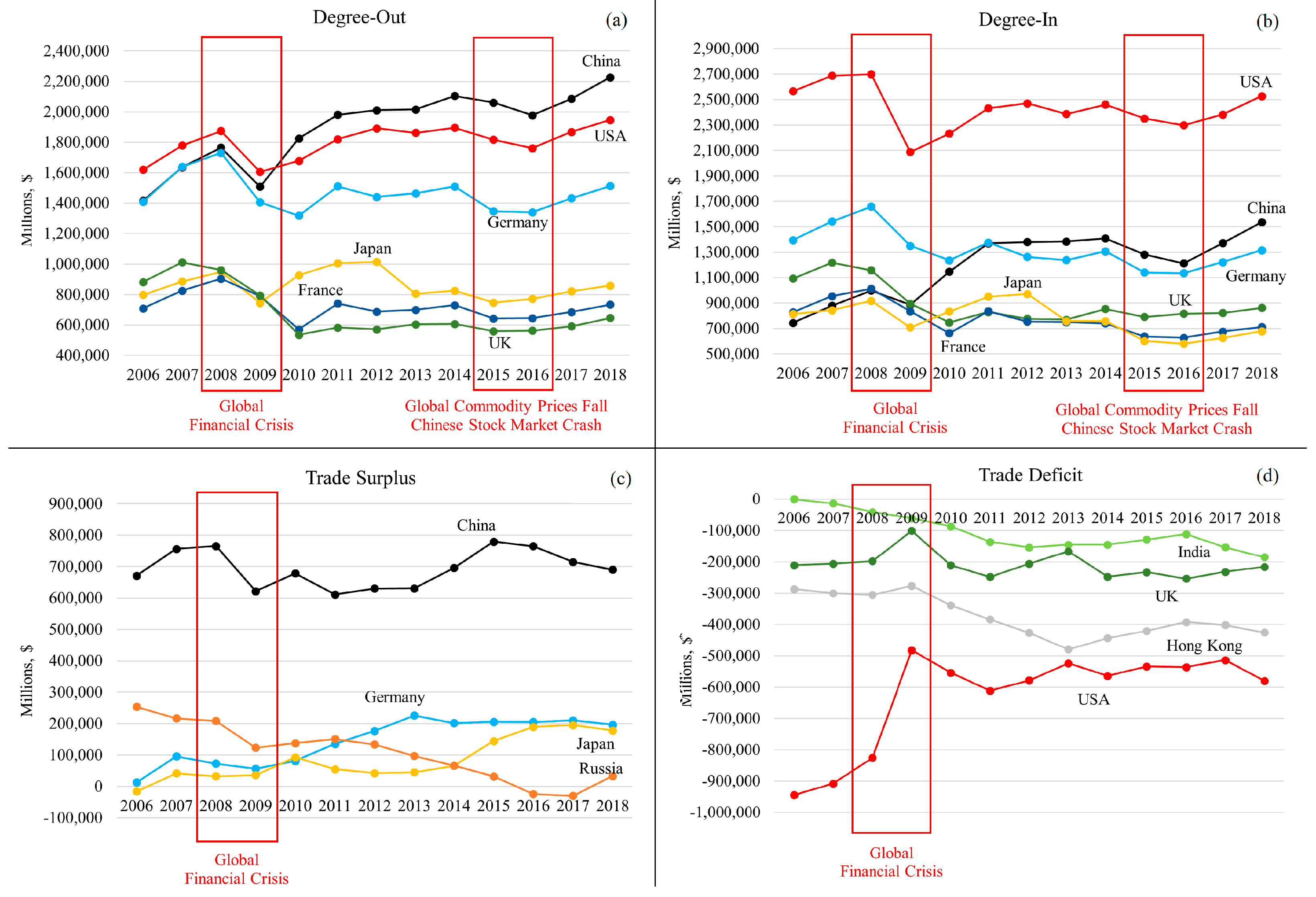
| Year | Event |
|---|---|
| 2008 | Global Financial Crisis [8,9] |
| 2010 | Eurozone Sovereign Debt Crisis [23,24,25] |
| 2014 | Annexation of Crimea by Russia (Russia–Ukraine War) and Sanctions [11] |
| 2015 | Global Fall in Commodity Prices [26,27] |
| 2015 | Chinese Stock Market Crash [28,29] |
| 2016 | Brexit Referendum [12] |
| 2018 | The USA–China Trade War [13,30] |
| Matrix Elements | Notation | Interpretation in the Context of International Trade |
|---|---|---|
| Off-diagonal | Trade flow from country to country | |
| Diagonal self-weights | Domestic production minus exports of country |
| Name | Mathematical Formula | Interpretation in the Context of International Trade |
|---|---|---|
| Degree-Out | The sum of exports from country. A high value indicates a dominant exporter. A dominant exporter has a high spreadability of a shock to its direct trade partners. | |
| Degree-In | The sum of imports to country. A high value indicates a dominant importer. A dominant importer has a high susceptibility to a shock originating from its direct trade partners. |
| Name | Mathematical Formula | Interpretation in the Context of International Trade |
|---|---|---|
| Balance of Trade | If it is positive (negative), then the country has a trade surplus (deficit). A surplus implies that the spreadability of a shock to its direct trade partners is higher compared to the susceptibility to a shock originating from its direct trade partners. Deficit implies the reverse. |
| Name | Mathematical Formula | Interpretation in the Context of International Trade |
|---|---|---|
| Export Distribution | The probability distribution of export trade flows from country . | |
| Import Distribution | The probability distribution of import trade flows to country . | |
| Entropy-Out | The entropy of export trade flows from country. It assesses the diversification of the export trade flows. A high value indicates a diversified exporter. A diversified exporter has low vulnerability to demand shocks in the case where a direct export flow is disrupted. Low value means that country has a portfolio of export trade flows that is mainly concentrated in certain trade partners. | |
| Entropy-In | The entropy of import trade flows to country. It assesses the diversification of the import trade flows. A high value indicates a diversified importer. A diversified importer has low vulnerability to supply shocks in the case where a direct import flow is disrupted. Low value means that country has a portfolio of import trade flows that is mainly concentrated in certain trade partners. |
| IF | THEN |
|---|---|
| Directed Path | Length of the Directed Path Based on: | |
|---|---|---|
| Trade Flow Weights | Shock Resistance Weights | |
| Name | Mathematical Formula | Interpretation in the Context of International Trade |
|---|---|---|
| Distance | The lowest possible sum of resistance weights from country to country, where are the intermediary countries (indirect trade partners). A low value of distance indicates a low resistance to shock propagation from country (source) to country (target). This implies a high spreadability of shock from to, or equivalently, a high susceptibility of to the shock originating from . | |
| Closeness-Out | The sum of inverted export distances from country . A high value indicates a close exporter. A close exporter has a high spreadability of a shock to the whole network, considering not only direct but also indirect trade relationships. | |
| Closeness-In | The sum of inverted import distances to country. A high value indicates a close importer. A close importer has a high susceptibility to a shock originating from the whole network, considering not only direct but also indirect trade relationships. |
| Name | Mathematical Formula | Interpretation in the Context of International Trade |
|---|---|---|
| Betweenness | is the number of shortest directed paths (geodesics) from country to country that pass through the intermediary country. is the number of all shortest directed paths (geodesics) from country to country. A high value means that country plays the role of an intermediary hub, acting as a bridge that favors the further propagation of shocks to other trade clusters or regions of the ITN. |
| Name | Mathematical Formula | Interpretation in the Context of International Trade |
|---|---|---|
| Total Trade Flow | The sum of all trade flows. It assesses the trade dependence among all countries, indicating the density of the ITN. A higher value may contribute to a wider spread of shocks throughout the network. |
| Name | Mathematical Formula | Interpretation in the Context of International Trade |
|---|---|---|
| Average Path Length | Average of all distances . It assesses the average trade distance between two countries, indicating the existence or non-existence of trade lines that act as “shortcuts” in the ITN. A lower value indicates that the countries are closer to each other. This fact may contribute to the further propagation of shocks from one region of the network to another. |
| Name | Mathematical Formula | Interpretation in the Context of International Trade |
|---|---|---|
| Degree-Out Centralization | where | It assesses how dominant the most dominant exporter is in relation to all other countries . A high value means that there are only a few countries that have a much higher spreadability of shock to their direct trade partners compared to the other countries. |
| Degree-In Centralization | where | It assesses how dominant the most dominant importer is in relation to all other countries . A high value means that there are only a few countries that have a much higher susceptibility to a shock originating from their direct trade partners compared to the other countries. |
| Entropy-Out Centralization | where | It assesses how diversified the most diversified exporter is in relation to all other countries. A high value means that there are only a few countries that have a much lower vulnerability to demand shocks (in the case where a direct export flow is disrupted) compared to the other countries. |
| Entropy-In Centralization | where | It assesses how diversified the most diversified importer is in relation to all other countries. A high value means that there are only a few countries that have a much lower vulnerability to supply shocks (in the case where a direct import flow is disrupted) compared to the other countries. |
| Closeness-Out Centralization | where | It assesses how close the closest exporter is in relation to all other countries . A high value means that there are only a few countries that have much higher spreadability of a shock to the whole network (considering not only direct but also indirect trade relationships) compared to the other countries. |
| Closeness-In Centralization | where | It assesses how close the closest importer is in relation to all other countries . A high value means that there are only a few countries that have much higher susceptibility to a shock originating from the whole network (considering not only direct but also indirect trade relationships) compared to the other countries. |
| Betweenness Centralization | where | It assesses how intermediary the most intermediary country is in relation to all other countries . A high value means that there are only a few countries that clearly play the role of an intermediary hub (acting as a bridge between different trade clusters) compared to the other countries. |
| Gross Sales (Self-Weights) Centralization | where | It assesses how self-reliant the most self-reliant country is in relation to all other countries . A high value means that there are only a few countries that have much higher intrinsic robustness to exogenous shocks compared to the other countries. |
Disclaimer/Publisher’s Note: The statements, opinions and data contained in all publications are solely those of the individual author(s) and contributor(s) and not of MDPI and/or the editor(s). MDPI and/or the editor(s) disclaim responsibility for any injury to people or property resulting from any ideas, methods, instructions or products referred to in the content. |
© 2025 by the authors. Licensee MDPI, Basel, Switzerland. This article is an open access article distributed under the terms and conditions of the Creative Commons Attribution (CC BY) license (https://creativecommons.org/licenses/by/4.0/).
Share and Cite
Ioannidis, E.; Dadakas, D.; Angelidis, G. Shock Propagation and the Geometry of International Trade: The US–China Trade Bipolarity in the Light of Network Science. Mathematics 2025, 13, 838. https://doi.org/10.3390/math13050838
Ioannidis E, Dadakas D, Angelidis G. Shock Propagation and the Geometry of International Trade: The US–China Trade Bipolarity in the Light of Network Science. Mathematics. 2025; 13(5):838. https://doi.org/10.3390/math13050838
Chicago/Turabian StyleIoannidis, Evangelos, Dimitrios Dadakas, and Georgios Angelidis. 2025. "Shock Propagation and the Geometry of International Trade: The US–China Trade Bipolarity in the Light of Network Science" Mathematics 13, no. 5: 838. https://doi.org/10.3390/math13050838
APA StyleIoannidis, E., Dadakas, D., & Angelidis, G. (2025). Shock Propagation and the Geometry of International Trade: The US–China Trade Bipolarity in the Light of Network Science. Mathematics, 13(5), 838. https://doi.org/10.3390/math13050838