Abstract
The rationale for age-structured population migration system models lies in the significant impact of age patterns on migration dynamics, as age-specific migration rates exhibit distinct regularities and are influenced by life course transitions, socio-economic conditions, and demographic structures. Based on artificial neural networks, this article proposes a class of population models with age structure described by partial differential equations to predict the future trends of regional population changes. The population migration rate, as a complex nonlinear feature, can be trained through artificial neural networks, providing a population approximation system. By employing semigroup theory, we establish the well-posedness of the proposed system. It is shown that the solution of the approximation system can converge to that of the original system in the sense of the -norm. Finally, several simulation experiments are provided to verify the effectiveness of the population forecasting model.
Keywords:
partial differential equation; population model; artificial neural network; well-posedness; approximation MSC:
35A01; 35A35
1. Introduction
Studying population migration models is important, as it helps to understand the patterns, trends, and driving forces of migration, providing valuable insights for urban planning, resource allocation, social policy-making, and regional development. In recent years, the population issues of concern in various countries have mainly involved population structure and population size. Specifically, it can be seen from the world population prospects that the rate of population aging is accelerating around the world. Bloom et al. in [1] pointed out that the reasons for population aging include longer life spans, declining fertility rates, the baby boom, etc. Based on predictions given by the United Nations population division, the global population of individuals over the age of 60 is expected to reach 2 billion by the year 2050, which will constitute over 20 percent of the total world population. Pham-Vo [2] predicted that the decline in birth and death rates as well as increasing life expectancy in most developing countries would lead to the aging of the population, which is expected to worsen in the coming decades. The problem of population decline not only affects economic development but also has a far-reaching impact on social stability. The reliable forecasting of regional populations can provide important reference information for regional management, which is emphasized for its role of providing solid theoretical support for decision-making. Therefore, the investigation of population structure and development trends has important practical and theoretical significance.
In the last decades, numerous extensive studies have been conducted on population prediction, and various strategies have been developed to address this issue, which include but are not limited to the time-series forecasting approach [3,4,5,6], Malthus theory [7], and the gray prediction model [8,9,10,11,12]. To be specific, the autoregressive integrated moving average (ARIMA) method was employed for population prediction in [3]. It was shown that the ARIMA method had better predictive performance compared to the Holt method. In [4], a population prediction model based on feature extraction and the ARIMA model was proposed, in which feature extraction was performed by the principal component analysis method. For the population aging issue in the city of Wuhan in China, the authors in [6] introduced a two-tuple correlation coefficient analysis method to extract the main features affecting the aging process and developed a combined prediction model based on multiple linear regression analysis and the ARIMA model to predict the aging of the population of Wuhan. The authors established a gray logistic population growth prediction model obtained by combining the classical logistic model with a gray prediction model in [9]. For the issue of population aging in China, a fractional-order GM(1, 1) model was proposed in [10] to predict trends in both the population size and structure. Moreover, a new gray prediction model was proposed in [11] to predict the trend of population aging.
It is worth mentioning that population models with age structure described by partial differential equations (PDEs) enable the accurate reflection of changes in population structure and numbers. In [13,14,15,16], the following linear PDE for population evolution was investigated:
where and represent the population density and population migration rate at age a and time t, respectively, and the positive constant represents the maximum human age. In (1), and denote the population mortality rate and initial population density, and and correspond to the total fertility rate and the childbearing-age female population, respectively. In recent years, the controllability of population models constructed by PDEs has also attracted the attention of researchers; see [17,18,19,20,21], just to name a few.
As with everything else in the natural world, the evolution of the population is governed by its own specific laws and is perpetually in a state of flux, which is primarily realized through the natural phenomena of births and deaths. However, as the era progresses, the evolution of the human population is influenced not only by intrinsic factors such as birth and death rates but also increasingly by factors related to population migration, including that driven by the pursuit of further education, employment opportunities, and migration itself, along with the complex interactions among these elements. Consequently, population migration is typically characterized by nonlinear features. Motivated by previous works, this paper investigates population evolution based on the following PDE model:
where P and are introduced in (1), denotes the productivity of women, is reproductive years, the function represents the female population ratio, denotes the fertility pattern function, and stands for the nonlinear population migration function. Actually, population migration typically correlates with regional economic status, which tends to have some correlation with population density. However, it is difficult to formulate this relationship through a precise function. Hence, this paper creatively introduces the unknown population flow function term , which is assumed to be a nonlinear continuous function with respect to population density P. In today’s era of data, the main objective of this paper is to reveal the intrinsic relationships based on collected real-time population data by using neural networks, thereby obtaining an accurate population neural network model.
Artificial neural networks (ANNs) have been extensively employed for prediction problems across various fields, such as finance [22], biology [23], and tourism [24]. However, there have not been many attempts to use ANNs for the prediction of the population. In [25,26], the authors utilized a feedforward network with backpropagation to address the problem of population prediction. In addition, a fuzzy network was also considered in [27]. Tang et al. employed factors such as births, deaths, and school enrollment to predict population evolution in [27], and their results illustrated that the fuzzy network’s predictive performance was superior to that of the ratio correlation regression model. To deal with the uncertainty of in (2), we aim to train a neural network model to approximate the population flow function based on the actual data, thereby obtaining an approximation system to predict the evolution of the population.
The present paper is organized as follows. Section 2 provides some basic concepts and the well-posedness result of system (2), established by means of semigroup theory. Section 3 shows the specific operation and feasibility analysis of using neural networks to approximate the population migration function based on existing data. In Section 4, the well-posedness of the learning-informed population system is given, and it is shown that the solution of the learning-informed population system can converge to that of (2) in the -norm. Finally, Section 5 provides some simulation experiments to illustrate the effectiveness of the proposed population model and methods in predicting the dynamic behavior of the population.
2. Basic Assumptions and Well-Posedness Result
In this paper, represents the set of all square-integrable functions on the interval , equipped with the norm
Also, stands for the set of all bounded functions defined on the interval , with the norm . Before investigating the well-posedness of (2), we need the following assumptions.
Assumption 1.
The mortality function satisfies , with the positive constant .
Assumption 2.
The female population proportion function k is non-negative and measurable and satisfies for any .
Assumption 3.
The women’s fertility pattern function satisfies
and , with the positive constant .
Assumption 4.
The function satisfies the following global Lipschitz condition:
with the Lipschitz constant .
Remark 1.
The above assumptions are based on practical problems and have a certain degree of rationality, and they are also widely used in the literature, such as [13,14,15,16].
The next step is dedicated to demonstrating the well-posedness of (2) using the semigroup method, combined with nonlinear perturbation techniques. Before this, we first introduce the following lemma borrowed from [28], which plays a key role in establishing the well-posedness.
Lemma 1.
If is Lipschitz continuous, and is the infinitesimal generator of a semigroup on X, then the following semilinear evolution equation
has a unique solution with and . Moreover, if , then .
Define an operator:
with the domain
From [29], it can be seen that generates a strong continuous semigroup on . Then, system (2) can be rewritten as follows:
From Lemma 1, we have the following theorem.
Theorem 1.
For any given initial value and , there is a unique solution to the Cauchy problem (2):
Moreover, if , then
3. Neural Network
In this section, we will construct a BP neural network to study the evolution of population migration and present some results in the subsequent sections. First, we recall some fundamental concepts of ANNs. A simple feedforward neural network with one hidden layer is described as an operator , which can be formed as
with the input , weights , and bias . In (11), is an activation function in the hidden layers, which acts component-wise on a vector in . Some common smooth activation functions include but are not limited to
Actually, it can be seen from (11) that the smoothness of the activation function determines the smoothness of the neural network model . Then, we introduce the following lemma, which states that a neural network can converge to any continuous function.
Lemma 2
([30], Theorem 3.1). Let , and define the set
Suppose that σ is not a polynomial function. Then, for any , and , there exists a function such that
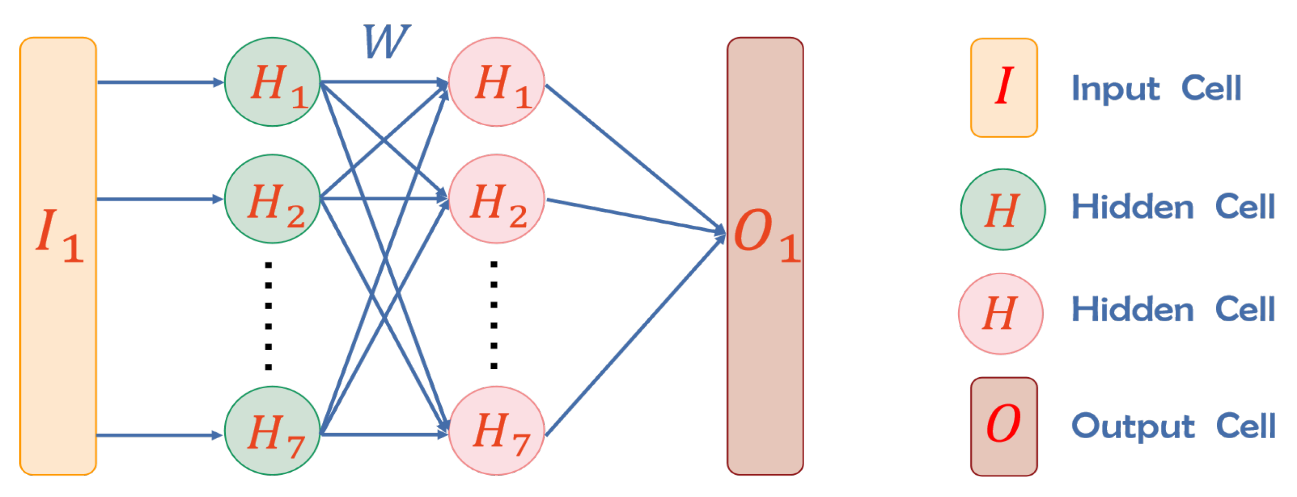
In this work, we construct the following four-layer neural network, which comprises two hidden layers and is equipped with the sigmoid activation function, as exemplified in Figure 1.

Figure 1.
Schematic diagram of neural network operation.
Then, according to Lemma 2, it is shown that can be approximated to given in (2) by a BP neural network, which is stated as follows.
Proposition 1.
Given , for any , there exists a population flow neural network model such that
for any .
4. Error Analysis for Learning-Informed Population Model
In practical environments, population migration data are constantly changing and contain difficult-to-capture patterns. Through neural network tools and a certain amount of data, this population mobility pattern can be approximately expressed. Due to Proposition 1, the unknown population migration function in (2) can be replaced with the population migration neural network model obtained in the last section to obtain the following approximate system:
Since the Sigmoid functions given in (11) are Lipschitz continuous on , then trained by a BP neural network is also Lipschitz continuous. Following the strategy adopted in Theorem 1, it can be seen that (16) also admits a unique solution, given as follows.
Corollary 1.
For any given initial value and any , system (2) admits a unique solution:
Remark 2.
Through the properties of Sigmoid functions, it is easy to observe that the trained population transfer function has good regularity. From Corollary 1, the neural network training function can be used to analyze the characteristics and patterns of population migration.
Theorem 2.
Proof.
For given , assume and are the solutions of (2) and (16), respectively, defined on . Subtract system (2) from system (16) to obtain
where is defined on . Multiplying the first equation of (19) by and integrating on the interval gives
By considering the boundary conditions of (19) and performing integration by parts, we have
Then, putting (21) into (20) leads to
Since satisfies the global Lipschitz condition (5), the above inequality becomes
Due to and , by Hölder’s inequality, one has
Substituting the above inequality into (23) and utilizing Young’s inequality (), one has
with Young’s parameter . Then, Gronwall’s inequality is applied to deduce
In light of Proposition 1, we can conclude that
for any . Then, setting , for any , one can derive from (26) that
Inserting into the above inequality leads to
which implies that in the space . This completes the proof of the theorem. □
Remark 3.
According to Theorem 2, it is easy to find that the population migration neural network model (16) can replace model (2) for population prediction.
5. Numerical Simulation
In this section, a series of simulation experiments will be presented to illustrate the effectiveness of the learning-informed population model in simulating the changing behavior of population migration. For this, there is a need to discretize the original PDE system (2) by using the finite difference method. We set the initial data , the maximum human lifespan , and the final time . Moreover, we let points to build the uniform discretization intervals and , respectively; that is, we establish the following uniform grid on , i.e.,
with the age step and time step . Then, the solution to (2) can be approximated as , where i and j represent discrete time and age variables, respectively. Thus, system (2) can be rewritten as a completely implicit numerical scheme as follows:
where D represents the central difference operator defined by . In our simulation examples, we assume that the mortality rate for any and ; the total productivity of women of childbearing age ; the proportion of females in the population function ; the fertility pattern ; and the reproductive age .
To obtain the learning-informed discrete system corresponding to (31), we first generate the training data pairs , where comes from the solution of system (31), with borrowed from biological models [31], and can be formulated as
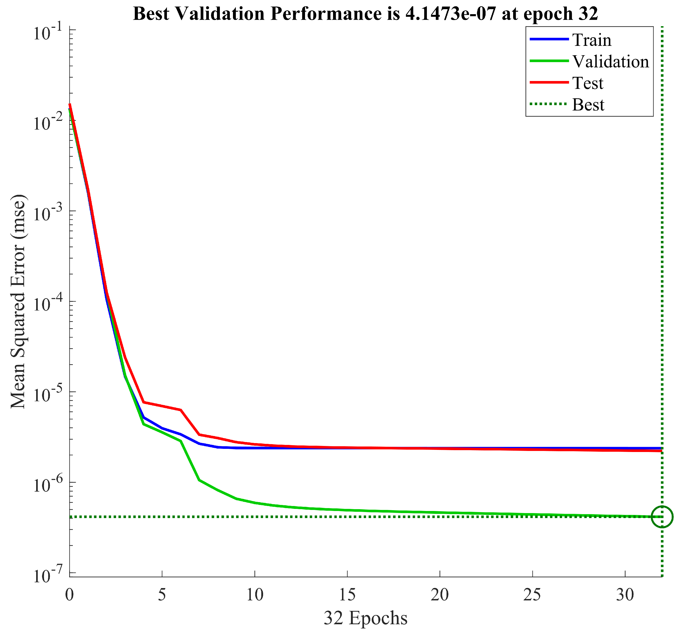
by the first equation of (31). Then, the population migration function can be trained with the BP neural network. Figure 2 illustrates the time evolution of the Mean Square Error (MSE) of a neural network with respect to the round during the training, validation, and testing phases. It is clear that the error of the neural network gradually decreases and eventually plateaus. Moreover, the neural network achieves the best verification performance, , in the 32nd round.
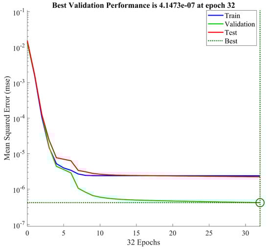
Figure 2.
Neural network fitting error plot.
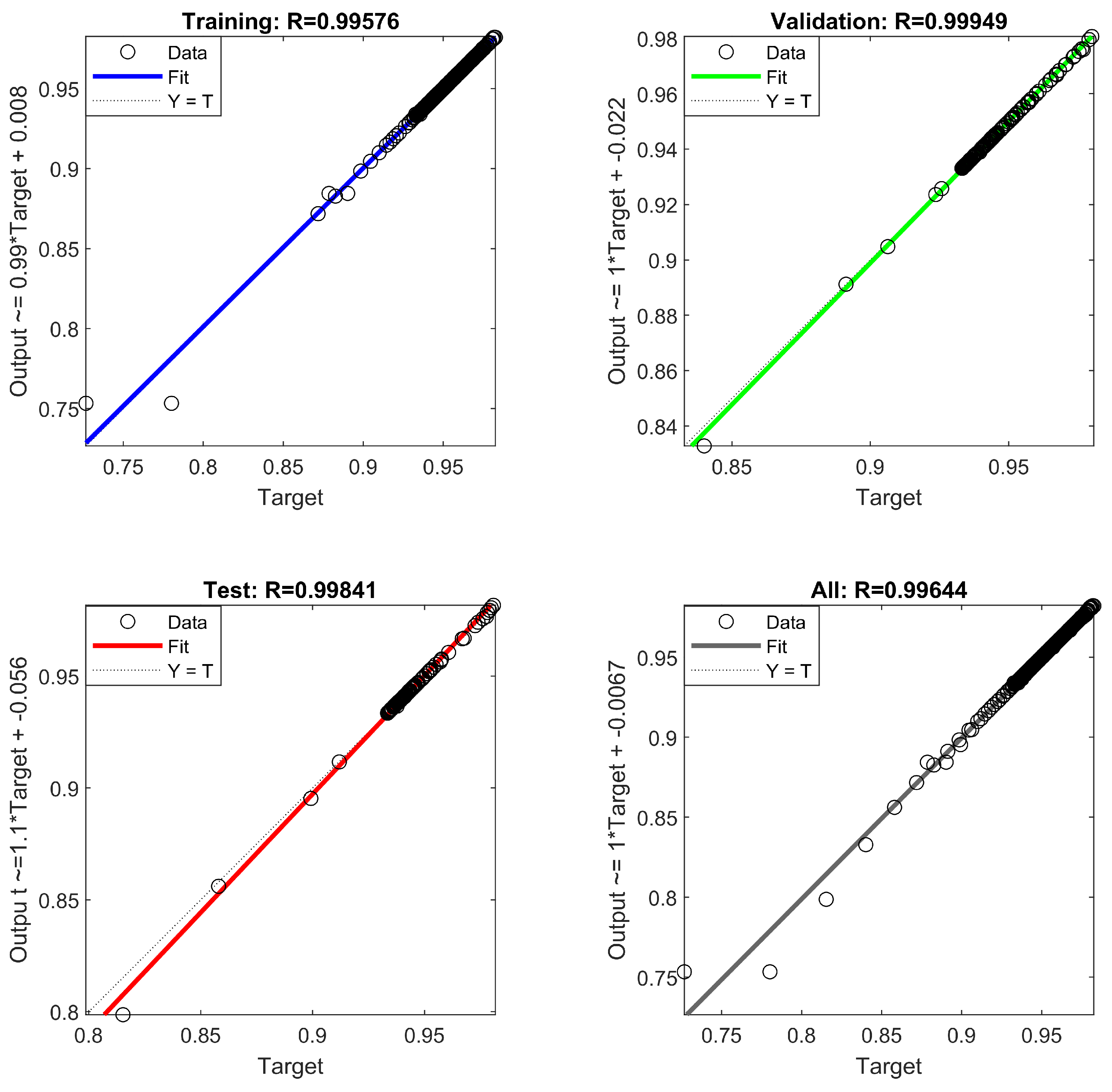
In addition, we observe in Figure 3 that the R-square (coefficient of determination) of the neural network in the training, validation, and testing stages has reached more than 0.99, which indicates the accuracy and effectiveness of the neural network.
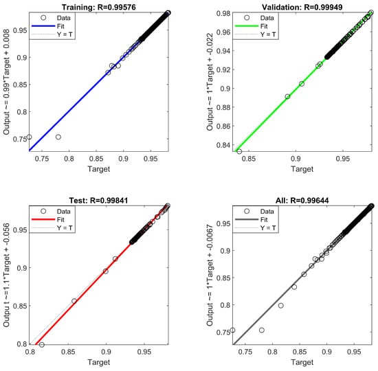
Figure 3.
Coefficient of determination.
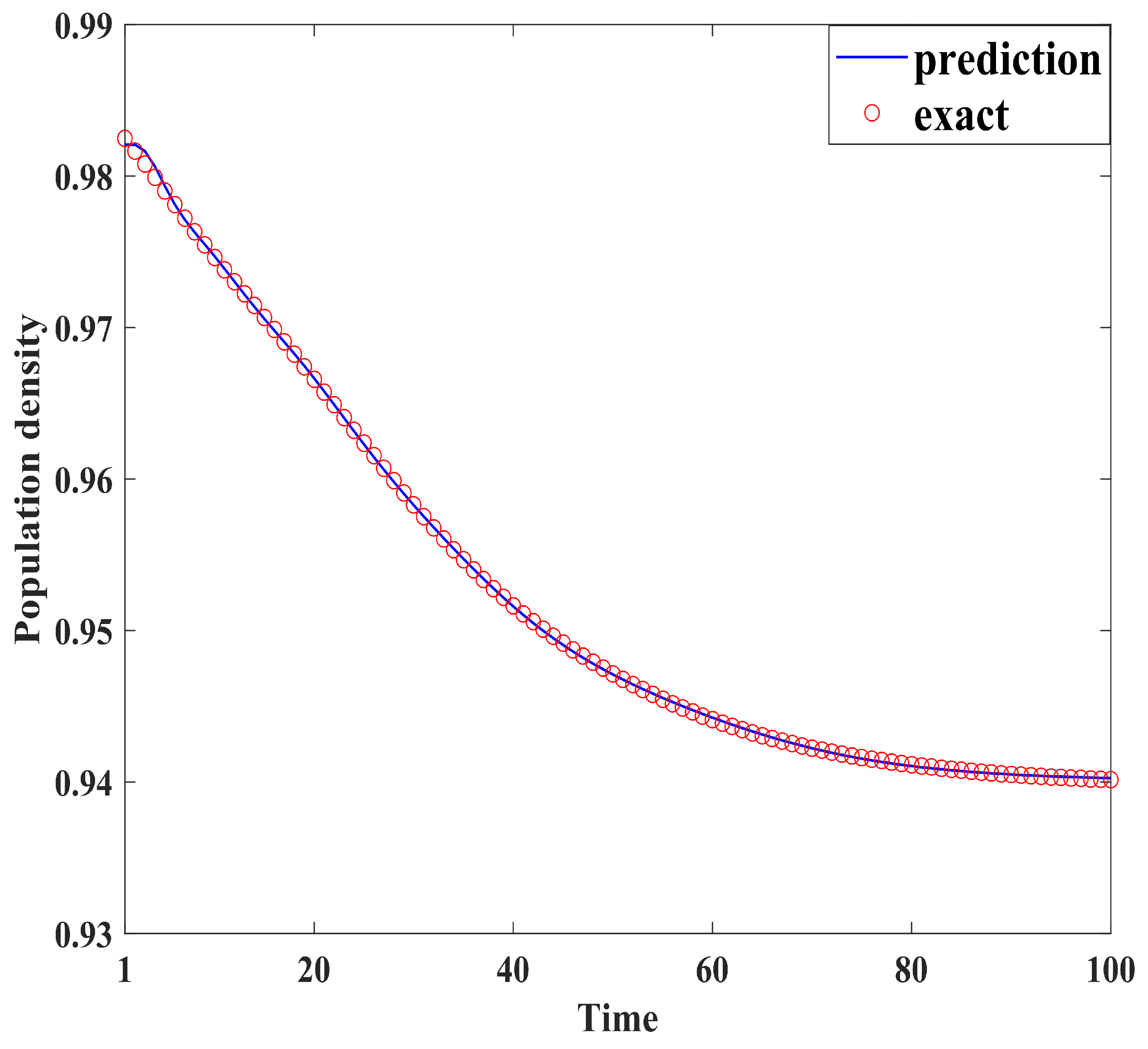
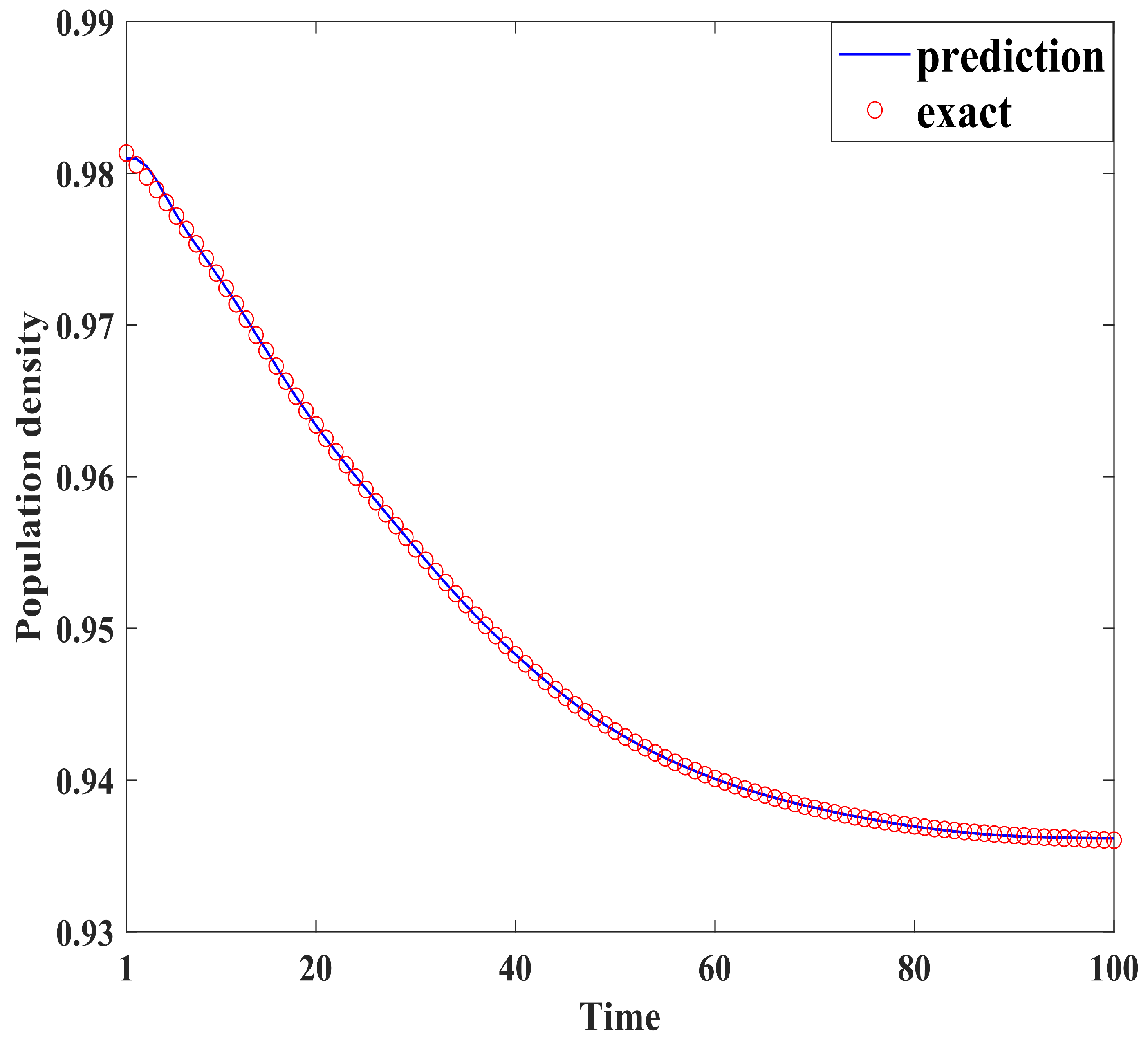
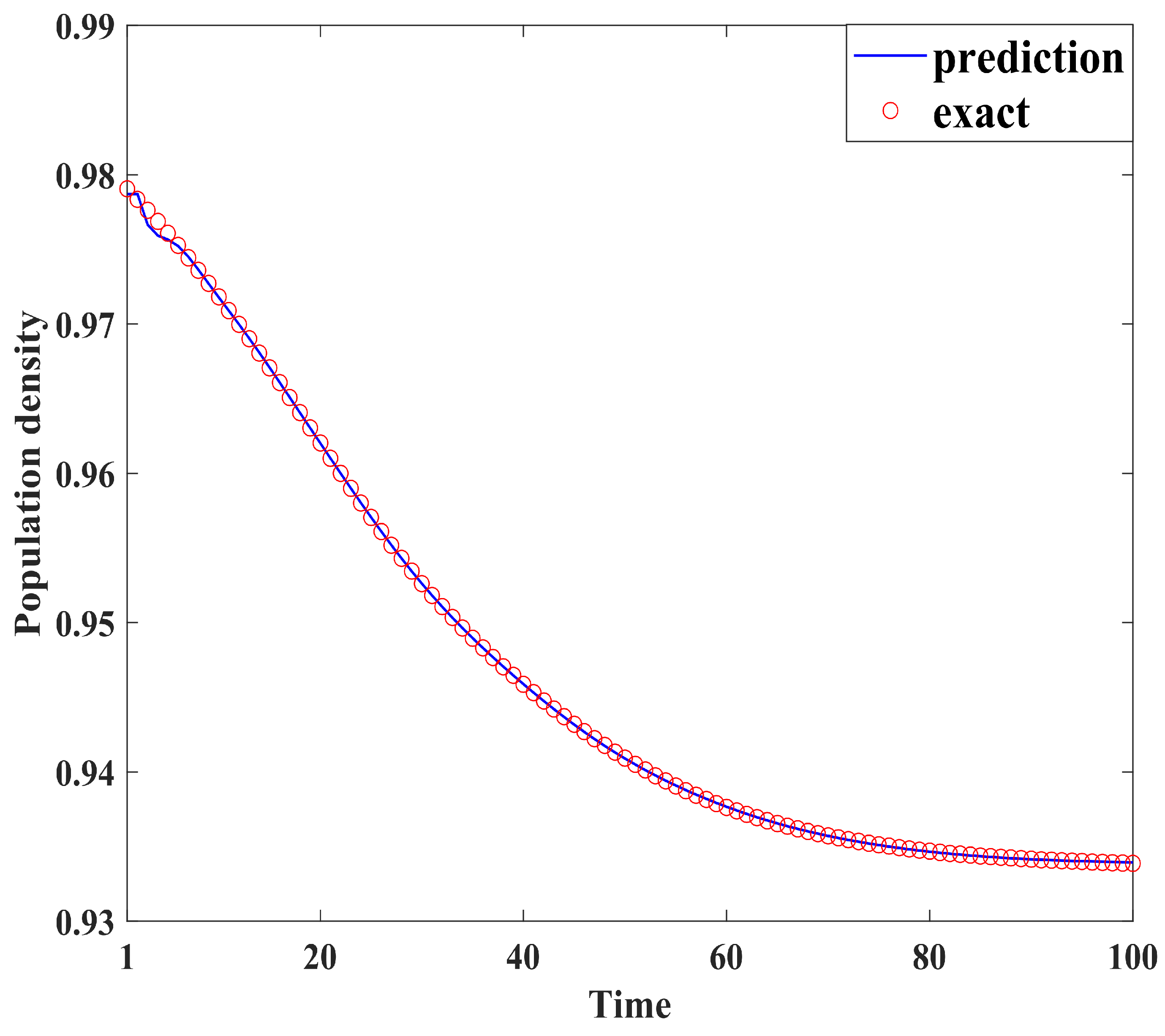
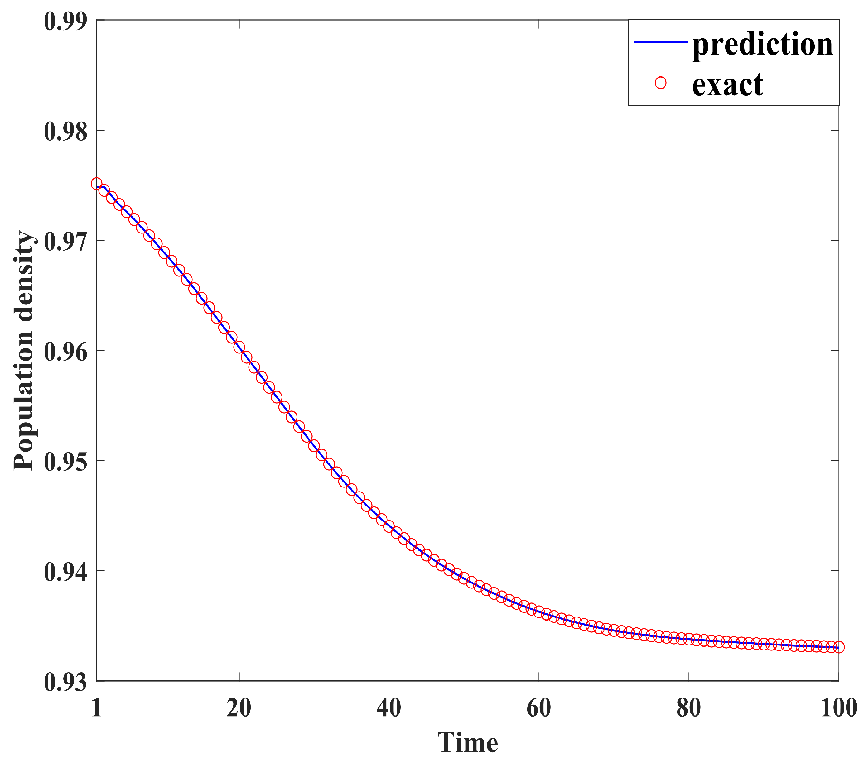
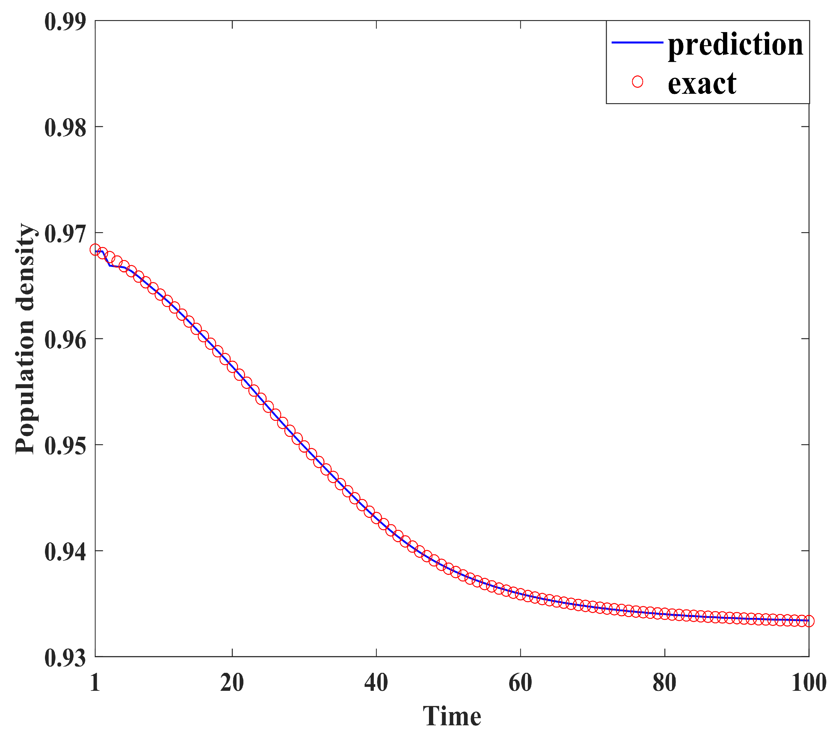
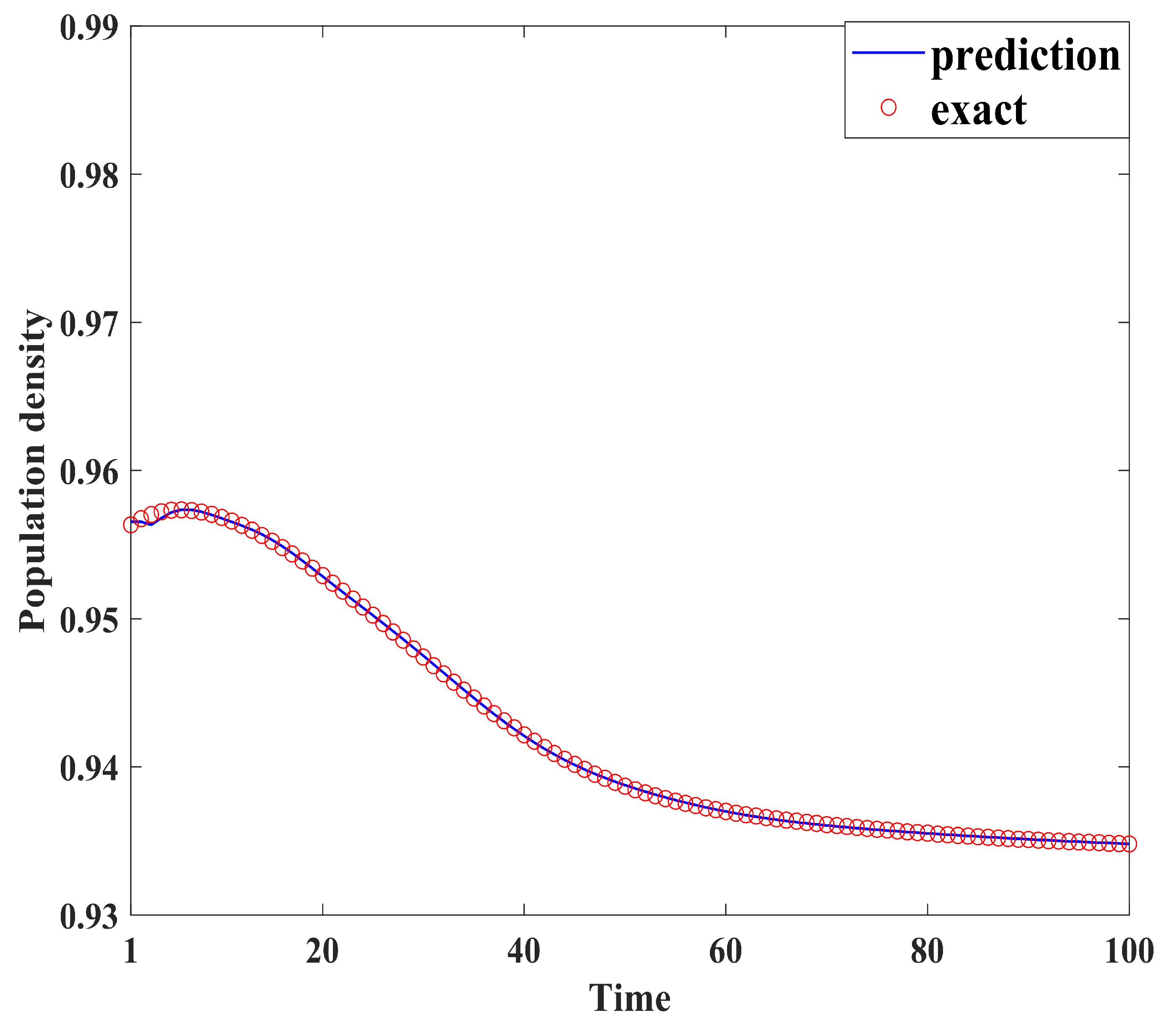
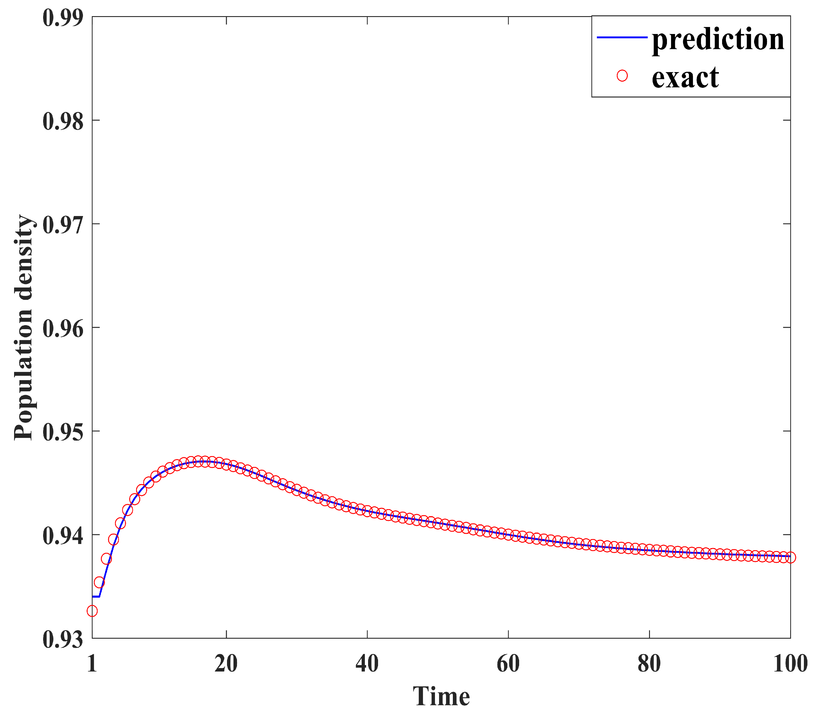
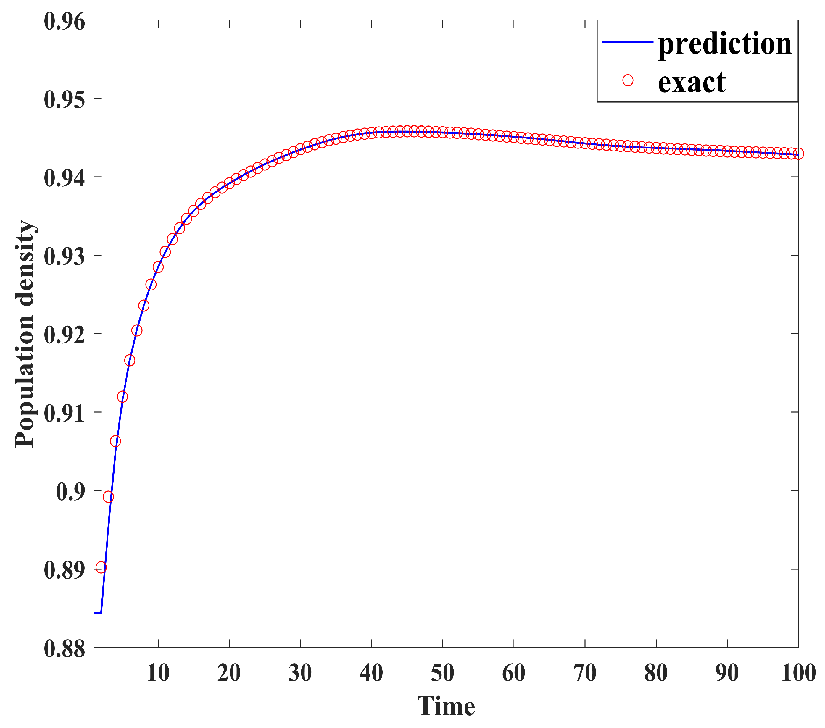
Figure 4, Figure 5, Figure 6, Figure 7, Figure 8, Figure 9, Figure 10 and Figure 11 demonstrate the effectiveness of neural network fitting for the population flow function, including ages 10, 20, 30, 40, 50, 60, 70, and 80. It is shown that the predictions made by the neural network model fit well with the actual data , which is consistent with the theorem in Section 4.
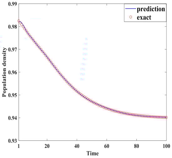
Figure 4.
Ten years old.
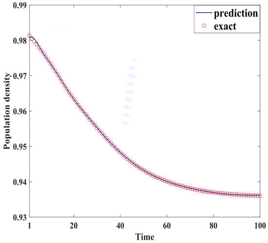
Figure 5.
Twenty years old.

Figure 6.
Thirty years old.
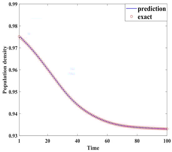
Figure 7.
Forty years old.
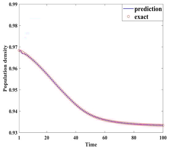
Figure 8.
Fifty years old.
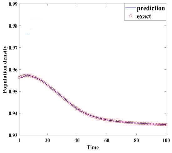
Figure 9.
Sixty years old.
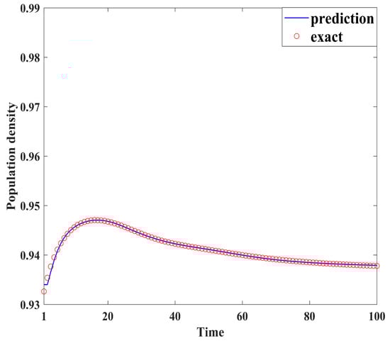
Figure 10.
Seventy years old.
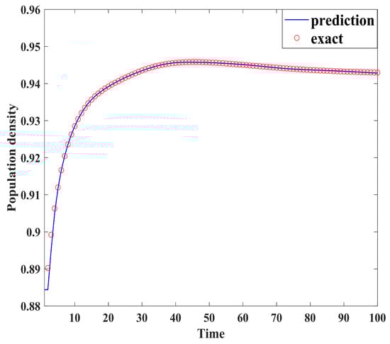
Figure 11.
Eighty years old.
By comparing the results of the neural network fitting with the actual data, the accuracy and effectiveness of the population forecasting model are demonstrated.
6. Conclusions
This article reconstructs a population PDE system with uncertain population migration rates by using neural network methods, where the population migration function has been trained. Firstly, we have established the well-posedness of the learning-informed PDE system by means of semigroup theory. Secondly, we have concluded that the solution of the learning-informed system converges to that of the original system in the sense of . Finally, simulation experiments are provided to verify the effectiveness of the learning-informed system in predicting the proposed population migration changes. Applying this neural network model can help us understand the laws of population dynamics, predict their development trends, and provide a scientific basis for formulating reasonable social policies, optimizing resource allocation, promoting economic development, ensuring social welfare, and achieving sustainable development. How to predict birth and death rates within a population based on existing data using neural network methods remains an open question, which is the focus of our future work.
Author Contributions
Writing—review and editing, C.L.; writing—original draft preparation, Y.W.; formal analysis, Y.C.; formal analysis, Y.G.; investigation, K.W.; funding acquisition, J.Z. All authors have read and agreed to the published version of the manuscript.
Funding
This research was supported by the National Defense Science and Technology Innovation Research Center Project of the PLA Academy of Military Sciences: Data Collection and Modeling Research on Regional Population Migration and Growth, and Science and Technology Project of Liaoning Provincial Department of Education under Grant LJ212410167056.
Data Availability Statement
The data are available from the corresponding author on reasonable request.
Conflicts of Interest
The authors declare no conflicts of interest.
References
- Bloom, D.E.; Boersch-Supan, A.; McGee, P.; Seike, A. Population aging: Facts, challenges, and responses. Benefits Compens. Int. 2011, 41, 22. [Google Scholar]
- Pham, T.N.; Vo, D.H. Aging population and economic growth in developing countries: A quantile regression approach. Emerg. Mark. Financ. Trade 2021, 57, 108–122. [Google Scholar] [CrossRef]
- Supriatna, A.; Susanti, D.; Hertini, E. Application of Holt exponential smoothing and ARIMA method for data population in West Java. In IOP Conference Series: Materials Science and Engineering; IOP Publishing: Bristol, UK, 2017; Volume 166, p. 012034. [Google Scholar] [CrossRef]
- Li, W.; Su, Z.; Guo, P. A prediction model for population change using ARIMA model based on feature extraction. In Journal of Physics: Conference Series; IOP Publishing: Bristol, UK, 2019; Volume 1324, p. 012083. [Google Scholar] [CrossRef]
- Negara, H.R.P. Computational modeling of ARIMA-based G-MFS methods: Long-term forecasting of increasing population. Int. J. Ofemerg. Trends Eng. Res. 2020, 8, 3665–3669. [Google Scholar] [CrossRef]
- Rao, C.; Gao, Y. Influencing factors analysis and development trend prediction of population aging in Wuhan based on TTCCA and MLRA-ARIMA. Soft Comput. 2021, 25, 5533–5557. [Google Scholar] [CrossRef] [PubMed]
- Lanz, B.; Dietz, S.; Swanson, T. Global population growth, technology, and Malthusian constraints: A quantitative growth theoretic perspective. Int. Econ. Rev. 2017, 58, 973–1006. [Google Scholar] [CrossRef]
- Wu, W.Y.; Chen, S.P. A prediction method using the grey model GMC (1, n) combined with the grey relational analysis: A case study on Internet access population forecast. Appl. Math. Comput. 2005, 169, 198–217. [Google Scholar] [CrossRef]
- Tong, M.; Yan, Z.; Chao, L. Research on a grey prediction model of population growth based on a logistic approach. Discret. Dyn. Nat. Soc. 2020, 2020, 2416840. [Google Scholar] [CrossRef]
- Guo, X.; Zhang, R.; Xie, N.; Jin, J. Predicting the Population Growth and Structure of China Based on Grey Fractional-Order Models. J. Math. 2021, 2021, 7725125. [Google Scholar] [CrossRef]
- Zhang, J.; Liu, C.; Jia, Z.; Zhang, X.; Song, Y. The application of a novel grey model in the prediction of China’s aging population. Soft Comput. 2023, 27, 12501–12516. [Google Scholar] [CrossRef]
- Li, Y.; Chen, Y.; Wang, Y. Grey forecasting the impact of population and GDP on the carbon emission in a Chinese region. J. Clean. Prod. 2023, 425, 139025. [Google Scholar] [CrossRef]
- Kong, J.S.D.; Yu, J.Y. Population System Control. Math. Comput. Model. 1988, 11, 11–16. [Google Scholar] [CrossRef]
- Guo, B.Z.; Chan, W.L. A semigroup approach to age-dependent population dynamics with time delay. Commun. Partial. Differ. Equ. 1989, 14, 809–832. [Google Scholar] [CrossRef]
- Guo, B.Z. A finite difference scheme for the equations of population dynamics. Math. Comput. Model. 1995, 21, 75–87. [Google Scholar] [CrossRef]
- Guo, B.Z.; Yao, C.Z. New results on the exponential stability of non-stationary population dynamics. Acta Math. Sci. 1996, 16, 330–337. [Google Scholar] [CrossRef]
- Ainseba, B.; Anita, S. Local exact controllability of the age–dependent population dynamics with diffusion. Abstr. Appl. Anal. 2001, 6, 357–368. [Google Scholar] [CrossRef]
- Anita, S. Analysis and Control of Age-Dependent Population Dynamics; Springer Science & Business Media: Berlin/Heidelberg, Germany, 2013. [Google Scholar] [CrossRef]
- Fragnelli, G.; Yamamoto, M. Carleman estimates and controllability for a degenerate structured population model. Appl. Math. Optim. 2021, 84, 999–1044. [Google Scholar] [CrossRef]
- Hegoburu, N.; Magal, P.; Tucsnak, M. Controllability with positivity constraints of the lotka-mckendrick system. SIAM J. Control Optim. 2018, 56, 723–750. [Google Scholar] [CrossRef]
- Maity, D.; Tucsnak, M.; Zuazua, E. Controllability and positivity constraints in population dynamics with age structuring and diffusion. J. Math. Pures Appl. 2019, 129, 153–179. [Google Scholar] [CrossRef]
- Niaki, S.T.A.; Hoseinzade, S. Forecasting S & P 500 index using artificial neural networks and design of experiments. J. Ind. Eng. Int. 2013, 9, 1. [Google Scholar] [CrossRef]
- Chon, T.S.; Park, Y.S.; Kim, J.M.; Lee, B.Y.; Chung, Y.J.; Kim, Y. Use of an artificial neural network to predict population dynamics of the Forest–Pest pine needle gall midge (Diptera: Cecidomyiida). Environ. Entomol. 2000, 29, 1208–1215. [Google Scholar] [CrossRef]
- Claveria, O.; Monte, E.; Torra, S. Multiple-Input Multiple-Output vs. Single-Input Single-Output Neural Network Forecasting; No. 2015-02; Research Institute of Applied Economics: Barcelona, Spain, 2015. [Google Scholar] [CrossRef]
- Folorunso, O.; Akinwale, A.T.; Asiribo, O.E.; Adeyemo, T.A. Population prediction using artificial neural network. Afr. J. Math. Comput. Sci. Res. 2010, 3, 155–162. [Google Scholar]
- Nordbotten, S. Neural network imputation applied to the Norwegian 1990 population census data. J. Off. Stat. 1996, 12, 385–402. [Google Scholar]
- Tang, Z.; Leung, C.W.; Bagchi, K. Improving population estimation with neural network models. In International Symposium on Neural Networks; Springer: Berlin/Heidelberg, Germany, 2006; pp. 1181–1186. [Google Scholar] [CrossRef]
- Pazy, A. Semigroups of Linear Operators and Applications to Partial Differential Equations; Springer Science and Business Media: Berlin/Heidelberg, Germany, 1983. [Google Scholar] [CrossRef]
- Song, J.; Yu, J.Y. Population Control System; Springer: New York, NY, USA, 1987. [Google Scholar] [CrossRef]
- Dong, G.; Hintermüller, M.; Papafitsoros, K. Optimization with learning-informed differential equation constraints and its applications. ESAIM Control Optim. Calc. Var. 2022, 28, 3. [Google Scholar] [CrossRef]
- Ma, L.; Wang, H.; Gao, J. Dynamics of two-species Holling type-II predator-prey system with cross-diffusion. J. Differ. Equ. 2023, 365, 591–635. [Google Scholar] [CrossRef]
Disclaimer/Publisher’s Note: The statements, opinions and data contained in all publications are solely those of the individual author(s) and contributor(s) and not of MDPI and/or the editor(s). MDPI and/or the editor(s) disclaim responsibility for any injury to people or property resulting from any ideas, methods, instructions or products referred to in the content. |
© 2025 by the authors. Licensee MDPI, Basel, Switzerland. This article is an open access article distributed under the terms and conditions of the Creative Commons Attribution (CC BY) license (https://creativecommons.org/licenses/by/4.0/).