A Wide-Range Adjustable Conservative Memristive Hyperchaotic System with Transient Quasi-Periodic Characteristics and Encryption Application

Abstract

In comparison with dissipative chaos, conservative chaos is better equipped to handle the risks associated with the reconstruction of phase space due to the absence of attractors. This paper proposes a novel five-dimensional (5D) conservative memristive hyperchaotic system (CMHS), by incorporating memristors into a four-dimensional (4D) conservative chaotic system (CCS). We conducted a comprehensive analysis, using Lyapunov exponent diagrams, bifurcation diagrams, phase portraits, equilibrium points, and spectral entropy maps to thoroughly verify the system’s chaotic and conservative properties. The system exhibited characteristics such as hyperchaos and multi-stability over an ultra-wide range of parameters and initial values, accompanied by transient quasi-periodic phenomena. Subsequently, the pseudorandom sequences generated by the new system were tested and demonstrated excellent performance, passing all the tests set by the National Institute of Standards and Technology (NIST). In the final stage of the research, an image-encryption application based on the 5D CMHS was proposed. Through security analysis, the feasibility and security of the image-encryption algorithm were confirmed.

1. Introduction

In recent years, chaotic systems have become crucial in fields like image encryption [1,2,3], neural networks [4,5,6], secure communications [7,8,9], and the generation of pseudo-random numbers [10,11,12]. This is largely due to their extreme sensitivity to initial conditions and parameters, coupled with their inherent unpredictability [13,14,15]. Given that a multitude of natural phenomena can be represented by dissipative chaotic systems (DCSs), numerous such systems have been introduced by researchers over the years. Notable examples include the Chen system [16], the Chua system [17], the Lu system [18], the Sprott system [19], and the Lorenz system [20]. However, the study of conservative chaotic systems (CCSs) remains less explored. Unlike their dissipative counterparts, CCSs typically lack the concept of attractors [21]. They are characterized by pseudo-randomness and exhibit properties akin to white noise. These features suggest that CCSs hold significant potential for broader applications, particularly in the realm of information encryption.

Due to the many advantages that CCSs possess that DCSs lack, numerous scholars have shifted their focus to the realm of conservative chaos [22,23]. They have proposed a multitude of methods for constructing CCSs. These have led to the emergence of many new CCSs with complex dynamics, filling significant gaps in the field. One such approach is the use of fractional-order systems to generate conservative chaos. In 2017, Cang et al. [24] introduced two 4D CCSs with conservative flows. In 2021, Leng et al. [25] proposed a 4D fractional-order system with both dissipative and conservative properties, based on the Case A system previously outlined by Cang. This new system demonstrated exceptional stability and transient characteristics. The following year, Leng et al. [26] constructed a novel fractional-order CCS. It was discovered in the paper that by altering the order or parameters of the system, a conservative system could exhibit dissipative phenomena. The system’s hardware implementation was carried out on a DSP experimental platform, confirming the accuracy of the theoretical analysis. Tian et al. [27] proposed a novel 5D conservative hyperchaotic system, utilizing the Adomian decomposition method (ADM) [28,29] to transform an integer-order system into a fractional-order system.

Another method for constructing CCSs involves the application of Euler’s equations, which describe three-dimensional (3D) rigid bodies [30]. This technique couples low-dimensional rigid body sub-equations by introducing a Hamiltonian vector field to obtain high-dimensional generalized Euler equations. However, both the Hamiltonian and Casimir energy conservation of the resulting equations are preserved. To induce chaos, this method typically disrupts the conservation of Casimir energy by introducing constants while maintaining the conservation of Hamiltonian energy, at which point chaos arises. Numerous articles have constructed Hamiltonian CCSs by using this method [31]. Qi et al. [32] proposed a 4D CCS with co-existing chaotic orbits by breaking the conservation of Casimir energy. Based on the rigid body Euler equation of binary product, Pan et al. [33] proposed an effective method to construct high-dimensional CCSs based on skew-symmetric matrices and designed the 4D, 5D, and 6D Hamiltonian CCSs. It was proved mathematically that the system constructed by this method satisfies the conservation of Casimir energy and Hamiltonian energy.

Additionally, there is a method for constructing CCSs based on the special structure of cyclic symmetric systems [34] that has garnered much attention from scholars, due to the property that all state equations share the same structure [35]. Among those scholars, Zhang has made significant contributions in this area. Zhang et al. [36] proposed a new method for constructing cyclic symmetric conservative chaos, which is applicable to the construction of 3D and higher-dimensional systems. In their paper, not only were the chaotic properties of the constructed systems determined by scattering, equilibrium points, and Lyapunov exponents, but also Zhang improved the offset-enhanced control of three CCSs constructed by him, and the system was ultimately implemented using a DSP hardware platform. In 2024, Zhang et al. [37] used a 4D system and a 5D system as examples. The 4D system exhibited extreme multiple stability of homogeneity and heterogeneity with the introduction of a sinusoidal function term. The 5D system improved the offset enhancement control by using the introduction of the absolute value, thus exhibiting extreme multiple stability in multiple directions and achieving hyperchaotic roaming. Ultimately, in their paper, the 5D system was used as an example of the application of the circular symmetric conservative system in data-encrypted transmission. However, most of the aforementioned studies proposed low-dimensional chaotic systems with a relatively narrow window for system control parameters. In practical applications, if the system parameters could vary over a wide range while the system remained chaotic then this would be highly advantageous in areas such as secure communication and chaos control [38,39].

To obtain chaotic systems with a broad parameter range, it is often necessary to introduce nonlinear terms or extend the system to higher dimensions. In 2022, Zhang et al. [40] proposed a 5D Hamiltonian conserved hyperchaotic system with equilibrium points of four center types, a wide parameter range, and co-existing hyperchaotic orbits. In 2024, Huang et al. [41] proposed a 5D symmetric Hamiltonian system with hidden multiple stability. In 2023, Wu et al. [42] proposed a modeling method for a class of 7D CCSs based on previous studies, which can maintain stable chaotic properties under a wide range of parameter variations. In the same year, Zhang et al. [43] constructed a 5D conservative hyperchaotic system by deriving four 5D sub-Euler equations and combining them with existing sub-Euler equations to obtain ten 5D sub-Euler equations, which have a wide range of initial values and are multiply stable; and Zhou et al. [44] proposed a new n-dimensional conservative chaotic model in 2023: this system has an extensive parameter range and possesses a high maximum Lyapunov exponent. Ultimately, the authors applied this system to the field of image encryption.

In this paper, by incorporating a memristor into a 4D CCS, a 5D CMHS is constructed. This system exhibits a rich array of phenomena, such as hyperchaos and transient quasi-periodicity across a broad spectrum of parameters and initial values. The principal contributions of this paper are as follows:

(1) A new 5D CMHS is proposed, and its conservation is demonstrated through the analysis of divergence and the Kaplan–Yorke dimension.

(2) The dynamics of the 5D CMHS are analyzed from multiple perspectives. The analyses indicate that the proposed system remains hyperchaotic over a wide range of parameters, characterized by an infinite number of equilibrium points and transient quasi-periodicity.

(3) The system’s chaotic sequence is tested by NIST, and the outcomes show that the sequence passes all 15 NIST tests, signifying that the system possesses hyperchaotic properties suitable for a pseudo-random number generator.

(4) Based on the proposed 5D CMHS, an image-encryption algorithm is presented. From a security perspective, its feasibility is demonstrated, and its superiority is proven by comparison with other encryption algorithms.

In Section 2, the construction of a 5D CMHS is presented, along with proof of its conservativity. In Section 3, the fundamental dynamical behaviors of the system are analyzed. Section 4 investigates the hyperchaotic behavior and transient quasi-periodicity of the system over a broad range of parameters. In Section 5 and Section 6, the 5D CMHS is tested by NIST and its application to image encryption based on the newly proposed 5D CMHS is explored. Section 7 summarizes the work presented in this paper.

2. Modeling of 5D CMHS

2.1. Introduction to Memristors

As a resistor with memory, a memristor’s resistance is determined not only by the current voltage and current but also by the amount of charge that has previously passed through it [45,46]. This characteristic endows memristors with unique advantages in constructing CCSs. The nonlinear properties of memristors can significantly enhance the dynamic behavior of a system, enabling it to exhibit more complex chaotic characteristics, such as multiscroll, hyperchaos, and extreme multistability. Moreover, the introduction of memristors makes the system more sensitive to initial conditions, thereby enhancing the security performance of image-encryption algorithms based on memristor-chaotic systems.

The central concept of the present paper is to incorporate a memristor into a 4D CCS, to examine and dissect the characteristics of the emergent system. The description of the referenced memristor model is as follows:

$$\left\{\begin{array}{c}i=W\left(\phi \right)v=\left(k{u}^2+b\right)v\hfill \\ {\displaystyle \frac{d\phi }{dt}}=v\hfill \end{array}\right.$$

(1)

where v and i are the output voltage and input current, respectively. W is a continuous function of $\phi$ and is called memductance. In [24], two new CCSs were proposed as the Case A and Case B systems, where the Case A system was a Hamiltonian energy-conserving and volume-conserving bi-conservative 4D CCS with complex dynamical properties. Its system model is shown in Equation (2):

$$\left\{\begin{array}{c}\dot{x}=ayw\hfill \\ \dot{y}=xz\hfill \\ \dot{z}=-xy+bw\hfill \\ \dot{w}=-axy-bz\hfill \end{array}\right.$$

(2)

where $x,y,z$, and w are the system state variables, a and b are the system parameters, and for certain parameter values the LEs sum to zero and the system has rich dynamics, which is manifested by the transformation of the system from a chaotic state to a quasi-periodic state as parameter b is varied.

In the study of system (2), we select the system variable as the control voltage of the memristor, to introduce the whole memristor output W ($\phi$) into the system as a negative feedback control, and we obtain a new 5D CMHS. The mathematical model of the new system can be described as follows:

$$\left\{\begin{array}{c}\dot{x}=ayw\hfill \\ \dot{y}=xz(k{u}^2+b)\hfill \\ \dot{z}=-xy+bw\hfill \\ \dot{w}=-axy-bz\hfill \\ \dot{u}=x\hfill \end{array}\right.$$

(3)

where $x,y,z,w,u$ are system state variables and $a,b,k$ are system parameters. The parameters are chosen as $(a,b,k)$ = (10, 5, 2) and the initial values are chosen as $(x,y,z,w,u)$ = (1, 1, 1, 1, 1). With the introduction of the memristor, we will not subsequently consider its physical meaning in this paper, but only its mathematical meaning, and we will analyze it as a part of the system as a whole. Next, we analyze system (3), in terms of conservativeness and dynamics.

2.2. Conservative Analysis

2.2.1. Divergence Analysis

Chaotic systems are mainly divided into DCSs and CCSs. The divergence ∇·F is mainly relied on to distinguish these two systems: the system is a DCS when the system divergence ∇·F < 0, and it is a CCS when ∇·F = 0. For system (3), the divergence is

$$\nabla ·F={\displaystyle \frac{d\dot{x}}{dx}}+{\displaystyle \frac{d\dot{y}}{dy}}+{\displaystyle \frac{d\dot{z}}{dz}}+{\displaystyle \frac{d\dot{w}}{dw}}+{\displaystyle \frac{d\dot{u}}{du}}=0$$

(4)

It can be seen that the system ∇·F = 0, indicating that the system is volume-conservative.

2.2.2. Kaplan–Yorke Dimensional Analysis

In 1963, Kaplan–Yorke proposed the Lyapunov dimension to determine the type of attractor in dynamical systems and that the dimension of the singular attractor must be lower than the spatial dimension of the dynamical system; then, CCSs lack singular attractors, so the Lyapunov dimension must be equal to the dimension of the dynamical system. The Kaplan–Yorke dimension of system (3) is calculated as follows:

$$D_L=4+{\displaystyle \frac{L{E}_1+L{E}_2+L{E}_3+L{E}_4}{\left|L{E}_5\right|}}=5$$

(5)

The Kaplan–Yorke dimension of system (3) is not only an integer but is also equal to the dimension of the system, which again proves that system (3) is a CCS.

3. Basic Dynamics Analysis

3.1. Lyapunov Exponents

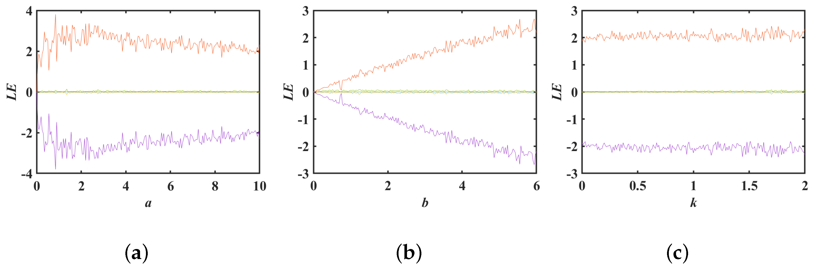
In general, a nonlinear system is classified as chaotic if it has at least one positive LE and hyperchaotic if there are two or more positive LEs [47,48]. A chaotic system is termed a DCS if the sum of its LEs is negative and a CCS if the sum is zero. To investigate the impact of parameter variations on the system’s behavior, we altered one system parameter while keeping the other two fixed. We then derived the Lyapunov exponential maps for system (3) with respect to the parameters a, b, and k, as illustrated in Figure 1.

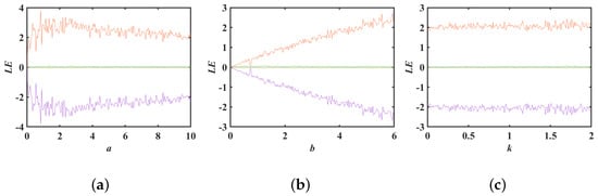
Figure 1. Lyapunov exponents for system (3): (a) $a\in [0,10]$; (b) $b\in [0,6]$; (c) $k\in [0,2]$.

From Figure 1, it is evident that the LEs of system (3) were symmetrically distributed around 0 as the system parameters changed. There were two LEs that were notably greater than 0, signifying that system (3) is a 5D hyperchaotic conservative system. As depicted in Figure 1a, the first Lyapunov exponent decreased initially and then stabilized with the variation of parameter a. Similar to parameter a, the first Lyapunov exponent in Figure 1c fluctuated with parameter k and hovered around $LE=2$ for $k\in (0,2)$. Parameter b exhibited a more intriguing behavior; the maximum Lyapunov exponent of the system increased almost linearly with the increment of parameter b, as shown in Figure 1b. This phenomenon will be analyzed in greater detail in subsequent sections.

3.2. Bifurcation Diagram

The bifurcation diagram is a tool for analyzing the bifurcation phenomenon of a system when the parameters are changing, and it can show more intuitively the evolution of the system from a periodic state to a chaotic state under the change of parameters. By analyzing the bifurcation diagram, the complex behavior of the system can be understood in depth.

The bifurcation diagram of system (3) for each parameter variation is shown in Figure 2. Unlike the DCS, in these three bifurcation diagrams it can be clearly seen that system (3) immediately entered into a hyperchaotic state. This was because the CCS had no attractor, so the initial state of the system was in the hyperchaotic region. The bifurcation maps shown in Figure 2 have a more uniform density of points as well as coverage, which corresponds with the results of the Lyapunov exponential maps in Figure 1:

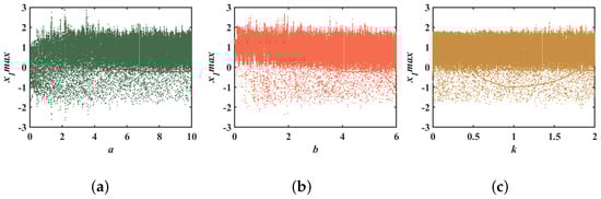
Figure 2. Bifurcation diagram for system (3): (a) $a\in [0,10]$; (b) $b\in [0,6]$; (c) $k\in [0,2]$.

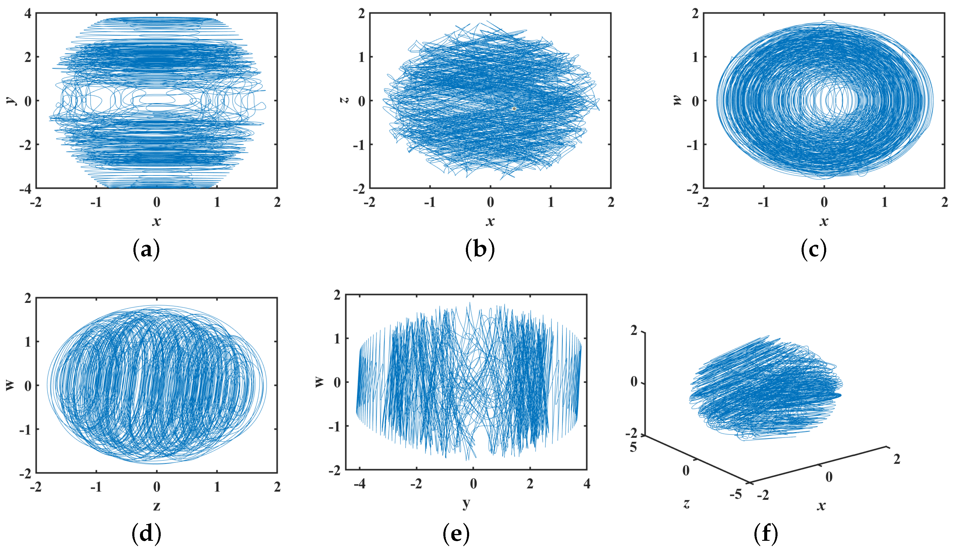
3.3. Phase Diagram

A phase diagram is an image of a system’s trajectory in phase space over time for a finite period of time, where each point on the trajectory represents a state of the system in phase space and the evolutionary trajectory consists of these points. The phase diagram can visualize the trajectories, boundaries, and chaotic attractors of a chaotic system. In the case of CCSs, where the phase volume is conserved and, therefore, does not shrink as the evolution progresses, no obvious attractors can be observed in the phase diagram.

Although CCSs do not have obvious attractors, they can be used to visualize the trajectory of the system and to analyze the dynamical behavior of the system. Therefore, it is still necessary to observe the phase diagram of the system when studying CCSs. The phase diagram of system (3) is shown in Figure 3. From the figure, it can be seen that the phase trajectories are spread over the whole phase space and there are no attractors, which again proves that system (3) is a CCS:

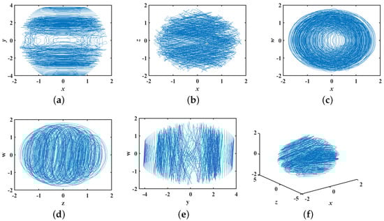
Figure 3. Phase diagram: (a) $x-y$; (b) $x-z$; (c) $x-w$; (d) $z-w$; (e) $y-w$; (f) $x-y-z$.

3.4. Equilibrium Analysis

Equilibrium points are typically utilized to analyze the stability of nonlinear systems. However, CCSs, unlike their dissipative counterparts, do not possess attractors, in the general sense. CCSs with constant phase volume are incapable of gradually converging to an equilibrium point. As such, these systems feature only a center point and a saddle point [49]. To identify the equilibrium point of system (3), equate the left-hand side of each equation to zero:

$$\left\{\begin{array}{c}0=ayw\hfill \\ 0=xz(k{u}^2+b)\hfill \\ 0=-xy+bw\hfill \\ 0=-axy-bz\hfill \\ 0=x\hfill \end{array}\right.$$

(6)

From the fifth equation, it can be seen that x is equal to 0. Substituting x is equal to 0 into the third and fourth equations, respectively, since $a,b$, and k are all positive, it can be obtained that z and w are equal to 0. Therefore, y and u are free and can be taken as any constants to establish the equilibrium points as (0, $l_2$, 0, 0, 0, $l_5$).

The equilibrium points of the system are obtained as (0, 0, 0, 0, 0), (0, 0, 0, 0, $l_5$), (0, $l_2$, 0, 0, 0), and (0, $l_2$, 0, 0, $l_5$), including the origin and the line plane. Substitute the equilibrium points into the Jacobi matrix of the system:

$$J=\left[\begin{array}{ccccc}0& a{w}_{*}& 0& a{y}_{*}& 0\\ z_{*}(k{u}_{*}^2+b)& 0& x_{*}(k{u}_{*}^2+b)& 0& 2k{x}_{*}{z}_{*}{u}_{*}\\ -y_{*}& -x_{*}& 0& b& 0\\ -a{y}_{*}& -a{x}_{*}& b& 0& 0\\ 1& 0& 0& 0& 0\end{array}\right]$$

(7)

With the characteristic polynomial, the corresponding characteristic polynomial can be obtained:

$$P_1\left(\lambda \right)=P_2\left(\lambda \right)={\lambda }^3({\lambda }^2-b^2)$$

(8)

$$P_3\left(\lambda \right)=P_4\left(\lambda \right)={\lambda }^2({\lambda }^3+ab{l}_2^2+\lambda a^2{l}_2^2-\lambda b^2)$$

(9)

For Equation (9), we can easily obtain that ${\lambda }_1$ and ${\lambda }_2$ are 0, while ${\lambda }_3$, ${\lambda }_4$, and ${\lambda }_5$ must satisfy the following equations:

$$\begin{array}{cc}& (\lambda -{\lambda }_3)(\lambda -{\lambda }_4)(\lambda -{\lambda }_5)\hfill \\ & ={\lambda }^3-{\lambda }^2({\lambda }_2+{\lambda }_3+{\lambda }_4)+\lambda ({\lambda }_3{\lambda }_2+{\lambda }_2{\lambda }_3+{\lambda }_1{\lambda }_3)-{\lambda }_1{\lambda }_2{\lambda }_3\hfill \\ & =0\hfill \end{array}$$

(10)

By comparison, it can be obtained that ${\lambda }_1$+${\lambda }_2$+${\lambda }_3$=0 and ${\lambda }_1$${\lambda }_2$${\lambda }_3$≠0. The parameters a and b are greater than 0, which means that the values ${\lambda }_1$, ${\lambda }_2$, and ${\lambda }_3$ cannot be on one side of the imaginary axis, but can only be distributed on the two sides of the real axis. Therefore, the equilibrium point types of $P_3\left(\lambda \right)$ and $P_4\left(\lambda \right)$ are all saddle points.

We set $(i=1,2,3,4)$ and obtain the corresponding eigenvalues. The eigenvalues and types of equilibrium points are listed in Table 1. The types of equilibrium points for system (3) are all saddle points, and there are no foci or nodes. This is consistent with the nature of the equilibrium points of the conservative system described earlier.

Table 1. The equilibrium point and corresponding types.

Equilibrium Points	Characteristic Values	Type
(${\mathit{l}}_{\mathbf{2}},{\mathit{l}}_{\mathbf{5}}\in \mathit{R}$)	($\mathit{\alpha },\mathit{\beta },\mathit{\gamma }>\mathbf{0}$)
$l_2$=0	(0,0,0,$\pm \alpha$)	Saddle
$l_2$≠0	(0,0,$\alpha$,$\beta$,$-\gamma$)	Saddle
	(0,0,$\alpha$,$-\beta$,$\gamma$)	Saddle
	(0,0,$\alpha$,$-\beta$,$-\gamma$)	Saddle

4. Hyperchaos Under Wide Range

The traditional chaotic system is not favorable for the practical application of chaotic systems in the field of chaos control, due to its highly dependent sensitivity to parameters and initial values, where the parameters can only be varied within a narrow range or else they will be out of the chaotic state [38,39], as shown in Table 2. In contrast, chaotic systems with wide parameter ranges can maintain the chaotic state in a wide range, which means that the system has good stability.

Table 2. Parameter range of traditional chaotic system.

No.	The System Dimension	Parameter Length of Chaotic State	Reference
1	5D	Less than 100	[50]
2	4D	Less than 6	[51]
3	4D	Less than 10	[52]
4	4D	Less than 50	[39]
5	5D	$[0,500]$	This paper

4.1. Hyperchaos Under Wide Initial Values and Multi-Stability

In DCSs, multi-stability is characterized by the co-existence of multiple attractors. In contrast, CCSs do not have attractors, and, thus, multi-stability is reflected in the co-existence of multiple chaotic trajectories [53,54].

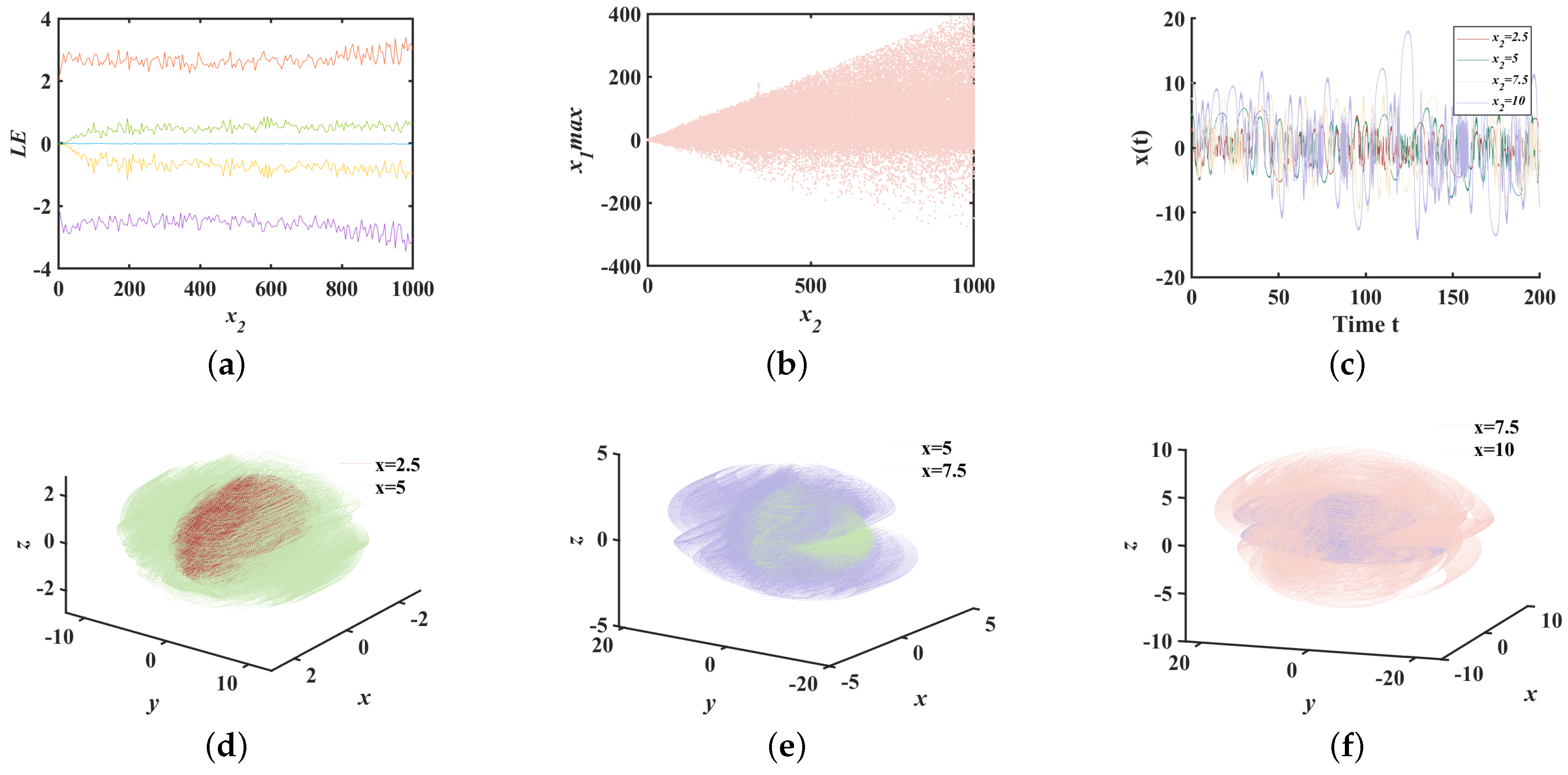
With parameters $(a,b,k)=(10,5,2)$ and initial values $(x_1,x_3,x_4,x_5)=(1,1,1,1)$, the initial value $x_2$ was selected within the interval $(0,1000)$, to plot the Lyapunov exponents and bifurcation diagrams of system (3), as shown in Figure 4a,b. The results indicate that the system consistently resides in the hyperchaotic region, with the maximum Lyapunov exponent stabilizing around 2.3. Notably, within the interval $[0,1000]$, the LEs are symmetric about 0, meaning the sum of the LEs equals 0, which confirms the conservative nature of system (3). It can be clearly seen from Figure 4b that the majority of points are consistently densely distributed, which also indicates that the system is in a state of hyperchaos. Furthermore, as the initial value $x_2$ varies within the range of [0, 1000], the range of points on the y-axis gradually expands. Furthermore, with the initial values of $x_2$ set to 2.5, 5, 7.5, and 10, while keeping the other parameters constant, phase diagrams, and corresponding time series diagrams were obtained, as shown in Figure 4c–f. The co-existence of hyperchaotic trajectories is evident, and it is apparent from the diagrams that different trajectories exhibit varying degrees of ergodicity, which increases with the increase of $x_2$. Figure 4c displays the time series diagrams at corresponding times, showing that as $x_2$ increases, the amplitude of the time-domain waveforms also increases, enhancing the ergodicity and chaotic nature of system (3), which is consistent with the phase diagram analysis.

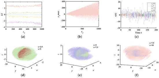
Figure 4. System (3): (a) LEs; (b) bifurcation diagram of $x_2\in [0,1000]$; (c) time series diagram; (d–f) phase gram of $x_2=2.5,5,7.5,10$.

4.2. Hyperchaos Under Wide System Parameters

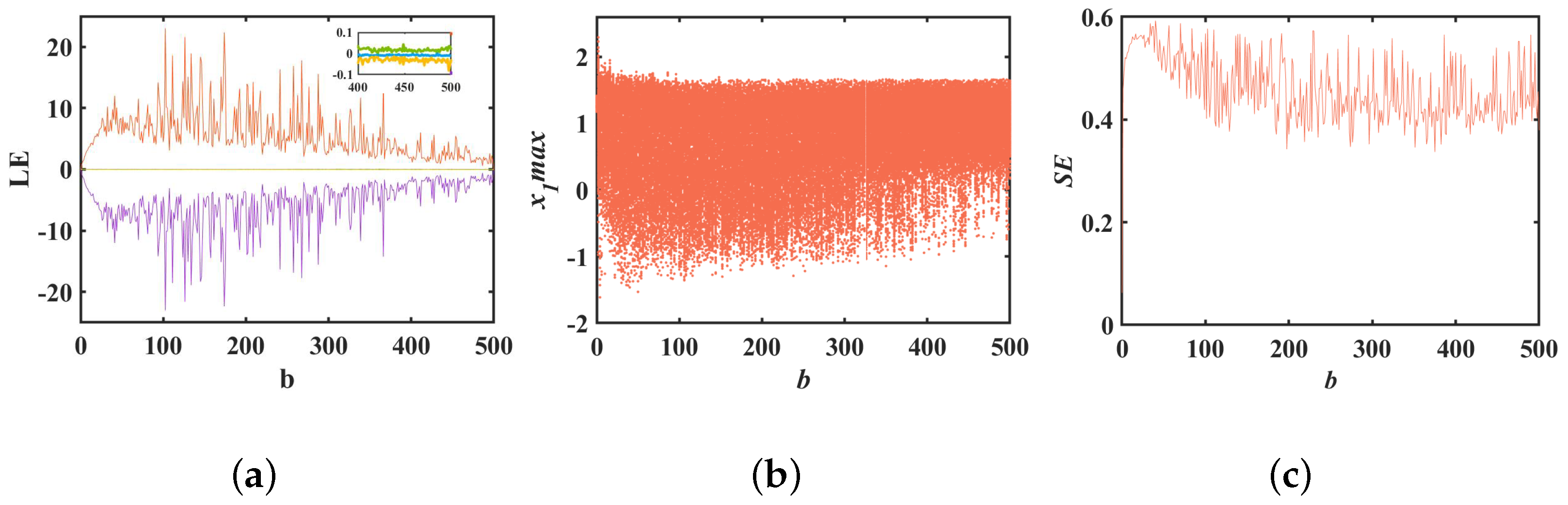
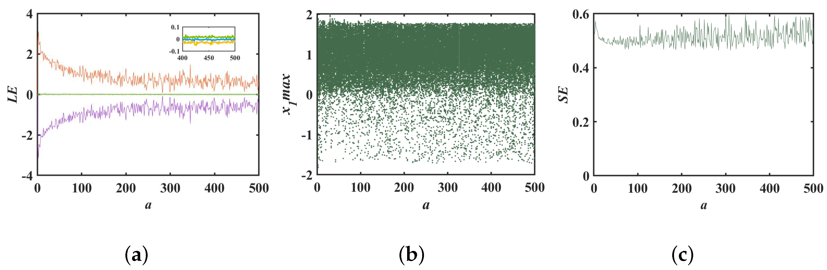
In Section 3.1, we observed that the maximum Lyapunov exponent of the system increases approximately linearly with the parameter b. This section delves into this phenomenon by maintaining constant system parameters at $a=10$, $k=2$, and initial values of $[1,1,1,1,1]$. The Lyapunov exponent and bifurcation diagrams for the varying parameter b are illustrated in Figure 5a,b. These diagrams reveal that the system maintains hyperchaotic behavior across a broad range of b values within $(0,500]$, without any periodic windows. The Lyapunov exponent diagram in Figure 5a indicates that the exponent in the first dimension generally rises with b in the interval $(0,180)$ and then shows a decreasing trend for b in $(180,500]$, yet it remains positive, indicating sustained hyperchaos. The point density in Figure 5b correlates with its Lyapunov exponent map; as the LE index increases, point density and coverage expand, and the pattern reverses as the index decreases. Our predictions suggest that once the system parameter b surpasses 500, the first-dimensional Lyapunov exponent will gradually decrease but the system’s conservative hyperchaos will persist, with its parameter range continuing to broaden. To quantify the complexity of chaotic sequences, the spectral entropy complexity (SE) variation concerning parameter b is plotted in Figure 5c. It is evident that the chaotic sequences generated by system (3) exhibit high structural complexity.

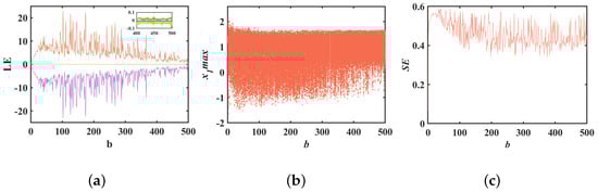
Figure 5. Bifurcation for parameter b: (a) Lyapunov exponential spectrum about b; (b) bifurcation diagram about b; (c) SE complexity about b.

This article further explores the impact of parameter a on the system’s bifurcation behavior. With system parameters $b=5$, $k=2$, and initial values $[1,1,1,1,1]$ held constant, Lyapunov exponent diagrams and bifurcation diagrams for various values of parameter a were plotted, as shown in Figure 6a,b. Unlike the influence of parameter b, the first-dimensional Lyapunov exponent of the system initially decreases with the increase of parameter a and then becomes stable. It can be observed from Figure 6b that within the interval $a\in (0,500]$ the point density distribution of the bifurcation diagram is more uniform, which is consistent with the trend observed in the Lyapunov exponent diagrams. The results of the spectral entropy map are consistent with the changes in the Lyapunov exponent diagrams and bifurcation diagrams, further corroborating the complexity of the system’s dynamic behavior.

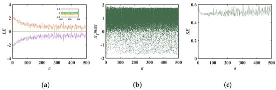
Figure 6. Bifurcation for parameter a: (a) Lyapunov exponential spectrum about a; (b) bifurcation diagram about a; (c) SE complexity about a.

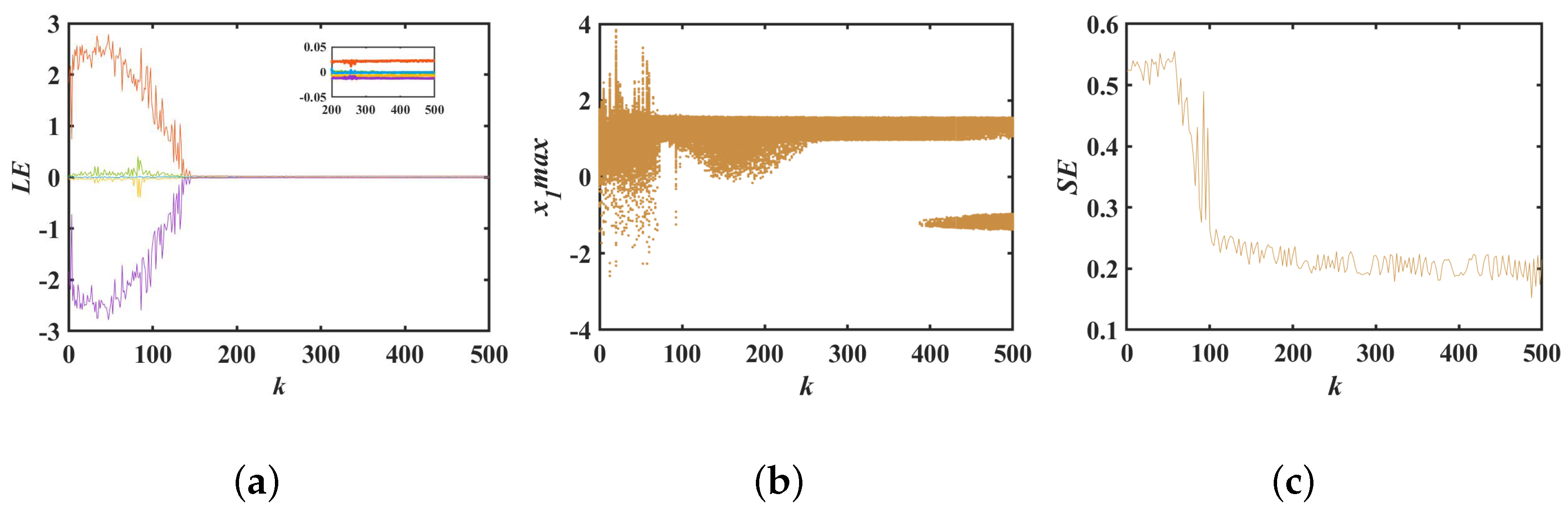
For comprehensiveness, this paper also analyzed the bifurcation behavior of parameter k. With the system parameters $a=10$, $b=5$, and the initial values $[1,1,1,1,1]$ held constant, Lyapunov exponent diagrams and bifurcation diagrams for various values of parameter k were plotted. It is evident from Figure 7a that as parameter k increases, the first-dimensional Lyapunov exponent declines rapidly, potentially giving rise to periodic windows. Figure 7b similarly indicates that the point density of the bifurcation diagram decreases, and that its coverage is significantly less compared to the bifurcation diagrams associated with parameters a and b. Considering the results of the spectral entropy diagram, to generate stable chaotic sequences the parameter range for k should be limited to $[0,80]$. Within this range, the system’s Lyapunov exponents are positive and there are no periodic windows.

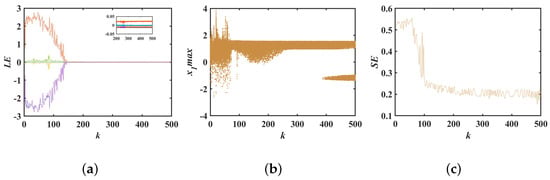
Figure 7. Bifurcation for parameter k: (a) Lyapunov exponential spectrum about k; (b) bifurcation diagram about k; (c) SE complexity about k.

Transient Quasi-Periodic

Transient chaos, a phenomenon observed in deterministic nonlinear dynamical systems, occurs due to the presence of a non-attractive chaotic saddle in phase space. This is characterized by a trajectory that, starting from random initial conditions, exhibits chaotic behavior for an extended period before abruptly transitioning to a periodic state [49]. Conversely, if a trajectory initially displays quasi-periodic motion and then suddenly transitions to chaos then this is referred to as transient quasi-periodicity [55].

In our prior analysis of the bifurcation behavior with respect to parameter k, we identified the system’s tendency towards transient quasi-periodicity. By setting the system parameters to $a=10$, $b=5$, $k=100$, and the initial values to $[1,1,1,1,1]$, we plotted the phase and time diagrams of system (3) for $t\in (0,500)$. These diagrams, depicted in Figure 8a,b, illustrate the system’s evolution from quasi-periodic to chaotic orbits. The combination of phase and time diagrams reveals that system (3) initially exhibits quasi-periodic orbits, as shown in Figure 8c. Subsequently, around $t=260$, these quasi-periodic orbits abruptly transition into stable chaotic orbits.

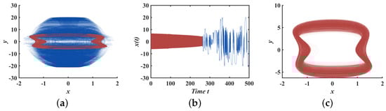
Figure 8. System (3) of $k=100$: (a) phase diagram of $k=100$; (b) time series of $t\in [0,500]$; (c) phase diagram of $t\in [0,260]$.

5. NIST Test

The NIST SP800-22 statistical test suite [56] is a statistical test suite published by the National Institute of Standards and Technology for evaluating and verifying the statistical performance of binary pseudo-random sequences generated by random number generators or pseudo-random number generators. The NIST test suite consists of 15 statistical tests that consider a variety of statistical characteristics from many different perspectives, to detect whether a sequence of random numbers is highly random. Depending on whether the test results pass their criteria, the feasibility and safety of the random number generator can be determined.

To obtain the binary sequence required for the measurement, it is necessary to first sample the chaotic orbit to obtain the real-valued sequence generated by the system. Assuming the sampling time is $T=0.01$, the initial the values of system (3) are then set to $(1,1,1,1,1)$ to obtain the chaotic orbit, which is subsequently truncated. Sampling is then performed at the specified sampling interval, to obtain a 5D sequence $x\left(t\right),y\left(t\right),z\left(t\right),w\left(t\right),u\left(t\right)$. Finally, a simple encoding algorithm is applied, to transform the five-dimensional chaotic sequence into a binary sequence.

For this section, the chaotic random sequence $\left\{S\right\}$ generated based on system (3) was tested for randomness and uniformity through NIST tests.

A binary sequence $\left\{S\right\}$ of size ${10}^6$ bits was generated based on system (3), and $\left\{S\right\}$ was divided equally into $n=100$ groups, each containing a binary sequence of size 106 bits. The test yielded the $P-value$, as well as the pass ratio of each group of sequences, and then the corresponding $P-valu{e}_T$ was calculated by Equation (11):

$$\left\{\begin{array}{c}P-valu{e}_T=igamc({\displaystyle \frac{9}{2}},{\displaystyle \frac{x^2}{2}})\hfill \\ x^2=\sum _{i=1}^{10}={\displaystyle \frac{{\left(F_i-(s/10)\right)}^2}{s/10}}\hfill \end{array}\right.$$

(11)

where $igamc$ is the incomplete gamma function, $F_i$ is the number of values in subinterval i, and s is the sample size.

If the test results satisfied the following three test requirements at the same time, it indicated that the sequence passed the test in statistical significance and had good randomness:

(a) Each should be greater than the $\alpha =0.01$ predefined significance level.

(b) Each corresponding pass rate should lie within the confidence interval $(\widehat{p}-3\sqrt{{\displaystyle \frac{\widehat{p}(1-\widehat{p})}{n}}},(\widehat{p}+3\sqrt{{\displaystyle \frac{\widehat{p}(1-\widehat{p})}{n}}}))$, where $\widehat{p}=1-\alpha$. The confidence interval should be calculated to be (0.9601, 1.0298).

(c) Each p-Value_T should be greater than 0.0001.

The full test results are shown in Table 3. For items with more tests, there were multiple p-Values in the test results, and only the smallest p-Value among all the items is listed in Table 3. If the smallest p-Value passed the test, it could be proved that the item passed every test. As can be seen in Table 3, the p-value, the passing percentage, and the $p-Valu{e}_T$ all satisfied the above three test requirements, and the pseudo-random number sequences generated in this chapter passed all the NIST tests.

Table 3. Nist test result.

No.	Statistical Test	p-Value	Proportion	p-ValueT	Result
1	Frequency	0.455937	0.98	0.5818	✓
2	Block Frequency	0.699313	0.99	0.7363	✓
3	Cumulative Sums	0.289667	0.99	0.3954	✓
4	Runs	0.534146	0.99	0.6577	✓
5	Longest Run	0.089121	1	0.9121	✓
6	Rank	0.867692	0.98	0.9121	✓
7	FFT	0.719747	0.99	0.8116	✓
8	Non-Overlapping Template	0.019188	0.98	0.0186	✓
9	Universal	0.637119	0.98	0.8257	✓
10	Approximate Entropy	0.883171	1	0.9217	✓
11	Random Excursions	0.000533	1	0.0003	✓
12	RandomExcursionsVariant	0.001313	0.99	0.0007	✓
13	Overlapping Template	0.350485	1	0.4678	✓
14	Serial	0.090936	1	0.1224	✓
15	Linear Complexity	0.383827	1	0.5054	✓

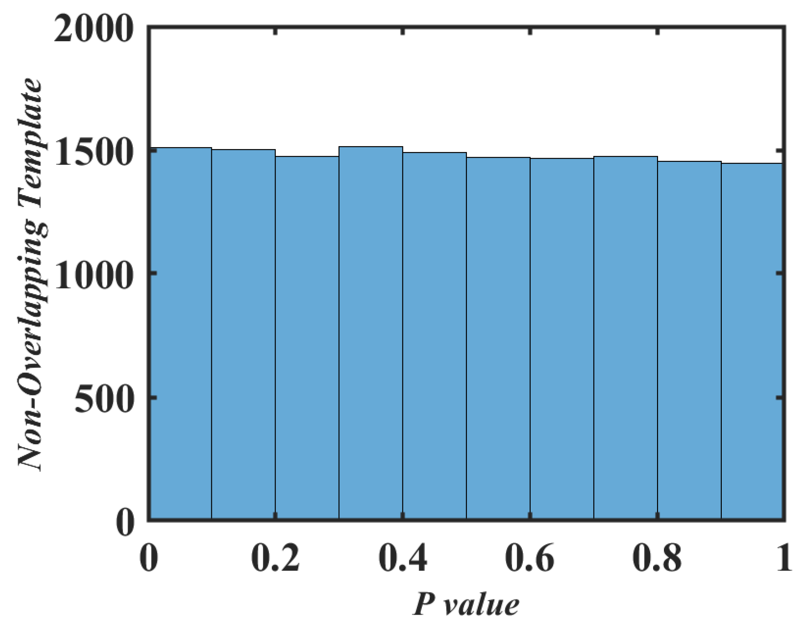
In addition, in order to observe the distribution of the p-Values more intuitively and assess the uniformity of the sequence, Figure 9 shows a histogram of the distribution of the p-Values in non-overlapping template matching detection. As can be seen from Figure 9, the distribution of the p-Values was very uniform. Therefore, the pseudo-random number sequence generated based on system (3) successfully passed all the NIST tests with good randomness and uniformity.

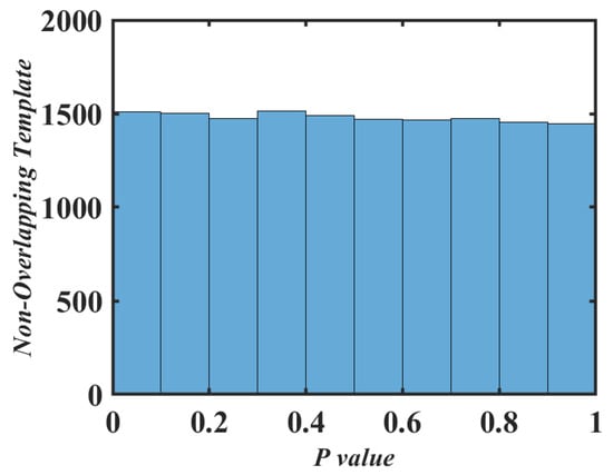
Figure 9. The non-overlapping template p-value histogram.

6. Image-Encryption Application

In recent years, with the advancement of chaos theory, chaos-based image-encryption algorithms have shone in the field of image encryption, due to their rich and complex dynamic behaviors and high sensitivity to initial values.

In nonlinear dynamical systems, the fundamental difference between CCSs and DCSs lies in the fact that the former do not have attractors, which provides unique advantages for image encryption [44,57]. CCSs maintain the constancy of phase space volume, unlike dissipative systems that tend towards one or more attractors, thereby reducing the predictability and reconstructability of the system’s state. Since image encryption requires algorithms to have a high degree of unpredictability and sensitivity, the characteristics of CCSs can effectively resist cryptographic attacks based on attractor analysis, enhancing the security of the encryption process. Therefore, when designing image-encryption algorithms, CCSs are considered a more ideal choice, due to their unique dynamic characteristics.

6.1. Image-Encryption Process

In a 256-level grayscale image, each pixel’s grayscale value is represented by 8 binary bits. By sequentially extracting each pixel’s bits, 8-bit planes can be formed. Specifically, the 1st plane contains the least significant bit of all the pixels in the image, while the 8th plane contains the most significant bit. By layering the image, a chaotic sequence generated by the 5D CMHS is used to encrypt each bit plane of the image individually. The specific encryption process is as follows:

step1: Select a grayscale image of $M\times N$ pixels, represented in binary form, as the raw image to be processed, and decompose it into eight-bit planes. Then, perform a scrambling operation on the higher-order bit planes, namely, the 5th, 6th, 7th, and 8th bit planes.

step2: Utilize the fourth-order classical Runge–Kutta method to iterate the 5D CMHS, generating a chaotic sequence. From the state variables x and y, generate five sets of $M\times N$-sized chaotic sequences, $X_n$ and $Y_n$, and from the state variables z and w generate two sets of $M\times N$-sized chaotic sequences, $Z_n$ and $W_n$. Then, discard the first set of $M\times N$ chaotic sequences from each group, to reduce the influence of the initial conditions. The remaining four sets are used for permutation operations, and the remaining one set is used for diffusion operations.

step3: Using Equation (13), perform Arnold scrambling on the bit planes 5, 6, 7, and 8. Here, $(i,j)$ denotes the initial pixel position of the image, and $(p,q)$ represents the scrambled pixel position after the operation. Since pixel positions must be integers, the floating-point chaotic sequence generated by the chaotic system needs to be converted to integers. Then, use Equation (12) to extract the values of a and b from the chaotic sequences $X_n$ and $Y_n$. After the scrambling operation, the image must be reshaped to ensure that the dimensions and structure of the image remain unchanged:

$$\begin{array}{c}\hfill a=\mathrm{round}(X_{n}modN)\\ \hfill b=\mathrm{round}(Y_{n}modN)\\ \hfill \end{array}$$

(12)

Here, N is the size of the image, and round is the rounding function, ensuring that a and b are integers:

$$\left[\begin{array}{c}p\\ q\end{array}\right]=\left[\begin{array}{cc}1& a\\ b& ab+1\end{array}\right]\left[\begin{array}{c}i\\ j\end{array}\right]mod\left.[\begin{array}{c}M\\ N\end{array}\right]+\left[\begin{array}{c}1\\ 1\end{array}\right]$$

(13)

where M and N represent the height and width of the image, respectively, and mod denotes the modulo operation to ensure that the pixel positions are within the boundaries of the image.

step4: To enhance the encryption effect, it is necessary to perform diffusion operations on the scrambled image. Equation (14) is used to perform modular arithmetic and circular left-shift diffusion on the scrambled image, effectively improving the encryption effect:

$$C_i=(C_{i-1}+S_i+P_i+H\left(P_{1:i}\right))mod256<<<LS{B}_3\left(C_{i-1}\right)$$

(14)

Here, P represents the scrambled image, C and S are the key sequences extracted from the chaotic sequences $Z_n$ and $W_n$, $H\left(P_{1:i}\right)$ represents the hash value of the first i pixels, ensuring that local changes affect all subsequent pixels, and $LS{B}_3$ indicates a circular left-shift operation on the lowest 3 bits of the data.

The decryption process is the reverse of the encryption process, as shown in Figure 10:

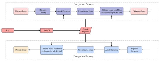
Figure 10. Image-encryption and -decryption algorithm flowchart.

6.2. Performance and Security Analysis

6.2.1. Histogram Analysis

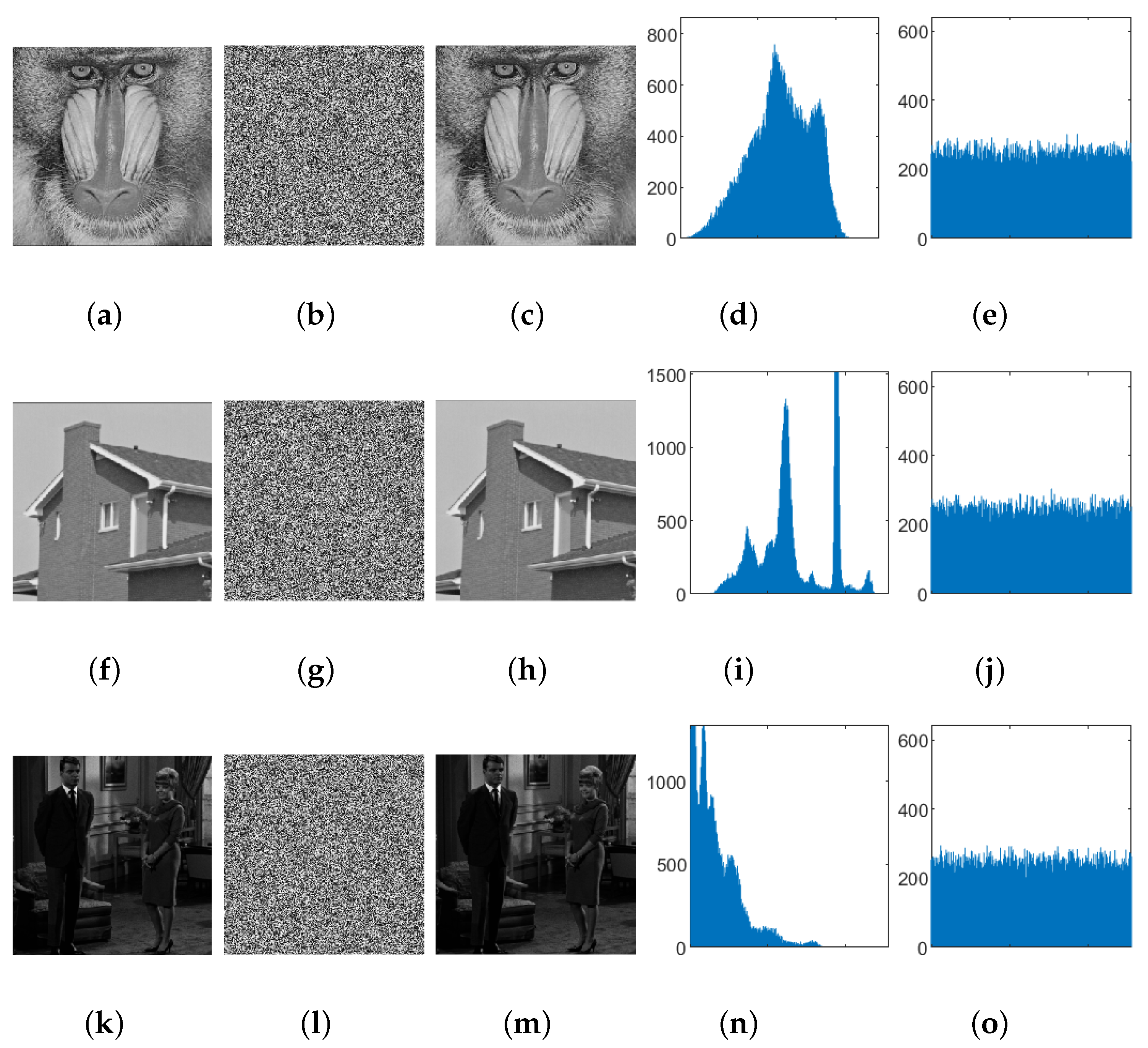
The histogram represents the quantity of pixel values in an image. An encrypted image with an ideal histogram distribution is uniform, and it can effectively resist attacks. We selected three sets of images for testing, and the results are shown in Figure 11. Figure 11a,f,k are the original images, and the encrypted result images are shown as Figure 11b,g,l. Figure 11c,h,m are the decrypted images. Figure 11c,h,m are the histograms of the three sets of original images, and Figure 11e,j,o are the histograms of the encrypted images.

Figure 11. Baboon’s (a) original image, (b) encrypted image, (c) decrypted image. House’s (f) original image, (g) encrypted image, (h) decrypted image. Men’s (k) original image, (l) encrypted image, (m) decrypted image. Histogram of the original image: (d) Baboon, (i) House, (n) Men. Histogram of encrypted images: (e) Baboon, (j) House, (o) Men.

According to Figure 11, visually the ciphertext image has a flat histogram, while the histogram of the plaintext image fluctuates; the ${\chi }^2$ statistic (one-tailed hypothesis test) is often used to quantitatively measure the difference between the two. For a grayscale image with 256 levels of gray, let the size of the image be $M\times N$, and assume that the frequency of each gray level $f_i$ in its histogram follows a uniform distribution, which is $g_i$ = g = $MN/256$, i = 0, 1, 2, …, 255; then,

$${\chi }^2=\sum _{i=0}^{255}{\displaystyle \frac{{(f_i-g)}^2}{g}}$$

(15)

follows a ${\chi }^2$ distribution with 255 degrees of freedom. Given a significance level $\alpha$, this ensures that

$$P\left\{{\chi }^2\ge {\chi }_a^2\left(n-1\right)\right\}=\alpha$$

(16)

The commonly used significance level $\alpha$ is 0.05; thus, we have ${\chi }_{0.05}^{\left(255\right)}=293.24783$. From Table 4, it can be seen that the test statistic value of the original image is significantly greater than ${\chi }_{0.05}^{\left(255\right)}$, while the test statistic values of the ciphertext images are all less than ${\chi }_{0.05}^{\left(255\right)}$. It can be considered that at a significance level of 0.05 the histogram distribution of the ciphertext image is approximately uniform.

Table 4. Test result for ${\chi }^2$.

Index	Plain Image			Cipher Image
	Baboon	House	Men	Baboon	House	Men
result	$5.438\times {10}^4$	$3.006\times {10}^5$	$2.183\times {10}^5$	$208.484$	$209.273$	$238.766$

6.2.2. Key Space Analysis

In cryptography, the key space refers to the set of all possible keys, and its size directly determines the robustness of a cryptographic system against attacks. The larger the key space, the more effective it is in resisting exhaustive attacks. The algorithm proposed in this paper generates a 32-bit binary chaotic sequence as the key, based on the initial conditions $(x_0,y_0,z_0,w_0,u_0)$, yielding a key space of $2^{160}$, which is significantly larger than the commonly accepted security threshold of $2^{128}$. Given the key space of $2^{160}$, the algorithm can effectively withstand external exhaustive attacks.

6.2.3. Correlation Analysis of Adjacent Pixels

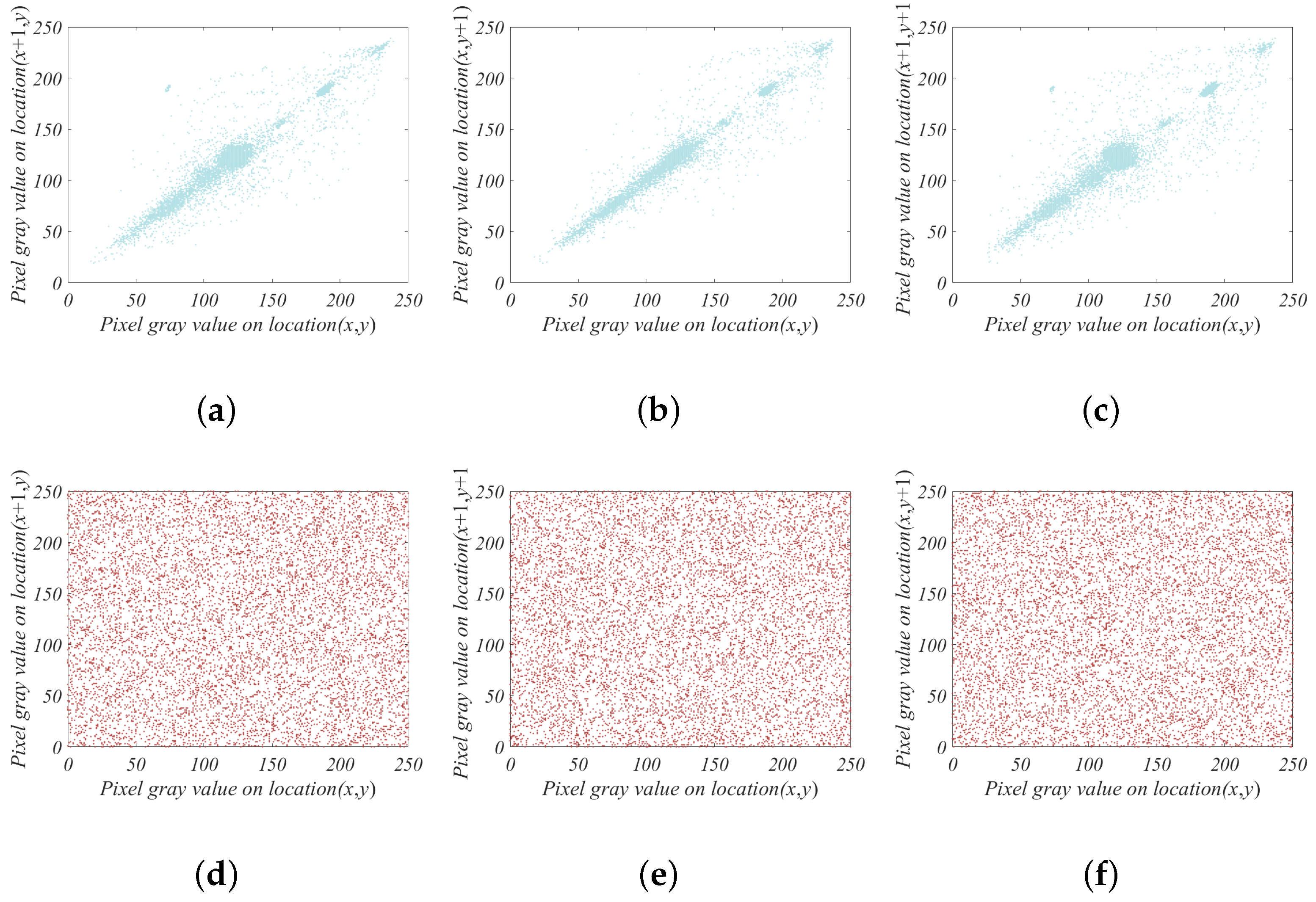
In addition to the image histogram, it is also necessary to compare the correlation characteristics between the plaintext image and its ciphertext image. Generally, plaintext images have strong correlations between adjacent pixel points in horizontal, vertical, and diagonal directions, while there should be no correlation between adjacent pixel points in the ciphertext image.

Let N pairs of adjacent pixels be randomly selected from the original image, and their grayscale values are denoted as $(u_i,v_i)$, where i = 1, 2, 3,…, N. The correlation coefficient between the vectors u = $\left\{u_i\right\}$ and v = $\left\{v_i\right\}$ is calculated using the following formula:

$$\begin{array}{cc}\hfill & r_{xy}={\displaystyle \frac{\mathrm{cov}(u,v)}{\sqrt{D\left(u\right)}\sqrt{D\left(v\right)}}}\hfill \\ \hfill & cov(u,v)={\displaystyle \frac{1}{N}}\sum _{i=1}^N(x_i-E\left(u\right))(y_i-E\left(v\right))\hfill \\ \hfill & D\left(u\right)={\displaystyle \frac{1}{N}}\sum _{{\displaystyle \genfrac{}{}{0pt}{}{i=1}{N}}}^N{\left(u_i-E\left(u\right)\right)}^2\hfill \\ \hfill & E\left(u\right)={\displaystyle \frac{1}{N}}\sum _{i=1}{u}_i\hfill \end{array}$$

(17)

Taking the House image as an example, the calculation results are shown in Table 5. From Table 5, it can be seen that the correlation between adjacent pixel points in the plaintext image is quite strong, while the correlation between adjacent pixel points in the ciphertext image is close to 0, indicating almost no correlation. Figure 12 illustrates the correlation between adjacent pixels in the horizontal, vertical, and diagonal directions for both the plaintext and ciphertext images of the House. It can be observed from the figure that the pairs of adjacent pixels in the plaintext image are concentrated on the line $y=x$ in all directions, whereas the pairs of pixels in the ciphertext image are uniformly distributed in a rectangular pattern. This corroborates the results shown in Table 5, indicating that the algorithm has a good encryption effect.

Table 5. Correlation analysis of adjacent pixels.

Image	Horizontal	Vertical	Angle
Plain Image	0.9532	0.9768	0.9336
ours	0.0075	−0.0031	0.0016
Ref. [58]	0.1539	0.1342	−0.0277
Ref. [59]	−0.0290	−0.0166	−0.0029

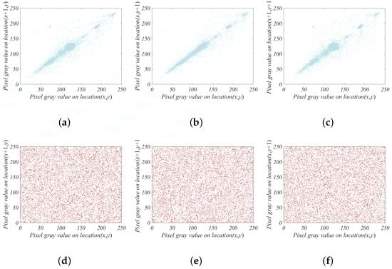
Figure 12. Scatter diagrams of adjacent pixel correlation of House image. Original image correlation diagram in (a) horizontal direction, (b) vertical direction, (c) angle direction. Cipher image correlation diagram in (d) horizontal direction, (e) vertical direction, (f) angle direction.

6.2.4. Information Entropy

Information entropy reflects the uncertainty of image information. It is generally believed that the higher the information entropy, the greater the uncertainty, the richer the amount of information contained, and the less readable the information in the image. The calculation formula for information entropy is as follows:

$$H=-\sum _{i=0}^{L}p\left(i\right){\log }_{2}p\left(i\right)$$

(18)

In the formula, L represents the number of gray levels in the image, and $p\left(i\right)$ denotes the probability of the occurrence of the gray value i.

As shown in Table 6, the experimental results of information entropy for plaintext and encrypted images were compared, and the encryption algorithm proposed in this paper was contrasted with the existing literature. The results indicate that the information entropy of the encryption algorithm proposed in this paper is closer to the theoretical maximum value of 8, thereby confirming its superior encryption effectiveness.

Table 6. The results of information entropy.

Image	Plain	Cipherl	Ref. [60]	Ref. [61]	Ref. [62]
Information entropy	7.2925	7.9977	7.991	7.906	7.740

6.2.5. Key Sensitivity Analysis

In the field of image encryption, key sensitivity analysis is an important metric. Key sensitivity refers to the situation where a slight change in the key results in a significant difference between the two encrypted images obtained, indicating that the algorithm has strong key sensitivity. Conversely, if the difference is small, it is considered to have weak key sensitivity. The NPCR and the UACI are two common indicators used to measure key sensitivity. The NPCR measures the proportion of different pixel points when the key changes slightly, calculated by the following formula:

$$NPCR(P_1,P_2)={\displaystyle \frac{1}{MN}}\sum _{i=1}^M\sum _{j=1}^N\left|Sign(P_1(i,j)-P_2(i,j))\right|\times 100\%$$

(19)

The UACI assesses key sensitivity by calculating the average value of entropy differences at each pixel position between two images. The calculation formula is as follows:

$$UACI(P_1,P_2)={\displaystyle \frac{1}{MN}}\sum _{\mathrm{i}}^M\sum _j^N{\displaystyle \frac{\left|P_1(i,j)-P_2(i,j)\right|}{255-0}}\times 100\%$$

(20)

The key for this image-encryption algorithm is the initial value of the 5D CMHS, which is $K=\{x_0,y_0,z_0,w_0,u_0\}$. By slightly changing the initial values $\left({10}^{-13}\right)$ and encrypting the same image again, we obtained two cipher images. Finally, we calculated their NPCR and UACI values. The calculation results are shown in Table 7. As the table shows, the calculation results are close to the theoretical values:

Table 7. Coefficient of association.

Index	${\mathit{x}}_0$	${\mathit{y}}_0$	${\mathit{z}}_0$	${\mathit{w}}_0$	${\mathit{u}}_0$	Theoretical Value
NPCR	99.5804	99.5651	99.6094	99.6002	99.6338	99.6094
UACI	33.0076	33.4736	33.2926	33.3650	33.5402	33.4635

6.2.6. Plain Image Sensitivity Analysis

Plaintext sensitivity refers to the degree of change in the ciphertext image output by the encryption algorithm when minor changes occur in the plaintext image. An excellent encryption algorithm should be highly sensitive to input, meaning that even minor changes in the plaintext image will result in significant differences in the output ciphertext image. Such minor differences can be achieved by altering a few pixel points in the plaintext image. For example, by randomly selecting a pixel point $P_{(}i,j)$ from the plaintext image and changing its value, the variation is set to 1, i.e., the changed value is $(P_{(}i,j)+1)$$mod$ 256, and an almost imperceptible change in the plaintext image can be obtained. The results of the plaintext sensitivity analysis are shown in Table 8. The results indicate that both the NPCR and UACI values are close to their ideal values; hence, the image-encryption system based on 5D CMHS can effectively resist plaintext attacks.

Table 8. The results of plain image sensitivity analysis.

Index	Baboon	House	Men	Theoretical Value
NPCR	99.5850	99.6338	99.6338	99.6094
UACI	33.2926	33.4629	33.4481	33.4635

6.2.7. Noise Attacks and Data-Loss Attacks Analysis

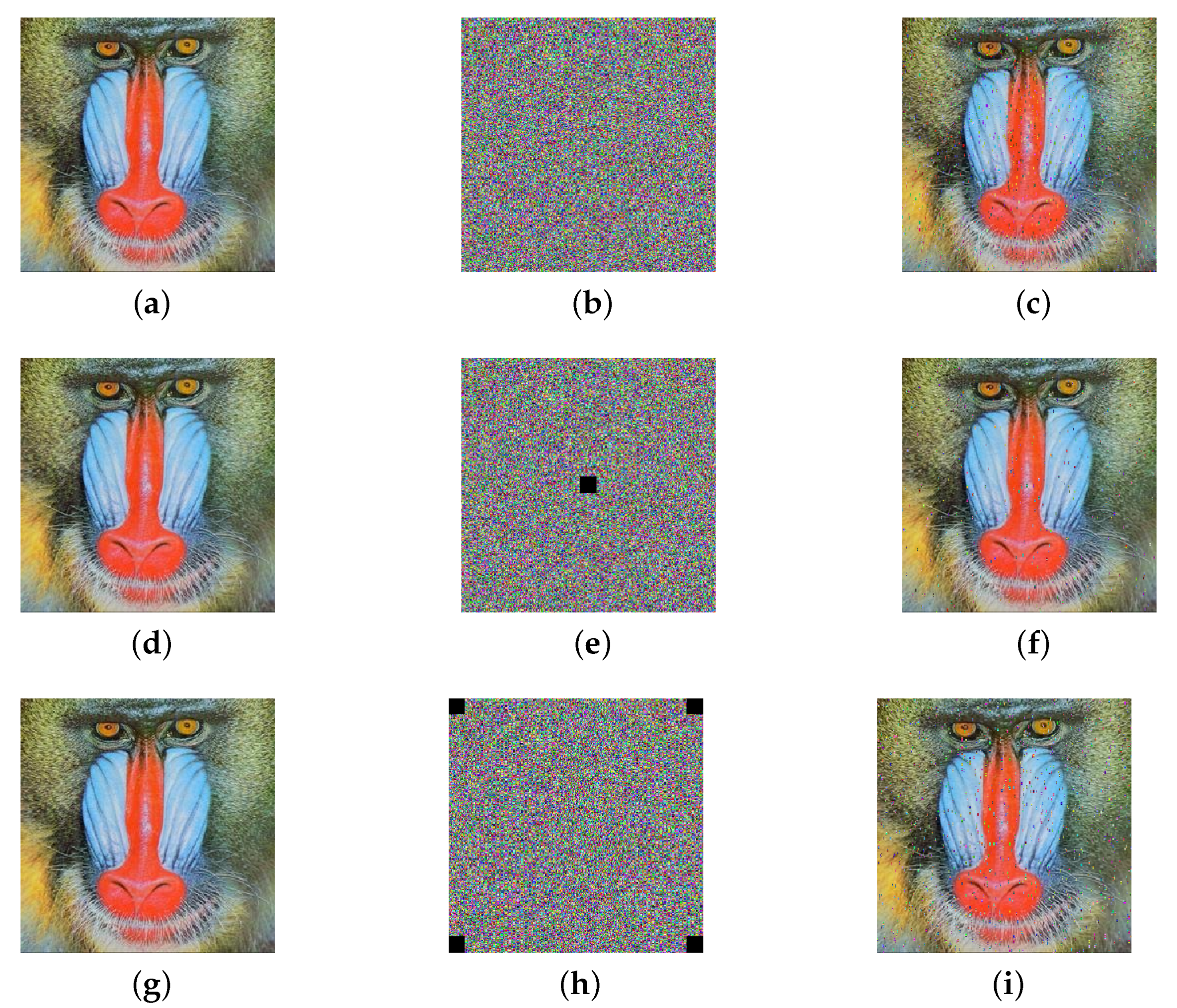
In the field of image encryption, noise attacks and data-loss attacks are two common threats. They aim to compromise the integrity and confidentiality of encrypted images by introducing noise or deleting parts of the data. Although some algorithms may exhibit remarkable statistical properties, they may still fall short in terms of cryptographic security. Therefore, taking the Baboon image as an example, this study comprehensively evaluated the proposed encryption algorithm by introducing salt-and-pepper noise attacks, corner-cropping attacks, and center-cropping attacks.

As depicted in Figure 13b,e,h, we subjected the encrypted images to salt-and-pepper noise attacks, center-cropping attacks, and corner-cropping attacks, respectively. The results indicate that, despite these attacks, the algorithm was still able to decrypt the images fairly intact, as shown in Figure 13c,f,i. This demonstrates that the algorithm has superior performance, in terms of noise resistance and data loss resistance, and that it is capable of effectively withstanding noise attacks and data-loss attacks, thereby providing more reliable security guarantees in practical applications.

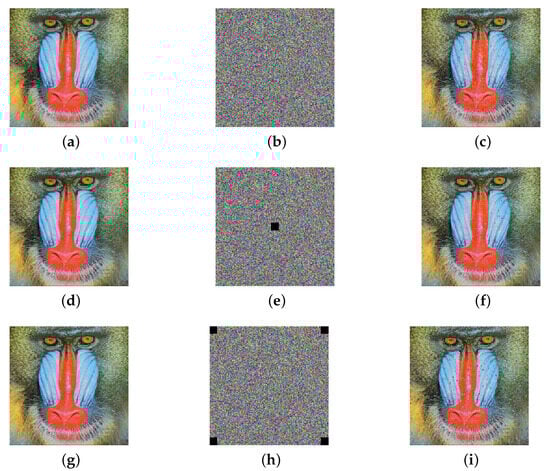
Figure 13. Noise attacks and data-loss attacks on Baboon image: (a,d,g) Baboon’s original image, (b) salt = 0.005, (c) salt-decrypted image, (e) center-cropping attack, (f) center-cropping attack decrypted image, (h) periphery-cropping attack, (i) periphery-cropping attack decrypted image.

6.2.8. Time Complexity Analysis

Time complexity analysis is a crucial metric for evaluating the practicality of encryption algorithms, especially in scenarios with high real-time requirements, where algorithms need to complete complex computations within a reasonable timeframe. In this study, standard test images with resolutions of $256\times 256$ and $512\times 512$ pixels were used, and the results are shown in Table 9. The encryption time for the $256\times 256$ image was 1.41 s, while that for the $512\times 512$ image was 5.36 s. The increase in time consumption was primarily due to the expansion of the key space through the high-dimensional characteristics and broad parameter range of the five-dimensional chaotic system, which increased the computational load for generating chaotic sequences and involved multiple iterations in the scrambling and diffusion phases. Although the time cost increased, the algorithm still maintained high efficiency. The experimental results demonstrate that the proposed algorithm achieves a balanced optimization between encryption speed and attack resistance by trading off complexity and security, meeting real-time requirements.

Table 9. The results of encryption and decryption speed.

Image Size	Encryption	Decryption
$256\times 256$	1.41	1.43
$512\times 512$	5.36	5.34

7. Conclusions

This paper introduces a novel 5D CMHS based on the combination of a 4D CCS and memristors. The system demonstrates stable conservative chaotic characteristics and superior ergodicity over a broad range of parameters. Additionally, the system exhibits multi-stability, allowing for the co-existence of multiple hyperchaotic trajectories within a wide range of initial values. Furthermore, through divergence, phase diagrams, equilibrium points, and LEs, it has been proven that the system is a conservative hyperchaotic system, characterized by zero attractors, zero divergence, zero-sum of LEs, integer dimensions, and equilibrium points that are solely saddle points, which collectively validate its nature as a conservative hyperchaotic system. By spectral entropy complexity analysis and NIST testing, it has been shown that the chaotic sequences generated by the new system possess high complexity and good pseudorandomness. Ultimately, based on the proposed novel system, an image-encryption algorithm has been developed. Through a rigorous security analysis, the feasibility of this image-encryption algorithm has been demonstrated, establishing its potential for practical application.

References

- Deng, Q.; Wang, C.; Sun, Y.; Deng, Z.; Yang, G. Memristive Tabu Learning Neuron Generated Multi-Wing Attractor With FPGA Implementation and Application in Encryption. IEEE Trans. Circuits Syst. I Regul. Pap. 2025, 72, 300–311. [Google Scholar] [CrossRef]
- Feng, W.; Yang, J.; Zhao, X.; Qin, Z.; Zhang, J.; Zhu, Z.; Wen, H.; Qian, K. A Novel Multi-Channel Image Encryption Algorithm Leveraging Pixel Reorganization and Hyperchaotic Maps. Mathematics 2024, 12, 3917. [Google Scholar] [CrossRef]
- Yu, F.; Su, D.; He, S.; Wu, Y.; Zhang, S.; Yin, H. Resonant tunneling diode cellular neural network with memristor coupling and its application in police forensic digital image protection. Chin. Phys. B 2025. [Google Scholar] [CrossRef]
- Wang, C.; Luo, D.; Deng, Q.; Yang, G. Dynamics analysis and FPGA implementation of discrete memristive cellular neural network with heterogeneous activation functions. Chaos Solitons Fractals 2024, 187, 115471. [Google Scholar] [CrossRef]
- Deng, W.; Ma, M. Analysis of the dynamical behavior of discrete memristor-coupled scale-free neural networks. Chin. J. Phys. 2024, 91, 966–976. [Google Scholar] [CrossRef]
- Li, J.; Wang, C.; Deng, Q. Symmetric multi-double-scroll attractors in Hopfield neural network under pulse controlled memristor. Nonlinear Dyn. 2024, 112, 14463–14477. [Google Scholar] [CrossRef]
- Zhu, J.; Jin, J.; Chen, C.; Wu, L.; Lu, M.; Ouyang, A. A New-Type Zeroing Neural Network Model and Its Application in Dynamic Cryptography. IEEE Trans. Emerg. Top. Comput. Intell. 2025, 9, 176–191. [Google Scholar] [CrossRef]
- Luo, D.; Wang, C.; Deng, Q.; Sun, Y. Dynamics in a memristive neural network with three discrete heterogeneous neurons and its application. Nonlinear Dyn. 2024, 113, 5811–5824. [Google Scholar] [CrossRef]
- Yu, F.; Lin, Y.; Yao, W.; Cai, S.; Lin, H.; Li, Y. Multiscroll hopfield neural network with extreme multistability and its application in video encryption for IIoT. Neural Netw. 2025, 182, 106904. [Google Scholar] [CrossRef]
- Yu, F.; Xu, S.; Lin, Y.; Gracia, Y.M.; Yao, W.; Cai, S. Dynamic Analysis, Image Encryption Application and FPGA Implementation of a Discrete Memristor-Coupled Neural Network. Int. J. Bifurc. Chaos 2024, 34, 2450068. [Google Scholar] [CrossRef]
- Zhu, S.; Deng, X.; Zhang, W.; Zhu, C. Construction of a new 2D hyperchaotic map with application in efficient pseudo-random number generator design and color image encryption. Mathematics 2023, 11, 3171. [Google Scholar] [CrossRef]
- Yu, F.; Zhang, W.; Xiao, X.; Yao, W.; Cai, S.; Zhang, J.; Wang, C.; Li, Y. Dynamic analysis and field-programmable gate array implementation of a 5D fractional-order memristive hyperchaotic system with multiple coexisting attractors. Fractal Fract. 2024, 8, 271. [Google Scholar] [CrossRef]
- Wan, Q.; Liu, J.; Liu, T.; Sun, K.; Qin, P. Memristor-based circuit design of episodic memory neural network and its application in hurricane category prediction. Neural Netw. 2024, 174, 106268. [Google Scholar] [CrossRef] [PubMed]
- Lai, Q.; Yang, L.; Chen, G. Design and Performance Analysis of Discrete Memristive Hyperchaotic Systems With Stuffed Cube Attractors and Ultraboosting Behaviors. IEEE Trans. Ind. Electron. 2024, 71, 7819–7828. [Google Scholar] [CrossRef]
- Gao, X.L.; Zhang, H.L.; Wang, Y.L.; Li, Z.Y. Research on Pattern Dynamics Behavior of a Fractional Vegetation-Water Model in Arid Flat Environment. Fractal Fract. 2024, 8, 264. [Google Scholar] [CrossRef]
- Chen, G.; Ueta, T. Yet another chaotic attractor. Int. J. Bifurc. Chaos 1999, 9, 1465–1466. [Google Scholar] [CrossRef]
- Anishchenko, V.S.; Safonova, M.; Chua, L.O. Stochastic resonance in Chua’s circuit. Int. J. Bifurc. Chaos 1992, 2, 397–401. [Google Scholar] [CrossRef]
- Lü, J.; Chen, G. A new chaotic attractor coined. Int. J. Bifurc. Chaos 2002, 12, 659–661. [Google Scholar] [CrossRef]
- Sprott, J.C. Some Simple Chaotic Flows. Phys. Rev. E 1994, 50, R647–R650. [Google Scholar] [CrossRef]
- Lorenz, E.N. Deterministic Nonperiodic Flow. J. Atmos. Sci. 1963, 20, 130–141. [Google Scholar] [CrossRef]
- Ji’e, M.; Yan, D.; Sun, S.; Zhang, F.; Duan, S.; Wang, L. A Simple Method for Constructing a Family of Hamiltonian Conservative Chaotic Systems. IEEE Trans. Circuits Syst. I Regul. Pap. 2022, 69, 3328–3338. [Google Scholar] [CrossRef]
- Liu, X.; Tong, X.; Wang, Z.; Zhang, M. Construction of Controlled Multi-Scroll Conservative Chaotic System and Its Application in Color Image Encryption. Nonlinear Dyn. 2022, 110, 1897–1934. [Google Scholar] [CrossRef]
- Yuan, Y.; Yu, F.; Tan, B.; Huang, Y.; Yao, W.; Cai, S.; Lin, H. A class of n-D Hamiltonian conservative chaotic systems with three-terminal memristor: Modeling, dynamical analysis, and FPGA implementation. Chaos 2025, 35, 013121. [Google Scholar] [CrossRef] [PubMed]
- Cang, S.; Wu, A.; Wang, Z.; Chen, Z. Four-Dimensional Autonomous Dynamical Systems with Conservative Flows: Two-Case Study. Nonlinear Dyn. 2017, 89, 2495–2508. [Google Scholar] [CrossRef]
- Leng, X.; Gu, S.; Peng, Q.; Du, B. Study on a Four-Dimensional Fractional-Order System with Dissipative and Conservative Properties. Chaos Solitons Fractals 2021, 150, 111185. [Google Scholar] [CrossRef]
- Leng, X.; Du, B.; Gu, S.; He, S. Novel Dynamical Behaviors in Fractional-Order Conservative Hyperchaotic System and DSP Implementation. Nonlinear Dyn. 2022, 109, 1167–1186. [Google Scholar] [CrossRef]
- Tian, B.; Peng, Q.; Leng, X.; Du, B. A New 5D Fractional-Order Conservative Hyperchaos System. Phys. Scr. 2023, 98, 015207. [Google Scholar] [CrossRef]
- Fu, H.; Lei, T. Adomian Decomposition, Dynamic Analysis and Circuit Implementation of a 5D Fractional-Order Hyperchaotic System. Symmetry 2022, 14, 484. [Google Scholar] [CrossRef]
- Ye, X.; Wang, X. Characteristic Analysis of a Simple Fractional-Order Chaotic System with Infinitely Many Coexisting Attractors and Its DSP Implementation. Phys. Scr. 2020, 95, 075212. [Google Scholar] [CrossRef]
- Marsden, J.E.; Ratiu, T.S. Introduction to Mechanics and Symmetry: A Basic Exposition of Classical Mechanical Systems; Springer Science & Business Media: New York, NY, USA, 2013; Volume 17. [Google Scholar]
- Ning, X.; Dong, Q.; Zhou, S.; Zhang, Q.; Kasabov, N.K. Construction of New 5D Hamiltonian Conservative Hyperchaotic System and Its Application in Image Encryption. Nonlinear Dyn. 2023, 111, 20425–20446. [Google Scholar] [CrossRef]
- Qi, G. Modelings and Mechanism Analysis Underlying Both the 4D Euler Equations and Hamiltonian Conservative Chaotic Systems. Nonlinear Dyn. 2019, 95, 2063–2077. [Google Scholar] [CrossRef]
- Pan, H.; Li, G.; Gu, Y.; Wu, S. Construction method and circuit design of a high-dimensional conservative chaotic system with binary linear combinations. Nonlinear Dyn. 2024, 112, 16495–16518. [Google Scholar] [CrossRef]
- Sprott, J.C. Elegant Chaos: Algebraically Simple Chaotic Flows; World Scientific: Singapore, 2010. [Google Scholar]
- Gugapriya, G.; Rajagopal, K.; Karthikeyan, A.; Lakshmi, B. A Family of Conservative Chaotic Systems with Cyclic Symmetry. Pramana 2019, 92, 48. [Google Scholar] [CrossRef]
- Zhang, Z.; Huang, L.; Liu, J.; Guo, Q.; Du, X. A New Method of Constructing Cyclic Symmetric Conservative Chaotic Systems and Improved Offset Boosting Control. Chaos Solitons Fractals 2022, 158, 112103. [Google Scholar] [CrossRef]
- Zhang, Z.; Huang, L.; Liu, J.; Guo, Q.; Li, C. Exploring Extreme Multistability in Cyclic Symmetric Conservative Systems via Two Distinct Methods. Nonlinear Dyn. 2024, 112, 10509–10528. [Google Scholar] [CrossRef]
- Gu, S.; Du, B.; Wan, Y. A New Four-Dimensional Non-Hamiltonian Conservative Hyperchaotic System. Int. J. Bifurc. Chaos 2020, 30, 2050242. [Google Scholar] [CrossRef]
- Gamal, M.M.; Mansour, A. Analysis of Chaotic and Hyperchaotic Conservative Complex Nonlinear Systems. Miskolc Math. Notes 2017, 18, 315. [Google Scholar] [CrossRef]
- Zhang, Z.; Huang, L. A New 5D Hamiltonian Conservative Hyperchaotic System with Four Center Type Equilibrium Points, Wide Range and Coexisting Hyperchaotic Orbits. Nonlinear Dyn. 2022, 108, 637–652. [Google Scholar] [CrossRef]
- Huang, L.L.; Ma, Y.H.; Li, C. Characteristic Analysis of 5D Symmetric Hamiltonian Conservative Hyperchaotic System with Hidden Multiple Stability. Chin. Phys. B 2024, 33, 010503. [Google Scholar] [CrossRef]
- Wu, S.; Li, G.; Xu, W.; Xu, X.; Zhong, H. Modelling and Dynamic Analysis of a Novel Seven-Dimensional Hamilton Conservative Hyperchaotic Systems with Wide Range of Parameter. Phys. Scr. 2023, 98, 055218. [Google Scholar] [CrossRef]
- Zhang, Z.; Huang, L.; Liu, J.; Guo, Q.; Yu, C.; Du, X. Construction of a Family of 5D Hamiltonian Conservative Hyperchaotic Systems with Multistability. Phys. A Stat. Mech. Its Appl. 2023, 620, 128759. [Google Scholar] [CrossRef]
- Zhou, S.; Qiu, Y.; Qi, G.; Zhang, Y. A New Conservative Chaotic System and Its Application in Image Encryption. Chaos Solitons Fractals 2023, 175, 113909. [Google Scholar] [CrossRef]
- Lin, H.; Deng, X.; Yu, F.; Sun, Y. Diversified Butterfly Attractors of Memristive HNN With Two Memristive Systems and Application in IoMT for Privacy Protection. IEEE Trans. Comput. Aided Des. Integr. Circuits Syst. 2025, 44, 304–316. [Google Scholar] [CrossRef]
- Yu, F.; Zhang, S.; Su, D.; Wu, Y.; Gracia, Y.M.; Yin, H. Dynamic Analysis and Implementation of FPGA for a New 4D Fractional-Order Memristive Hopfield Neural Network. Fractal Fract. 2025, 9, 115. [Google Scholar] [CrossRef]
- Feng, W.; Zhang, J.; Chen, Y.; Qin, Z.; Zhang, Y.; Ahmad, M.; Wozniak, M. Exploiting robust quadratic polynomial hyperchaotic map and pixel fusion strategy for efficient image encryption. Expert Syst. Appl. 2024, 246, 123190. [Google Scholar] [CrossRef]
- Yu, F.; Xu, S.; Lin, Y.; He, T.; Wu, C.; Lin, H. Design and Analysis of a Novel Fractional-Order System with Hidden Dynamics, Hyperchaotic Behavior and Multi-Scroll Attractors. Mathematics 2024, 12, 2227. [Google Scholar] [CrossRef]
- Lai, Y.C.; Winslow, R.L. Geometric Properties of the Chaotic Saddle Responsible for Supertransients in Spatiotemporal Chaotic Systems. Phys. Rev. Lett. 1995, 74, 5208–5211. [Google Scholar] [CrossRef]
- Ojoniyi, O.S.; Njah, A.N. A 5D hyperchaotic Sprott B system with coexisting hidden attractors. Chaos Solitons Fractals 2016, 87, 172–181. [Google Scholar] [CrossRef]
- Bao, B.; Jiang, T.; Xu, Q.; Chen, M.; Wu, H.; Hu, Y. Coexisting infinitely many attractors in active band-pass filter-based memristive circuit. Nonlinear Dyn. 2016, 86, 1711–1723. [Google Scholar] [CrossRef]
- Jia, H.; Shi, W.; Wang, L.; Qi, G. Energy analysis of Sprott-A system and generation of a new Hamiltonian conservative chaotic system with coexisting hidden attractors. Chaos Solitons Fractals 2020, 133, 109635. [Google Scholar] [CrossRef]
- Ma, M.L.; Xie, X.H.; Yang, Y.; Li, Z.J.; Sun, Y.C. Synchronization Coexistence in a Rulkov Neural Network Based on Locally Active Discrete Memristor. Chin. Phys. B 2023, 32, 058701. [Google Scholar] [CrossRef]
- Xu, Q.; Liu, T.; Ding, S.; Bao, H.; Li, Z.; Chen, B. Extreme Multistability and Phase Synchronization in a Heterogeneous Bi-Neuron Rulkov Network with Memristive Electromagnetic Induction. Cogn. Neurodynamics 2023, 17, 755–766. [Google Scholar] [CrossRef] [PubMed]
- Bao, H.; Wang, N.; Bao, B.; Chen, M.; Jin, P.; Wang, G. Initial Condition-Dependent Dynamics and Transient Period in Memristor-Based Hypogenetic Jerk System with Four Line Equilibria. Commun. Nonlinear Sci. Numer. Simul. 2018, 57, 264–275. [Google Scholar] [CrossRef]
- Bassham, L.E.; Rukhin, A.L.; Soto, J.; Nechvatal, J.R.; Smid, M.E.; Barker, E.B.; Leigh, S.D.; Levenson, M.; Vangel, M.; Banks, D.L.; et al. A Statistical Test Suite for Random and Pseudorandom Number Generators for Cryptographic Applications; Technical Report NIST SP 800-22r1a; National Institute of Standards and Technology: Gaithersburg, MD, USA, 2010. [Google Scholar]
- Kong, X.; Yu, F.; Yao, W.; Xu, C.; Zhang, J.; Cai, S.; Wang, C. A class of 2n+1 dimensional simplest Hamiltonian conservative chaotic systems and fast image encryption schemes. Appl. Math. Model. 2024, 125, 351–374. [Google Scholar] [CrossRef]
- Liu, X.; Cao, Y.; Lu, P.; Lu, X.; Li, Y. Optical Image Encryption Technique Based on Compressed Sensing and Arnold Transformation. Optik 2013, 124, 6590–6593. [Google Scholar] [CrossRef]
- Ponuma, R.; Amutha, R. Compressive sensing based image compression-encryption using novel 1D-chaotic map. Multimed. Tools Appl. 2018, 77, 19209–19234. [Google Scholar] [CrossRef]
- Kumar, M.; Mohapatra, R.N.; Agarwal, S.; Sathish, G.; Raw, S.N. A new RGB image encryption using generalized Vigenere-type table over symmetric group associated with virtual planet domain. Multimed. Tools Appl. 2019, 78, 10227–10263. [Google Scholar] [CrossRef]
- Doubla, I.S.; Njitacke, Z.T.; Ekonde, S.; Tsafack, N.; Nkapkop, J.D.D.; Kengne, J. Multistability and circuit implementation of tabu learning two-neuron model: Application to secure biomedical images in IoMT. Neural Comput. Appl. 2021, 33, 14945–14973. [Google Scholar] [CrossRef]
- Zhang, S.; Li, C.; Zheng, J.; Wang, X.; Zeng, Z.; Peng, X. Generating any number of initial offset-boosted coexisting Chua’s double-scroll attractors via piecewise-nonlinear memristor. IEEE Trans. Ind. Electron. 2021, 69, 7202–7212. [Google Scholar] [CrossRef]
Disclaimer/Publisher’s Note: The statements, opinions and data contained in all publications are solely those of the individual author(s) and contributor(s) and not of MDPI and/or the editor(s). MDPI and/or the editor(s) disclaim responsibility for any injury to people or property resulting from any ideas, methods, instructions or products referred to in the content. |
© 2025 by the authors. Licensee MDPI, Basel, Switzerland. This article is an open access article distributed under the terms and conditions of the Creative Commons Attribution (CC BY) license (https://creativecommons.org/licenses/by/4.0/).