An Improved Salp Swarm Algorithm for Solving a Multi-Temperature Joint Distribution Route Optimization Problem

Abstract

In order to address the diverse and personalized needs of consumers for fresh products, as well as to enhance the efficiency and safety of fresh product delivery, this paper proposes an integer programming model aimed at minimizing total distribution costs. The model takes into account the cold storage multi-temperature joint distribution mode, carbon emission costs, and actual constraints associated with the distribution process of fresh products. To solve this model, an improved salp swarm algorithm (SSA) has been developed. The feasibility and effectiveness of both the proposed model and algorithm are demonstrated using R110 data from the Solomon standard calculation example. Research findings indicate that compared to traditional single-product temperature distribution modes, the multi-temperature joint distribution mode achieves reductions in total distribution costs and vehicle quantities by 45.4% and 72.2%, respectively. Furthermore, it is observed that total distribution costs increase with rising unit carbon tax prices; however, the rate of growth gradually diminishes over time. Additionally, a reduction in vehicle load capacity results in a continuous rise in total delivery costs after reaching a certain turning point. When compared to conventional SSAs and genetic algorithms, the proposed algorithm demonstrates superior performance in generating optimal multi-temperature joint distribution route schemes for fresh products.

1. Introduction

The synergistic effects of socioeconomic development and accelerated urbanization have catalyzed unprecedented expansion in the fresh product e-commerce sector. Empirical analyses reveal that China’s fresh food e-commerce market revenue has maintained a compound annual growth rate (CAGR) of 18.4% from 2020 to 2024, with the daily demand for perishable goods increasing by 23% year-on-year in metropolitan areas [1]. This paradigm shift in consumption patterns has precipitated critical operational bottlenecks in global cold chain logistics—a system now responsible for maintaining product integrity across 72% of perishable food supply chains worldwide [2].

Current cold chain infrastructure faces tripartite challenges: (1) escalating complexity in multimodal transportation networks, (2) stringent thermal regulation requirements (±1 °C tolerance for 85% of fresh produce categories), and (3) operational costs consuming 28–35% of total logistics expenditures [1,2]. The financial ramifications of thermal deviations are severe, with empirical studies demonstrating that a mere 30 min exposure to non-compliant temperatures during transit reduces seafood shelf life by 40%, incurring annual losses exceeding USD 12.6 billion in Asian markets alone [3].

Compounding these operational pressures, contemporary research identifies systemic inefficiencies in multi-temperature joint distribution systems. Analysis of 1852 urban delivery routes reveals that 68.7% of multi-temperature joint distribution operations exhibit suboptimal path configurations, generating 19.3% redundant mileage and increasing refrigeration energy consumption by 42–55% compared to optimized models [2,4]. Such inefficiencies translate to quantifiable environmental impacts: the carbon intensity of multi-temperature joint distribution logistics (0.38 kg CO₂e/ton-km) exceeds conventional food distribution by 53%, contributing 8.2 million metric tons of avoidable emissions annually in China’s cold chain sector [2].

The environmental–economic duality of this challenge necessitates urgent intervention. While traditional optimization algorithms (e.g., genetic algorithms) reduce fuel consumption by 12–15%, their computational complexity (O(n³) to O(n⁴)) renders them impractical for real-time multi-temperature joint distribution routing with >50 nodes [2,3]. Emerging metaheuristic approaches demonstrate superior performance—notably, discrete firefly algorithms achieve 21.7% mileage reduction in clustered multi-temperature joint distribution scenarios, albeit with limitations in handling dynamic temperature constraints [3]. These findings underscore the imperative for developing adaptive swarm intelligence frameworks.

Therefore, the primary contributions of this paper are as follows. (1) A distribution route optimization model for fresh products is proposed based on a multi-temperature joint distribution framework. This model aims to minimize the total costs, which include fixed costs, transportation costs, refrigeration costs, cargo damage costs, penalty costs, and carbon emissions costs. The model takes into account delivery time windows, the freshness of perishable goods, and carbon emissions. (2) An enhanced salp swarm algorithm is introduced to address this problem. Additionally, computational experiments are conducted to validate the feasibility and efficiency of the proposed algorithm.

The remainder of this paper is structured as follows. Section 2 provides a concise literature review on the multi-temperature joint distribution route optimization problem. Section 3 delves deeper into the multi-temperature joint distribution route optimization problem for fresh products and presents a mathematical optimization model. In Section 4, an improved salp swarm algorithm is introduced. Section 5 details computational experiments conducted to validate the feasibility and performance of the proposed approach. Finally, Section 6 concludes the paper and outlines directions for future research.

2. Literature Review

The literature review comprehensively presents the current research landscape of cold chain logistics distribution for fresh products, covering aspects such as distribution models, restrictive factors, distribution route optimization, and multi-temperature joint distribution methods. A more in-depth analysis is as follows.

• Distribution models for fresh products

Research on cold chain logistics distribution models for fresh products is diverse, with business-to-business, dual-channel, online-to-offline, agricultural supermarket docking, joint distribution, and front warehouse modes being the main focuses [5,6]. Each mode has its own merits. For example, the dual-channel mode provides suppliers with more sales channels, potentially increasing market reach. However, it also brings challenges. In the dual-channel mode, online and offline channels may face issues such as inventory coordination and price competition. The online-to-offline mode can integrate the advantages of online and offline resources, but it requires high-level information integration and seamless connection between the two channels. Understanding these challenges is crucial for further optimizing these models to meet the complex requirements of the fresh product market.

2.

Restrictive factors in cold chain logistics distribution

Scholars have identified various factors restricting the development of cold chain logistics distribution for fresh products, including equipment investment, management levels, market competition, transportation costs, utilization rates, informatization levels, and talent cultivation [7]. High equipment investment is a significant barrier for many small- and medium-sized enterprises. Inadequate management levels may lead to inefficiencies in inventory management and vehicle scheduling. For instance, improper inventory management can result in the over-stocking or under-stocking of fresh products, increasing costs and losses. By analyzing these restrictive factors, targeted solutions can be proposed to promote the healthy development of the cold chain logistics distribution system for fresh products.

3.

Distribution route optimization

The vehicle routing problem (VRP), first introduced by Dantzig and Ramser in 1959 [8], serves as the foundation for fresh product distribution route optimization. Existing research has explored different types and characteristics of VRP. For problems with simultaneous pickup and delivery [9,10], it is necessary to consider the order of operations at different locations, which adds complexity to the routing plan. Demand uncertainty [11] makes it difficult to accurately predict the amount of goods to be delivered or picked up at each location, affecting vehicle loading and route planning. Multiple time windows [12,13] require vehicles to arrive at customers’ locations within specific time intervals, further restricting the flexibility of route planning. Additionally, existing research has also considered some other characteristics of VRP, including carbon emissions [14], and customer satisfaction [15].

4.

Solution methods for VRP

Exact algorithms can find the optimal solution in theory [16], but their high computational complexity makes them impractical for large-scale problems. As the number of customers and vehicles increases, the computational time and resources required grow exponentially, making them difficult to apply in real-world scenarios.

Additionally, heuristic algorithms can quickly generate feasible solutions [17], but these solutions may not be the best. They often rely on specific rules or strategies, which may not fully consider all aspects of the problem, resulting in sub-optimal solutions.

Moreover, metaheuristic algorithms, inspired by natural phenomena or human intelligence, show great potential. The simulated annealing algorithm [18,19] can avoid getting trapped in local optima by gradually reducing the temperature parameter, allowing it to search a wider solution space. The tabu search algorithm [20,21] uses a tabu list to prevent the search from returning to recently visited solutions, enhancing the search efficiency. The ant colony optimization algorithm [22] mimics the behavior of ants in finding food, and it can effectively solve routing problems by pheromone-based communication. The genetic algorithm [23,24,25] simulates the process of natural selection and genetic variation to optimize solutions. The particle swarm optimization algorithm [26] is based on the behavior of bird flocks or fish schools, and it can quickly converge to a good solution.

Meanwhile, machine learning can improve the efficiency and effectiveness of solving VRP by learning from data [27]. For example, it can predict demand patterns based on historical data, which helps with more accurate route planning. Efficient optimization software can apply advanced mathematical models and algorithms to solve complex optimization problems [27] and it can be integrated with other methods to improve solution quality and speed.

5.

Multi-temperature joint distribution

In the practical implementation of multi-temperature joint distribution, there are two main methods: the mechanical refrigerated compartment partition method and the multi-temperature joint distribution approach that integrates ordinary vehicles with cold storage and insulation boxes [28,29]. Meanwhile, scholars have also conducted research based on various operational modes [30]. Additionally, the mechanical multi-temperature joint distribution can improve vehicle loading efficiency and reduce transportation costs [31], but it may have higher equipment costs and energy consumption. The cold storage multi-temperature joint distribution has advantages such as lower total cost, energy savings, and environmental protection [29]. Recent research considering factors like random demand patterns, carbon emissions, and time-variable networks [29,32] is in line with the actual distribution situation. Random demand patterns can lead to fluctuations in the amount of goods to be transported at different times, and considering this factor can make the distribution plan more adaptable. Carbon emissions are an important consideration in the context of environmental protection, and optimizing routes to reduce carbon emissions is not only beneficial for the environment but also helps enterprises meet environmental regulations. Time-variable networks, such as traffic congestion at different times, can significantly affect travel time, and considering this can improve the timeliness of distribution.

In conclusion, the existing research on cold chain logistics distribution for fresh products has covered a wide range of aspects. However, there is still room for further exploration, especially in integrating different research directions, such as combining distribution models with route optimization considering various practical factors and further improving the performance of multi-temperature joint distribution methods.

3. Problem Description and Formulation

3.1. Problem Description

Based on cold chain logistics for fresh products, this paper develops a distribution route optimization model aimed at minimizing the total distribution costs. These costs include fixed costs, transportation costs, refrigeration costs, cargo damage costs, penalty costs, and carbon emission costs. The model also considers a multi-temperature joint distribution mode for cold storage.

Additionally, this paper addresses the classification of temperature zones in the multi-temperature joint distribution of fresh products. Given the unique characteristics of these products, we categorize them into four distinct temperature zones: refrigerated C1 zone, refrigerated C2 zone, frozen F1 zone, and frozen F2 zone. This classification is based on both the categorization and fundamental requirements outlined in cold chain logistics standards (GB/T 28577-2021) [33]. A detailed breakdown of these temperature zones is presented in

Table 1. Division of temperature zones for multi-temperature joint distribution of fresh products.

Classification of Temperature Zones	Temperature Range
Refrigerated C1 temperature zone	10 °C < C1 ≤ 25 °C
Refrigerated C2 temperature zone	0 °C < C2 ≤ 10 °C
Frozen F1 temperature zone	−18 °C < F1 ≤ 0 °C
Frozen F2 temperature zone	−30 °C < F2 ≤ −18 °C

.

Therefore, assuming that the distribution center is equipped with an adequate number of normal temperature distribution trucks as well as a sufficient quantity of cold storage and insulated containers, the problem addressed in this paper can be succinctly articulated as follows. A distribution center employs a multi-temperature joint distribution method utilizing cold storage. It utilizes uniform types of distribution vehicles to deliver fresh products across multiple temperature zones to various distribution nodes. Furthermore, it seeks to identify a more efficient delivery route by establishing a route optimization model.

3.2. Assumptions

To establish an optimization model for the multi-temperature joint distribution route of fresh products, the following five assumptions are proposed:

• The locations of delivery nodes, the time windows during which customers accept services, and the demand for fresh products across different temperature zones are known;
• The load capacity of delivery vehicles, the capacity of cold storage boxes, and the duration of insulation are known;
• All delivery vehicles share the same model and capacity, and they operate at a uniform speed throughout the delivery process;
• Each delivery node accommodates only one delivery service;
• Upon completion of all deliveries, each vehicle must return to the distribution center.

3.3. Notations and Variables

$\mathrm{V}$: the set of vehicles in the distribution center, $\mathrm{V}=\{\mathrm{1,2},\cdots \cdots ,\mathrm{K}\}$.

$\mathrm{M}$: the set of delivery nodes, $\mathrm{M}=\{\mathrm{0,1},2,\cdots \cdots ,\mathrm{m}\}$, where $\mathrm{m}=0$ represents the distribution center.

$\mathrm{W}$: Products in different temperature zones, $\mathrm{W}=\{\mathrm{1,2},\cdots \cdots ,\mathrm{w}\}$.

${\mathrm{c}}_1$: Fixed costs for vehicle $\mathrm{k}$.

${\mathrm{c}}_2$: unit operating cost of unit delivery vehicle.

${\mathrm{D}}_{\mathrm{i}\mathrm{j}}$: the distance between delivery node $\mathrm{i}$ to delivery node $\mathrm{j}$.

$\mathsf{\theta }$: Fixed refrigeration cost of unit cold storage and insulation box.

${\mathsf{\delta }}_{\mathsf{\omega }}$: Variable refrigeration cost when storing product $\mathsf{\omega }$ in a unit cold storage and insulation box.

${\mathrm{N}}_{\mathsf{\omega }\mathrm{k}}$: The number of cold storage and insulation boxes used to load product $\mathsf{\omega }$ in vehicle $\mathrm{k}$. ${\mathrm{N}}_{\mathsf{\omega }\mathrm{k}}$ is an integer, and if there is less than one box, it will be calculated as one box.

$\mathrm{v}$: The average driving speed of vehicle $\mathrm{k}$.

$[{\mathrm{t}}_{\mathrm{e}\mathrm{i}},{\mathrm{t}}_{\mathrm{l}\mathrm{i}}]$: The optimal service time required by the delivery node $\mathrm{i}$.

$[{\mathrm{T}}_{\mathrm{e}\mathrm{i}},{\mathrm{T}}_{\mathrm{l}\mathrm{i}}]$: Maximum tolerable time for delivery node $\mathrm{i}$.

${\mathrm{p}}_{\mathsf{\omega }}$: Unit price of product $\mathsf{\omega }$.

${\mathrm{Q}}_{\mathsf{\omega }}$: The capacity of product $\mathsf{\omega }$ in the cold storage box.

${\mathrm{q}}_{\mathrm{i}\mathsf{\omega }}$: The demand for product $\mathsf{\omega }$ by delivery node $\mathrm{i}$. When delivery node $\mathrm{i}=0$, ${\mathrm{q}}_{\mathrm{i}\mathsf{\omega }}=0$.

${\mathrm{r}}_{\mathsf{\omega }}$: Unit time loss rate of product $\mathsf{\omega }$.

${\mathsf{\epsilon }}_{\mathsf{\omega }}$: The sensitivity coefficient of product $\mathsf{\omega }$ to time.

${\mathrm{t}}_{0\mathrm{k}}$: The time when vehicle $\mathrm{k}$ leaves the distribution center.

${\mathrm{t}}_{\mathrm{i}\mathrm{k}}$: The time when vehicle $\mathrm{k}$ arrives at delivery node $\mathrm{i}$.

${\mathsf{\beta }}_{\mathrm{e}}$: Penalty cost per unit time for early arrival at the delivery node.

${\mathsf{\beta }}_{\mathrm{l}}$: Penalty cost per unit time for delayed arrival at the delivery node.

${\mathrm{g}}_{\mathrm{i}}$: The number of cold storage boxes required by delivery node $\mathrm{i}$, which should be an integer.

${\mathrm{P}}_{\mathrm{k}}$: The number of cold storage boxes that vehicle $\mathrm{k}$ can load, which should be an integer.

${\mathrm{f}}_{\mathrm{i}\mathrm{j}}$: The product weight of the vehicle between delivery node $\mathrm{i}$ to delivery node $\mathrm{j}$; that is, the remaining product weight after the vehicle leaves the delivery point.

$\mathrm{Q}$: The maximum load capacity of each vehicle.

${\mathrm{s}}_{\mathrm{i}\mathrm{k}}$: Service time of delivery node $\mathrm{i}$.

${\mathrm{t}}_{\mathrm{i}\mathrm{j}}^{\mathrm{k}}$: The time it takes for vehicle $\mathrm{k}$ to travel from delivery node $\mathrm{i}$ to delivery node $\mathrm{j}$.

$\mathrm{E}$: Fuel consumption per unit distance of vehicle $\mathrm{k}$.

${\mathsf{\xi }}_{\mathrm{m}}$: Fuel consumption per unit distance when vehicle $\mathrm{k}$ is fully loaded.

${\mathsf{\xi }}_0$: Fuel consumption per unit distance when vehicle $\mathrm{k}$ is unloaded.

${\mathrm{e}}_{\mathrm{c}}$: Carbon dioxide emission coefficient.

${\mathrm{C}}_{\mathrm{c}}$: Unit carbon tax price.

${\mathrm{X}}_{\mathrm{i}}^{\mathrm{k}}$: Decision variable. If vehicle $\mathrm{k}$ serves delivery node $\mathrm{i}$, ${\mathrm{X}}_{\mathrm{i}}^{\mathrm{k}}=1$, otherwise ${\mathrm{X}}_{\mathrm{i}}^{\mathrm{k}}=0$.

${\mathrm{X}}_{\mathrm{i}\mathrm{j}}^{\mathrm{k}}$: Decision variable. If vehicle $\mathrm{k}$ travels from delivery node $\mathrm{i}$ to delivery node $\mathrm{j}$, ${\mathrm{X}}_{\mathrm{i}\mathrm{j}}^{\mathrm{k}}=1$, otherwise, ${\mathrm{X}}_{\mathrm{i}\mathrm{j}}^{\mathrm{k}}=0$.

3.4. Objectives

This paper seeks to minimize the total distribution costs, which encompass fixed costs, transportation expenses, refrigeration expenditures, cargo damage liabilities, penalty fees, and carbon emission charges. Additionally, the delivery vehicles employed in this paper are standard temperature vehicles that are equipped with cold storage facilities and insulation boxes.

1.

Fixed cost C₁

The fixed costs associated with delivery vehicles pertain to the expenses incurred after each transportation service is completed. These costs primarily encompass repair and maintenance expenditures for the transportation vehicles, as well as labor costs and other related expenses. Fixed costs are generally constant and correlate with the number of vehicles engaged in distribution services, irrespective of transportation mileage or duration. The formula for calculating fixed costs is as follows:

$$C_1=\underset{k=1}{\stackrel{K}{\Sigma }}{c}_1,$$

(1)

2.

Transportation cost C₂

Vehicle transportation cost refers to the fuel expenses incurred by delivery vehicles during the transportation process. Since standard vehicles are utilized to transport cold storage and insulation boxes, there is no necessity to account for any additional fuel consumption costs associated with vehicle cooling. The cost is directly proportional to the distance of delivery. The formula for calculating fixed costs is as follows:

$$C_2=\underset{k=1}{\stackrel{K}{\Sigma }}\underset{i=0}{\stackrel{m}{\Sigma }}\underset{j=0}{\stackrel{m}{\Sigma }}{c}_2{D}_{ij}{X}_{ij}^k,$$

(2)

3.

Refrigeration cost C₃

Due to the implementation of a cold storage multi-temperature joint distribution model in this paper, it is unnecessary to account for refrigeration costs associated with vehicle transportation and the opening and closing of doors. The refrigeration costs within the model primarily consist of fixed refrigeration costs related to insulation boxes and variable refrigeration costs.

Fixed refrigeration costs encompass the purchase cost, depreciation cost, and maintenance cost of cold storage facilities and insulation boxes, which are contingent upon the quantity utilized. When denoting the fixed cost of a single cold storage insulation box, the total fixed refrigeration cost can be expressed as the product of this unit fixed cost and the total number of cold storage insulation boxes employed.

In this paper, we represent fixed refrigeration costs by $C_{31}$, with its calculation formula outlined as follows:

$$C_{31}=\underset{k=1}{\stackrel{K}{\Sigma }}\underset{\omega =1}{\stackrel{w}{\Sigma }}\theta N_{\omega k},$$

(3)

The variable refrigeration cost associated with a cold storage and insulation box pertains to the expense incurred for the refrigerant necessary to sustain various temperature levels. This cost is contingent upon the specific temperature range required for the products stored within the cold storage and insulation box, as well as the quantity of refrigerant needed for each distinct temperature range.

Assuming that the variable refrigeration cost for storing goods within this temperature range is denoted as ${\delta }_{\omega }$, and that the variable refrigeration cost of operating the cold storage and insulation box is represented by $C_{32}$, the formula for calculating the variable refrigeration costs can be expressed as follows:

$$C_{32}=\underset{k=1}{\stackrel{K}{\Sigma }}\underset{\omega =1}{\stackrel{w}{\Sigma }}{\delta }_{\omega }{N}_{\omega k},$$

(4)

Therefore, the refrigeration cost $C_3$ discussed in this paper comprises both fixed ($C_{31}$) and variable refrigeration costs ($C_{32}$). The formula for calculating the fixed costs is presented as follows:

$$C_3=\underset{k=1}{\stackrel{K}{\Sigma }}\underset{\omega =1}{\stackrel{w}{\Sigma }}\theta N_{\omega k}+\underset{k=1}{\stackrel{K}{\Sigma }}\underset{\omega =1}{\stackrel{w}{\Sigma }}{\delta }_{\omega }{N}_{\omega k},$$

(5)

4.

Cargo damage cost C₄

Cold storage multi-temperature joint distribution is a technology that utilizes cold storage devices to create distinct temperature zones within the same vehicle compartment, thereby enabling the simultaneous distribution of various cold chain products. In comparison to traditional refrigerated truck delivery, the primary advantage of cold storage multi-temperature joint distribution lies in its ability to prevent temperature fluctuations from affecting the products inside the cold storage unit when the vehicle door is opened or closed.

During transportation, the risk of cargo damage predominantly hinges on its unit time loss rate, which correlates with both the quantity and activity level of microorganisms present within the vehicle. As transportation duration extends, there is a gradual increase in microbial populations inside the vehicle, resulting in an accelerated deterioration rate for fresh agricultural products. Furthermore, product loss rates will differ across various temperature zones.

Consequently, the formula for calculating fixed costs is as follows:

$$C_4=\underset{k=1}{\stackrel{K}{\Sigma }}\underset{i=0}{\stackrel{m}{\Sigma }}\underset{\omega =1}{\stackrel{w}{\Sigma }}{p}_{\omega }{q}_{i\omega }{r}_{\omega }(1-e^{-{\epsilon }_{\omega }(t_{ik}-t_{0k}+max[t_{ei}-t_{ik},0\left]\right)})X_i^k,$$

(6)

5.

Penalty cost C₅

The distribution of cold chain products must take into account the time requirements of customers to ensure fresh product quality. However, various factors can influence arrival times during actual distribution, such as road congestion and driver accidents. Consequently, it is challenging to guarantee that every customer will receive their goods within the specified timeframe. To address this issue, this paper employs a fuzzy time window method in model establishment.

The fuzzy time window categorizes arrival times into five distinct areas. Arrivals outside the range acceptable to the customer (i.e., either earlier than $T_{ei}$ or later than $T_{li}$) may result in rejection of the goods and compromise product quality. Conversely, arrivals that fall within an acceptable but less-than-ideal timeframe for the customer (i.e., arriving earlier than $t_{ei}$ but later than $T_{ei}$ or later than $t_{li}$ but earlier than $T_{li}$) may cause inconvenience or loss to the customer; thus, incurring certain advance or delay costs becomes necessary. When deliveries occur within the customers’ expected timeframe, no additional costs are incurred.

In this context, $\lambda$ represents an infinitely large penalty amount, and the cost function calculation formula is presented as follows:

$$F(t_{ik})=\left\{\begin{array}{l}{\beta }_e(t_{ei}-t_{ik}),{\hspace{1em}\hspace{1em}T}_{ei}\le t_{ik}<t_{ei}\\ 0,\hspace{1em}\hspace{1em}\hspace{1em}\hspace{1em}\hspace{1em}\hspace{1em}{t}_{ei}\le t_{ik}<t_{li}\\ {\beta }_l(t_{ik}-t_{li}),\hspace{1em}\hspace{1em}{t}_{li}\le t_{ik}<T_{li}\\ \lambda ,\hspace{1em}\hspace{1em}\hspace{1em}\hspace{1em}{t}_{ik}<T_{ei}or{t}_{ik}>T_{li}\end{array}\right.,$$

(7)

Consequently, the formula for calculating penalty costs ($C_5$) is presented as follows:

$$C_5=\underset{k=1}{\stackrel{K}{\Sigma }}\underset{i=1}{\stackrel{m}{\Sigma }}F(t_{ik}),$$

(8)

6.

Carbon emission cost C₆

Cold storage multi-temperature joint distribution is a method of distribution that utilizes a cold storage box to load refrigerated goods, with the refrigeration process occurring at the distribution center rather than on the transportation vehicle. The electricity consumption and carbon emissions associated with this refrigeration process are attributed to the energy usage and carbon output of the distribution center, rather than those of the vehicles involved in transportation. During transit, the products within both the cold storage and insulated boxes remain largely unaffected by external temperature fluctuations. Consequently, cold storage multi-temperature joint distribution does not account for carbon emissions resulting from maintaining refrigeration; it only considers the carbon emissions produced by vehicles during travel.

This paper refers to the load estimation model to calculate the fuel consumption of vehicles per unit distance, which is shown as follows:

$$E=\underset{\omega =1}{\stackrel{w}{\Sigma }}({\displaystyle \frac{{\xi }_m-{\xi }_0}{Q}}{q}_{i\omega }+{\xi }_0),$$

(9)

As a result, the calculation formula for carbon emission cost ${\mathrm{C}}_6$ is as follows:

$${\mathrm{C}}_6={\mathrm{C}}_{\mathrm{c}}\underset{\mathrm{k}=1}{\stackrel{\mathrm{K}}{\mathsf{\Sigma }}}\underset{\mathrm{i}=0}{\stackrel{\mathrm{m}}{\mathsf{\Sigma }}}\underset{\mathrm{j}=0}{\stackrel{\mathrm{m}}{\mathsf{\Sigma }}}{\mathrm{e}}_{\mathrm{c}}\mathrm{E}{\mathrm{D}}_{\mathrm{i}\mathrm{j}}{\mathrm{X}}_{\mathrm{i}\mathrm{j}}^{\mathrm{k}},$$

(10)

In summary, the optimization objective of this paper is to minimize the total cost, that is, to minimize the sum of fixed cost, transportation cost, refrigeration cost, cargo damage cost, penalty cost, and carbon emission cost. So, the calculation formula for the total cost is as follows:

$$\mathrm{m}\mathrm{i}\mathrm{n}\mathrm{C}={\mathrm{C}}_1+{\mathrm{C}}_2+{\mathrm{C}}_3+{\mathrm{C}}_4+{\mathrm{C}}_5+{\mathrm{C}}_6,$$

(11)

3.5. Constraints

According to the problem description presented in Section 3.1, this paper encompasses several constraints, including those related to delivery nodes and routes, product deliveries, and delivery timeframes. The detailed constraints are outlined as follows.

• Constraints related to delivery nodes and routes

$$\underset{k=1}{\stackrel{K}{\Sigma }}{X}_i^k=1,\forall i\in M,$$

(12)

$$\underset{j=1}{\stackrel{m}{\Sigma }}{X}_{ij}^k=\underset{j=1}{\stackrel{m}{\Sigma }}{X}_{ji}^k,i=0;\forall k\in V,$$

(13)

$$\underset{i=0}{\stackrel{m}{\Sigma }}\underset{k=1}{\stackrel{K}{\Sigma }}{X}_i^k=m,$$

(14)

Equation (12) stipulates that a delivery node may accept services only once. Equation (13) indicates that each vehicle is dispatched from the distribution center and must return to the original distribution center upon completion of the service. Equation (14) demonstrates that each vehicle is required to deliver products to all designated delivery nodes.

2.

Constraints related to product deliveries

$$\underset{j=1}{\stackrel{m}{\Sigma }}{f}_{ji}-\underset{j=1}{\stackrel{m}{\Sigma }}{f}_{ij}=\underset{\omega =1}{\stackrel{w}{\Sigma }}{q}_{i\omega }{X}_i^k,i\ne j,\forall i\in M,i\ne 0,\forall k\in V,$$

(15)

$$f_{ij}\le Q,\forall i,j\in M,i\ne j,$$

(16)

$$\underset{i=1}{\stackrel{m}{\Sigma }}\underset{\omega =1}{\stackrel{w}{\Sigma }}{q}_{i\omega }{X}_i^k\le \underset{\omega =1}{\stackrel{w}{\Sigma }}{Q}_{\omega }{X}_i^k,\forall k\in V,$$

(17)

$$\underset{i=0}{\stackrel{m}{\Sigma }}{g}_i{X}_i^k\le \underset{k=1}{\stackrel{K}{\Sigma }}{P}_k{X}_i^k,\forall k\in V,$$

(18)

Equation (15) delineates the total weight of products required by the delivery node $\mathrm{i}$. Equation (16) stipulates that the weight of the product loaded between delivery node $\mathrm{i}$ and delivery node $\mathrm{j}$ must not exceed the maximum load capacity of the vehicle. Equation (17) ensures that the capacity demanded by delivery node $\mathrm{i}$ for product $\mathsf{\omega }$ is less than or equal to the weight limit imposed by its cold storage box. Finally, Equation (18) asserts that the number of cold storage boxes utilized does not surpass the overall capacity of all vehicles involved.

3.

Constraints related to delivery timeframes

$$T_{ei}\le t_{ik}\le T_{li},\text{∀}i\in M,$$

(19)

$$\underset{k=1}{\stackrel{K}{\Sigma }}\underset{i=0}{\stackrel{m}{\Sigma }}{X}_{ij}^k\left(t_{ik}+s_{ik}+t_{ij}^k\right)=t_{jk},\forall j\in M,$$

(20)

$$T_{ej}\le t_{jk}\le T_{lj},\text{∀}j\in M,$$

(21)

The time to reach delivery node $i$ must fall within its maximum acceptable time window, as indicated by Equation (19). Equation (20) specifies that the time required to arrive at the subsequent delivery node $j$ is equal to the sum of the time taken to reach delivery node $i$ the service duration at delivery node, and the travel time from delivery node $i$ to delivery node $j$. Furthermore, Equation (21) asserts that the final arrival time at delivery node $j$ must also comply with the maximum acceptable time window established by this particular delivery node.

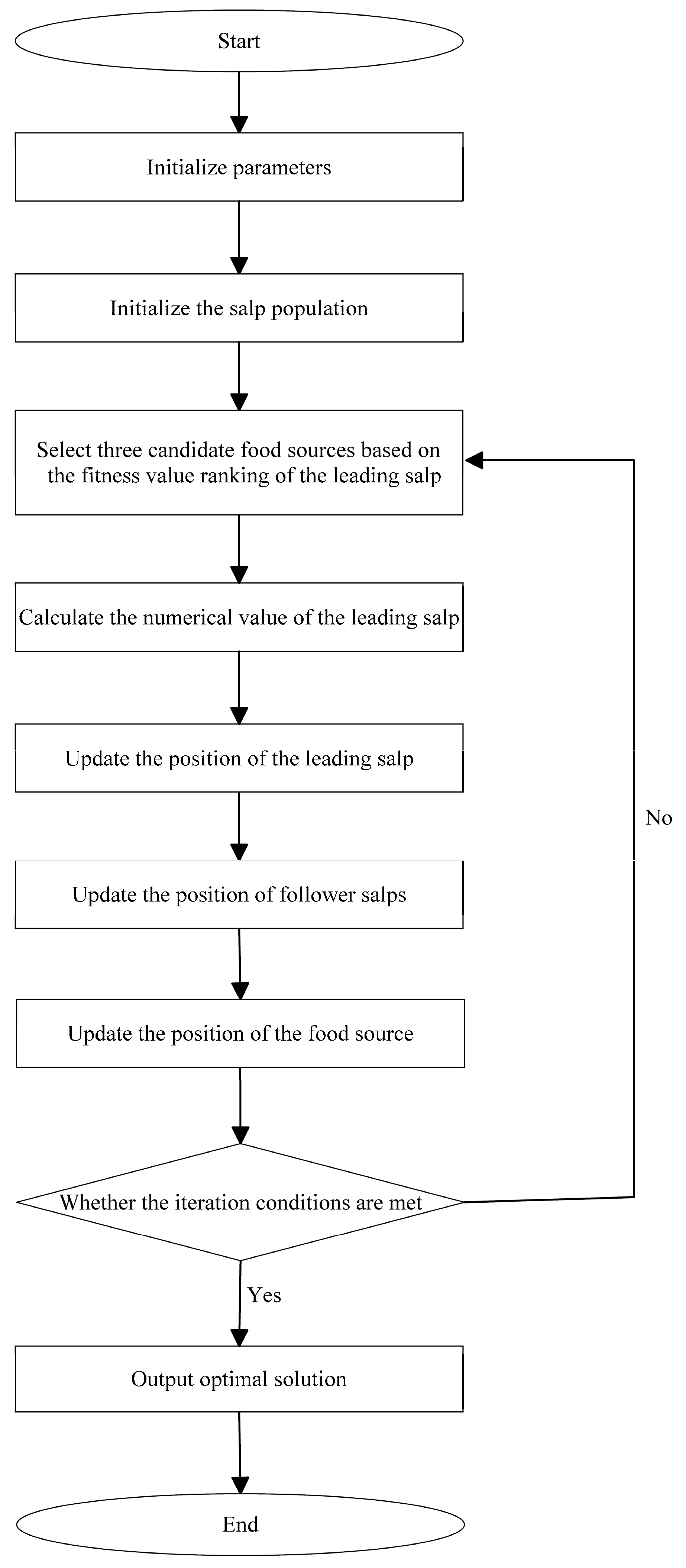
4. Improved Salp Swarm Algorithm

The optimization problem concerning the multi-temperature joint distribution route for fresh products is a complex combinatorial optimization challenge characterized by high dimensionality, multiple constraints, and non-linearity. In this paper, we employ the salp swarm algorithm (SSA), a metaheuristic optimization technique inspired by the biological behavior of salp swarms, as proposed by [34]. The traditional SSA offers several advantages, including a simple structure, minimal parameters, and ease of implementation. However, it also has notable drawbacks; specifically, it tends to converge prematurely to local optima and exhibits sensitivity to weight factors.

To enhance both the optimization performance and solving efficiency of the algorithm, we propose several improvements to the traditional SSA. The flowchart illustrating these enhancements is presented in Figure 1.

4.1. Adaptive Weight Factor

In the traditional SSA, the population is composed of a single leader and followers. The leader represents the individual positioned at the forefront of the salp chain, while the remaining individuals are classified as followers. This configuration leads to inadequate global search capabilities, a low proportion of leaders, and pronounced local search abilities throughout the algorithm’s iterative process. Consequently, this structure increases the likelihood of converging to local optima.

To address this problem, an adaptive weight factor method is proposed to modify the inertia weight in the SSA. This adjustment aims to balance the global and local search capabilities of the algorithm, thereby enhancing both its convergence speed and accuracy. The adaptive weight factor approach involves dynamically altering the magnitude of the inertia weight based on changes in fitness within the salp swarm population. Consequently, as iterations progress, there is a gradual reduction in the number of leader individuals while there is simultaneously an increase in the number of follower individuals.

This strategy allows for robust global search capability during the initial stages of iteration, which significantly improves convergence speed. In contrast, during later stages, emphasis shifts towards leveraging the local search abilities of followers to enhance optimization accuracy while still considering global search aspects within the algorithm.

The specific calculation method is as follows; let $r\times N$ represent the number of leaders in each generation of the population and $(1-r)\times N$ denote the number of followers. The formula for calculating the adaptive weight factor $r$ is presented below:

$$r=r_i-(r_i-r_f)\times \mathrm{t}\mathrm{a}\mathrm{n}({\displaystyle \frac{1}{\kappa }}\times {\displaystyle \frac{t}{T_{max}}}\times \pi ),$$

(22)

The notations used in the formula above are shown as follows:

${\mathrm{r}}_{\mathrm{i}}$: Control the initial value of $\mathrm{r}$;

${\mathrm{r}}_{\mathrm{f}}$: Control the final value of $\mathrm{r}$;

$\mathsf{\kappa }$: Nonlinear adjustment coefficient.

After conducting a substantial number of experiments, it was observed that the algorithm exhibits improved performance when ${\mathrm{r}}_{\mathrm{i}}$ is set to 0.7, ${\mathrm{r}}_{\mathrm{f}}$ is set to 0.3, and $\mathsf{\kappa }$ is set to 4.

4.2. Leader Position Update Strategy

The update of the leader position is a critical factor influencing the performance of the algorithm in SSA. In traditional SSA, this update is accomplished by randomly selecting a food source as the base target position and subsequently performing random perturbations around it to strike a balance between global and local search. However, this approach has several limitations.

Firstly, the randomly selected food source may not be optimal or even close to optimal, which can lead to an incorrect direction update for the leader’s position that deviates from the global optimum region. Secondly, both the amplitude and direction of these random disturbances are fixed and cannot be adaptively adjusted based on dynamic changes during the search process. This rigidity may result in step sizes that are either too large or too small, adversely affecting convergence speed and accuracy.

Moreover, updating leader positions solely relies on information from a single food source without fully leveraging data from other individuals within the population. This limitation reduces both information utilization and diversity.

To address the problem, an enhanced leader position update strategy based on the linear order crossover (LOX) technique is proposed. LOX is a crossover operation utilized in genetic algorithms to amalgamate the genetic information of two parent individuals into a new offspring. The fundamental principle of LOX involves representing the chromosomes of both parents as one-dimensional arrays, followed by cutting and exchanging segments at one or more randomly selected positions. This crossover operation preserves the sequence of genes within the central portion of each parent individual, thereby minimizing gene disruption and enhancing crossover effectiveness. Furthermore, employing the LOX strategy can augment individual diversity within the population, improve the algorithm’s exploratory capabilities, and mitigate the risk of convergence to local optima.

In addition, three individuals with the highest fitness levels are selected from the leadership group, denoted as $F_{\alpha }$, $F_{\beta }$, and $F_{\gamma }$, to serve as candidate food sources. The traditional SSA only selects the individual with the best fitness as the food source; this approach can easily lead to local optima. To mitigate this issue, this paper employs three candidate food sources to guide the remaining leaders in their search process. Based on the encoding method of the route optimization problem, the search mode is determined as follows:

$$F_j(t+1)=\left\{\begin{array}{l}LOX\left(F_j\right(t),F_{\alpha }(t\left)\right)\hspace{1em}\hspace{1em}rand<1/3\\ LOX\left(F_j\left(t\right),F_{\beta }\left(t\right)\right)\hspace{1em}1/3\le rand<2/3\\ LOX\left(F_j\right(t),F_{\gamma }(t\left)\right)\hspace{1em}\hspace{1em}otherwise\end{array}\right.,$$

(23)

The notations used in the formula above are shown as follows:

$F_j(t+1)$: The updated position of the th individual of the salp;

$F_{\alpha }$, $F_{\beta }$, $F_{\gamma }$: Alternative food sources.

In the process of updating the positions of individual leaders, salp individuals $F_{\alpha }$, $F_{\beta }$, and $F_{\gamma }$ with the top three fitness values in the leader group are initially selected. A random number $rand$ is then generated within the range of [0, 1]. Subsequently, based on different ranges of $rand$, other leader individuals from the current generation, excluding the three candidate food sources, are subjected to LOX operations with one of $F_{\alpha }$, $F_{\beta }$, and $F_{\gamma }$.

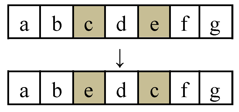
4.3. Follower Position Update Strategy

In traditional SSA, the update of follower positions is achieved by mimicking the feeding behavior of salps. Specifically, followers tend to follow the position of preceding salps in order to access better food sources. However, this reliance on the positions of previous salps for updating follower locations can lead to missed opportunities for discovering superior food sources, thereby diminishing search efficiency. Furthermore, a lack of diversity in updating follower positions may result in followers clustering around local optima, which further impairs their overall search capability.

Therefore, this paper employs equal probability to conduct single-point exchange, single-point insertion, and reversal operations on individual followers. The aforementioned strategies are grounded in chromosome-encoding mutation operators, which generate new positions by applying various operations to the elements of follower positions. This approach facilitates the enhancement of follower encoding both within and beyond local optima.

• Single-point exchange

Randomly select two positions within the coding sequence of a follower individual and exchange the codes at these selected positions. This single-point exchange operation can disrupt the original coding order, leading to new mutations, as illustrated in Figure 2.

2.

Single-point insertion

Randomly select a position of a follower individual and then insert the code at that position before the location of another randomly selected follower individual. Simultaneously, advance the code following its original position by one bit. This single-point insertion operation can alter the original encoding order, leading to new mutations, as illustrated in Figure 3.

3.

Reversal operations

Randomly select two positions within the encoding of a follower individual and then reverse the order of the elements between these two positions. This reversal operation preserves the original encoding while altering the relative arrangement of the selected elements, thereby introducing new mutations, as illustrated in Figure 4.

4.4. Gaussian Mutation Strategy for Food Source Location

In traditional SSA, the location of the food source is defined as the optimal individual within the salp swarm, which signifies the currently identified optimal solution. To enhance the diversity of food source locations and mitigate the risk of SSA converging to local optima, this paper incorporates a Gaussian mutation strategy for determining food source locations. The Gaussian mutation strategy is a widely utilized operation in metaheuristic algorithms that generates new solutions by adding a random number drawn from a Gaussian distribution to the original solution.

The Gaussian mutation strategy offers the advantage of dynamically adjusting the intensity of mutations based on the standard deviation parameter of the Gaussian distribution. This capability facilitates a balance between the algorithm’s global search efficiency and its local search effectiveness. The Gaussian mutation operator is employed to introduce random perturbations to the positions of the three candidate food sources $F_{\alpha }$, $F_{\beta }$, and $F_{\gamma }$, thereby facilitating a more comprehensive and effective search process. The detailed strategy for implementing Gaussian mutation is outlined as follows.

• Gaussian mutation strategy operation selection

The $2-swap$ operation employed in the Gaussian mutation strategy involves exchanging two dimensions of the original position vector. Specifically, this process entails randomly selecting two positions within the encoding sequence and subsequently rearranging the elements between these two positions in reverse order.

2.

Calculation of Gaussian mutation operation times

Perform $G$ mutation operations on candidate food sources $F_{\alpha }$, $F_{\beta }$, and $F_{\gamma }$, and the calculation formula for $G$ is as follows:

$$G=min(1,\lceil |e|\rceil ),$$

(24)

The notations used in the formula above are shown as follows:

$e\text{~}N\left(\mathrm{1,1}\right)$, $N\left(\mathrm{1,1}\right)$: A normal distribution with mean value and variance, respectively.

Therefore, a new solution can be derived that is similar to, yet not identical to, the original food source location; this represents the mutated food source position. Subsequently, the fitness of the mutated food source position is evaluated in comparison to that of the original food source position. If the fitness of the mutated food source position proves to be superior, it will replace the original food source position. Conversely, if it does not yield a higher fitness value, the original food source position will remain unchanged to ensure that there is no decline in fitness. Meanwhile, enhancing the diversity of food source positions is advantageous for enabling the algorithm to escape local optima and discover improved solutions.

4.5. The Pseudo Code of the Improved SSA

The pseudo code of the improved SSA is shown in Algorithm 1.

Algorithm 1. Improved SSA

1: Initialize population size N, Max iterations T_max, Temperature zones W, Vehicle capacity Q: Randomly generate N salp individuals (route plans) 2: while t ≤ T_max do 3:  Calculate fitness (total cost C) for each individual 4:  Select top 3 individuals as candidate food sources Fα, Fβ, Fγ 5:  Adaptively adjust weight factor r = 0.7 − 0.4 × tan(π × t/(4T_max)) // Equation (22) 6:  for each salp individual do 7:   if individual is leader (top r × N) then 8:    Perform LOX crossover with Fα/Fβ/Fγ via Equation (23) 9:   else // Followers 10:   Randomly apply single-point swap/insertion/reversal // Figure 2, Figure 3 and Figure 4 11:  end if 12:  Apply Gaussian mutation to Fα, Fβ, Fγ // Equation (24) 13:  end for 14:  Update global best solution X* 15:  t = t + 1 16: end while

5. Computational Experiments

5.1. Initial Setting

In order to assess the performance of the improved SSA introduced in Section 3, this paper utilized R110 data from the Solomon standard example as the test dataset. This dataset comprises a distribution center and 100 delivery points, each characterized by varying demands, time windows, and service times. Among these points, point number 0 is designated as the distribution center, while the X and Y coordinates of points numbered 1–30 are employed to represent the locations of each delivery point. The customer demand for each delivery node and temperature zone along with the required quantities of cold storage and insulation boxes, customer time windows, and service times are detailed in

Table 2. Information about delivery nodes.

No.	X	Y	F2 Temperature Zone	F1 Temperature Zone	C2 Temperature Zone	C1 Temperature Zone	Number of Cold Storage Boxes	Tei	tei	tli	Tli	Service Time
0	35	35	-	-	-	-	-	-	-	999	999	10
1	41	49	50	78	50	65	4	88	133	198	243	10
2	35	17	80	0	52	84	3	0	22	87	142	10
3	55	45	98	92	0	73	3	64	98	143	177	10
4	55	20	0	86	55	0	2	74	123	184	233	10
5	15	30	110	88	0	80	3	0	20	93	138	10
6	25	30	58	74	36	63	4	39	76	131	168	10
7	20	50	100	0	50	82	3	24	61	110	147	10
8	10	43	90	93	36	74	4	37	75	124	162	10
9	55	60	0	95	40	0	2	39	74	129	164	10
10	30	60	88	73	37	61	4	68	107	150	189	10
11	20	65	110	77	43	75	4	0	42	101	153	10
12	50	35	78	75	0	58	3	0	38	97	141	10
13	30	25	65	0	43	70	3	76	131	196	251	10
14	15	10	0	83	45	83	3	0	32	114	171	10
15	30	5	75	88	35	63	4	0	35	96	139	10
16	10	20	0	76	36	0	2	11	52	107	148	10
17	5	30	78	0	0	81	2	67	124	189	246	10
18	20	40	88	74	52	80	4	29	69	114	154	10
19	15	60	89	81	40	70	4	13	52	109	148	10
20	45	65	98	79	41	74	4	61	105	156	200	10
21	45	20	98	80	60	79	4	0	37	96	147	10
22	45	10	100	75	37	0	3	35	76	127	168	10
23	55	5	90	87	53	61	4	7	43	102	138	10
24	65	35	88	0	34	72	3	67	124	190	247	10
25	65	20	110	77	50	64	4	76	121	186	232	10
26	45	30	0	93	0	0	1	70	112	161	203	10
27	35	40	95	90	42	63	4	0	8	75	116	10
28	41	37	80	94	40	85	4	0	11	76	129	10
29	64	42	85	0	48	67	3	0	37	98	136	10
30	40	60	0	71	44	60	3	10	49	102	141	10

.

5.2. Parameter Settings

5.2.1. Model Parameter

The parameter settings in the proposed model are shown in

Table 3. Parameters in the proposed model.

Parameter	Value	Unit
$\mathrm{M}$	30	-
$\mathrm{W}$	4	-
${\mathrm{c}}_1$	80	CNY/vehicle
${\mathrm{c}}_2$	0.65	CNY/km
$\mathsf{\theta }$	2	CNY/product
${\mathsf{\delta }}_{\mathsf{\omega }}$	F2 temperature zone: 0.72 F1 temperature zone: 0.24 C2 temperature zone: 0.12 C1 temperature zone: 0	CNY
$\mathrm{v}$	60	km/h
${\mathrm{p}}_{\mathsf{\omega }}$	F2 temperature zone: 10 F1 temperature zone: 8 C2 temperature zone: 3 C1 temperature zone: 30	CNY/kg
${\mathrm{Q}}_{\mathsf{\omega }}$	F2 temperature zone: 110 F1 temperature zone: 95 C2 temperature zone: 60 C1 temperature zone: 85	kg
${\mathrm{r}}_{\mathsf{\omega }}$	F2 temperature zone: 0.02 F1 temperature zone: 0.05 C2 temperature zone: 0.05 C1 temperature zone: 0.02	-
${\mathsf{\epsilon }}_{\mathsf{\omega }}$	F2 temperature zone: 0.05 F1 temperature zone: 0.03 C2 temperature zone: 0.01 C1 temperature zone: 0.02	-
${\mathsf{\beta }}_{\mathrm{e}}$	1	CNY/min
${\mathsf{\beta }}_{\mathrm{l}}$	3	CNY/min
${\mathrm{P}}_{\mathrm{k}}$	20	-
$\mathrm{Q}$	1800	kg
${\mathsf{\xi }}_{\mathrm{m}}$	0.16	L/km
${\mathsf{\xi }}_0$	0.13	L/km
${\mathrm{e}}_{\mathrm{c}}$	0.226	kg/L
${\mathrm{C}}_{\mathrm{c}}$	0.02	CNY/kg

.

5.2.2. Algorithm Parameter

The algorithm proposed in this paper is implemented using Matlab R2022b. All experiments are conducted on a personal computer equipped with an Intel Core i7-7700HQ processor running at 2.8 GHz and 8 GB of RAM, under the Windows 10 operating system. The parameter settings for the algorithm are all based on the results of 30 preliminary experiments, shown in

Table 4. The algorithm parameter setting.

Parameter	Value
Initial population size	100
Maximum number of iterations	1000
Genetic algorithm crossover probability	0.8
Genetic algorithm mutation probability	0.5

.

5.3. Result Analysis

5.3.1. Small-Scale Experiment

To assess the feasibility of the model and algorithm proposed in this paper, we selected the first 10 delivery points of R110 from the Solomon standard calculation example for analysis in this section. The results are presented in Figure 5 and Figure 6, where Figure 5 illustrates the convergence behavior of the proposed algorithm, while Figure 6 depicts the delivery vehicle route. The total delivery cost is calculated to be CNY 966.32.

As illustrated in Figure 6, the small-scale experiment involved the utilization of two vehicles for the distribution of fresh products. The specific delivery routes are detailed in

Table 5. The detailed delivery route.

Vehicle	Delivery Route
1 (Yellow)	0 → 5 → 6 → 2 → 4 → 3 → 9 → 1 → 0
2 (Blue)	0 → 8 → 7 → 10 → 0

.

5.3.2. Performance Analysis of the Algorithm

In order to further validate the performance of the algorithm proposed in this paper, this section will compare the improved SSA with traditional SSA and genetic algorithm (GA). The results are presented in Figure 7 and Figure 8, while

Table 6. Comparison of total distribution cost of three algorithms in multi-temperature joint distribution mode.

	Improved SSA	Traditional SSA	Genetic Algorithm	GAP1	GAP2
Fixed cost (CNY)	400.00	480.00	560.00	16.7%	28.6%
Transportation cost (CNY)	398.61	420.49	539.82	5.2%	26.2%
Refrigeration cost (CNY)	222.04	222.04	222.04	0	0
Cargo damage cost (CNY)	2128.60	2159.37	2143.77	1.4%	0.7%
Penalty cost (CNY)	12.45	14.72	15.49	15.4%	19.6%
Carbon emission cost (CNY)	36.30	38.01	49.19	4.5%	26.2%
Total distribution cost (CNY)	3198.01	3334.63	3530.31	4.1%	9.4%

illustrates the cost comparison among the three algorithms under a multi-temperature joint distribution mode.

Note:

$${GAP}_1={\displaystyle \frac{\mathrm{R}\mathrm{e}\mathrm{s}\mathrm{u}\mathrm{l}\mathrm{t}\mathrm{s}\mathrm{o}\mathrm{f}\mathrm{t}\mathrm{r}\mathrm{a}\mathrm{d}\mathrm{i}\mathrm{t}\mathrm{i}\mathrm{o}\mathrm{n}\mathrm{a}\mathrm{l}\mathrm{S}\mathrm{S}\mathrm{A}-\mathrm{R}\mathrm{e}\mathrm{s}\mathrm{u}\mathrm{l}\mathrm{t}\mathrm{s}\mathrm{o}\mathrm{f}\mathrm{i}\mathrm{m}\mathrm{p}\mathrm{r}\mathrm{o}\mathrm{v}\mathrm{e}\mathrm{d}\mathrm{S}\mathrm{S}\mathrm{A}}{\mathrm{R}\mathrm{e}\mathrm{s}\mathrm{u}\mathrm{l}\mathrm{t}\mathrm{s}\mathrm{o}\mathrm{f}\mathrm{t}\mathrm{r}\mathrm{a}\mathrm{d}\mathrm{i}\mathrm{t}\mathrm{i}\mathrm{o}\mathrm{n}\mathrm{a}\mathrm{l}\mathrm{S}\mathrm{S}\mathrm{A}}}\times 100,$$

(25)

$${GAP}_2={\displaystyle \frac{\mathrm{R}\mathrm{e}\mathrm{s}\mathrm{u}\mathrm{l}\mathrm{t}\mathrm{s}\mathrm{o}\mathrm{f}\mathrm{G}\mathrm{A}-\mathrm{R}\mathrm{e}\mathrm{s}\mathrm{u}\mathrm{l}\mathrm{t}\mathrm{s}\mathrm{o}\mathrm{f}\mathrm{i}\mathrm{m}\mathrm{p}\mathrm{r}\mathrm{o}\mathrm{v}\mathrm{e}\mathrm{d}\mathrm{S}\mathrm{S}\mathrm{A}}{\mathrm{R}\mathrm{e}\mathrm{s}\mathrm{u}\mathrm{l}\mathrm{t}\mathrm{s}\mathrm{o}\mathrm{f}\mathrm{G}\mathrm{A}}}\times 100,$$

(26)

From Table 6, it is evident that the improved SSA outperforms both traditional SSA and GA in terms of fixed costs, transportation costs, penalty costs, carbon emission costs, and total distribution costs. This leads to a more effective reduction in overall logistics distribution expenses. Furthermore, as illustrated in Figure 7 and Figure 8, the optimization performance of the improved SSA is significantly superior to that of traditional SSA and GA; additionally, the resulting distribution routes are more compact and rationalized. This minimizes redundant driving distances while enhancing vehicle utilization efficiency.

Consequently, the improved SSA proposed in this paper not only demonstrates markedly better optimization capabilities compared to traditional SSA and GA but also effectively addresses the challenges associated with multi-temperature joint distribution route optimization for perishable products. Moreover, it leverages both collaborative and competitive dynamics between leaders and followers to elevate group intelligence levels. Simultaneously, the improved SSA exhibits greater adaptability to the specific characteristics and constraints inherent in route optimization problems, thereby enhancing solution quality and speed. Additionally, regarding complexity and uncertainty within path optimization issues, the refined SSA proves adept at overcoming these obstacles, thus significantly improving both the stability and reliability of solutions.

5.3.3. Comparative Experiment Between Different Distribution Modes

In order to assess the advantages of the multi-temperature joint distribution mode, a comparative experiment was conducted between this mode and the single product temperature distribution mode. The delivery vehicle route for the multi-temperature joint distribution mode is illustrated in Figure 8c and detailed in

Table 7. The detailed delivery route of the multi-temperature joint distribution mode.

Vehicle	Delivery Route
1 (Yellow)	0 → 20 → 9 → 29 → 3 → 12 → 0
2 (Blue)	0 → 27 → 15 → 16 → 4 → 25 → 24 → 0
3 (Green)	0 → 28 → 13 → 2 → 21 → 23 → 22 → 26 → 0
4 (Purple)	0 → 7 → 18 → 6 → 17 → 5 → 14 → 0
5 (Deep blue)	0 → 8 → 10 → 11 → 19 → 30 → 1 → 0

, whereas the delivery vehicle route for the single product temperature distribution mode is presented in Figure 9 and outlined in

Table 8. The detailed delivery route of the single product temperature distribution mode.

Vehicle	Delivery Route
C1 temperature zone 1 (Red)	0 → 6 → 5 → 17 → 0
C1 temperature zone 2 (Purple)	0 → 28 → 3 → 20 → 30 → 10 → 11 → 1 → 0
C1 temperature zone 3 (Deep blue)	0 → 27 → 13 → 2 → 21 → 23 → 25 → 0
C1 temperature zone 4 (Black)	0 → 18 → 7 → 19 → 8 → 0
C1 temperature zone 5 (Pink)	0 → 12 → 29 → 24 → 15 → 14 → 0
C2 temperature zone 1 (Pink)	0 → 27 → 28 → 1 → 30 → 20 → 9 → 0
C2 temperature zone 2 (Blue)	0 → 21 → 23 → 25 → 4 → 0
C2 temperature zone 3 (Green)	0 → 2 → 15 → 14 → 16 → 6 → 0
C2 temperature zone 4 (Yellow)	0 → 18 → 8 → 7 → 19 → 11 → 10 → 0
C2 temperature zone 5 (Deep yellow)	0 → 13 → 22 → 24 → 29 → 0
F1 temperature zone 1 (Black)	0 → 28 → 12 → 3 → 9 → 0
F1 temperature zone 2 (Deep green)	0 → 26 → 21 → 22 → 23 → 15 → 0
F1 temperature zone 3 (Light green)	0 → 10 → 11 → 19 → 8 → 5 → 16 → 14 → 0
F1 temperature zone 4 (Blue)	0 → 27 → 1 → 20 → 30 → 18 → 6 → 4 → 25 → 0
F2 temperature zone 1 (Red)	0 → 28 → 3 → 29 → 12 → 0
F2 temperature zone 2 (Black)	0 → 18 → 8 → 17 → 5 → 6 → 25 → 24 → 0
F2 temperature zone 3 (Light green)	0 → 27 → 7 → 19 → 11 → 10 → 20 → 1 → 0
F2 temperature zone 4 (Green)	0 → 21 → 22 → 23 → 15 → 2 → 13 → 0

. A cost comparison between these two modes is provided in

Table 9. Cost comparison between two modes.

	Fixed Cost (CNY)	Transportation Cost (CNY)	Refrigeration Cost (CNY)	Cargo Damage Cost (CNY)	Penalty Cost (CNY)	Carbon Emission Cost (CNY)	Total Distribution Cost (CNY)
Multi-temperature joint distribution mode	400.00	398.61	222.04	2128.60	12.45	36.30	3198.01
Single product temperature distribution mode	1440.00	1181.24	222.04	1682.70	16.17	107.79	4649.94
GAP3	72.2%	66.2%	0	−26.5%	23.0%	66.3%	31.2%

.

Note:

$${GAP}_3={\displaystyle \frac{\mathrm{C}\mathrm{o}\mathrm{s}\mathrm{t}\mathrm{o}\mathrm{f}\mathrm{s}\mathrm{i}\mathrm{n}\mathrm{g}\mathrm{l}\mathrm{e}\mathrm{p}\mathrm{r}\mathrm{o}\mathrm{d}\mathrm{u}\mathrm{c}\mathrm{t}\mathrm{t}\mathrm{e}\mathrm{m}\mathrm{p}\mathrm{e}\mathrm{r}\mathrm{a}\mathrm{t}\mathrm{u}\mathrm{r}\mathrm{e}\mathrm{d}\mathrm{i}\mathrm{s}\mathrm{t}\mathrm{r}\mathrm{i}\mathrm{b}\mathrm{u}\mathrm{t}\mathrm{i}\mathrm{o}\mathrm{n}\mathrm{m}\mathrm{o}\mathrm{d}\mathrm{e}-\mathrm{C}\mathrm{o}\mathrm{s}\mathrm{t}\mathrm{o}\mathrm{f}\mathrm{m}\mathrm{u}\mathrm{l}\mathrm{t}\mathrm{i}-\mathrm{t}\mathrm{e}\mathrm{m}\mathrm{p}\mathrm{e}\mathrm{r}\mathrm{a}\mathrm{t}\mathrm{u}\mathrm{r}\mathrm{e}\mathrm{j}\mathrm{o}\mathrm{i}\mathrm{n}\mathrm{t}\mathrm{d}\mathrm{i}\mathrm{s}\mathrm{t}\mathrm{r}\mathrm{i}\mathrm{b}\mathrm{u}\mathrm{t}\mathrm{i}\mathrm{o}\mathrm{n}\mathrm{m}\mathrm{o}\mathrm{d}\mathrm{e}}{\mathrm{C}\mathrm{o}\mathrm{s}\mathrm{t}\mathrm{o}\mathrm{f}\mathrm{s}\mathrm{i}\mathrm{n}\mathrm{g}\mathrm{l}\mathrm{e}\mathrm{p}\mathrm{r}\mathrm{o}\mathrm{d}\mathrm{u}\mathrm{c}\mathrm{t}\mathrm{t}\mathrm{e}\mathrm{m}\mathrm{p}\mathrm{e}\mathrm{r}\mathrm{a}\mathrm{t}\mathrm{u}\mathrm{r}\mathrm{e}\mathrm{d}\mathrm{i}\mathrm{s}\mathrm{t}\mathrm{r}\mathrm{i}\mathrm{b}\mathrm{u}\mathrm{t}\mathrm{i}\mathrm{o}\mathrm{n}\mathrm{m}\mathrm{o}\mathrm{d}\mathrm{e}}}\times 100,$$

(27)

According to Figure 8c and Figure 9, Table 8 and Table 9, it is evident that a total of five vehicles are required to complete the distribution of fresh products in the multi-temperature joint distribution mode. In contrast, 18 vehicles are necessary for the distribution of fresh products in the single product temperature distribution mode. This finding indicates that, within this experiment, the multi-temperature joint distribution mode achieves a reduction of 72.2% in vehicle resource utilization compared to the single product temperature distribution mode. Consequently, this approach effectively decreases the number of vehicles employed while enhancing the utilization rate of each vehicle.

Meanwhile, as illustrated in Table 9, while the multi-temperature joint distribution mode can reduce the number of delivery vehicles, it may also lead to an increase in transportation time for certain fresh products, consequently resulting in higher cargo damage costs. However, when compared to the traditional single-product temperature distribution mode, the multi-temperature joint distribution model has significantly decreased fixed costs, transportation costs, penalty costs, carbon emission costs, and total distribution costs by 72.2%, 66.2%, 23.0%, 66.3%, and 31.2%, respectively.

Additionally, in the multi-temperature joint distribution model, customers receive fresh products from various temperature zones during a single delivery process. The reduction in the number of delivery vehicles has led to substantial decreases in fixed costs, transportation costs, and carbon emissions, thus optimizing total distribution expenses considerably. Therefore, the multi-temperature joint distribution model presents significant advantages in terms of reducing logistics costs.

5.3.4. Analysis of Changes in Carbon Tax Prices

This paper examines the impact of carbon emission costs on the optimization of multi-temperature joint distribution routes for fresh products. It is posited that carbon emission costs are directly proportional to the carbon tax price. Consequently, fluctuations in carbon tax prices will influence the overall distribution cost associated with multi-temperature joint distribution of fresh products, thereby affecting both route selection and delivery vehicle arrangements.

To analyze how variations in carbon tax prices affect total distribution costs, this section considers five unit growth rates for carbon tax prices: 0%, 100%, 200%, 300%, and 400%. The corresponding total distribution costs and their respective growth rates are calculated. The results are presented in

Table 10. Results under different unit carbon tax prices.

Unit Carbon Tax Price (CNY/kg)	Unit Carbon Tax Price Growth Rate	Total Distribution Cost (CNY)	Growth Rate of Total Distribution Cost
0.02	0	3198.01	0
0.04	100%	3305.87	3.37%
0.06	200%	3412.71	3.23%
0.08	300%	3468.59	1.64%
0.1	400%	3520.49	1.50%

.

From Table 10, it is evident that the total distribution cost exhibits an upward trend as the unit carbon tax price increases. This phenomenon can be attributed to the fact that a rise in the unit carbon tax price elevates the carbon emission cost per unit of goods, consequently leading to an increase in the overall distribution cost. However, when the unit carbon tax price escalates from 0.06 CNY/kg to 0.08 CNY/kg, the growth rate of total distribution cost diminishes. This indicates that within this range, the influence of variations in the unit carbon tax price on total distribution cost gradually weakens.

It can be inferred that, while the unit carbon tax price is a significant influencing factor, its relationship with total distribution cost is not linear. Instead, there exists an inflection point at which the growth rate of total distribution cost reaches its maximum. Therefore, establishing a reasonable framework for setting unit carbon tax prices holds substantial guiding significance for logistics companies aiming to optimize their total distribution costs.

5.3.5. Analysis of Vehicle Load Changes

The variation in vehicle load will directly influence both the quantity and frequency of delivery vehicles utilized in the multi-temperature joint distribution of fresh products, consequently impacting the overall distribution cost. To ascertain a reasonable range for delivery vehicle loads and to provide valuable insights for decision-makers, this paper conducted five distinct experiments with vehicle loads set at 2000 kg, 1800 kg, 1600 kg, 1400 kg, and 1200 kg. The results are presented in

Table 11. Results under different vehicle loads.

Vehicle Load (kg)	The Number of Delivery Vehicles	Total Distribution Cost (CNY)
2000	5	3250.37
1800	5	3198.01
1600	6	3292.52
1400	6	3338.64
1200	7	3456.27

.

From Table 11, it is evident that when the vehicle load decreases from 2000 kg to 1800 kg, the number of delivery vehicles remains unchanged; however, the total distribution cost declines from CNY 3250.37 to CNY 3198.01. This reduction in vehicle load results in a decrease in the fixed costs associated with each vehicle, thereby enhancing the utilization rate of the fleet. As the vehicle load continues to diminish, both the number of delivery vehicles and total distribution costs exhibit an upward trend. This phenomenon occurs because a lower vehicle load reduces each vehicle’s loading capacity, which subsequently increases the demand for additional delivery vehicles and raises transportation and cargo damage costs.

Consequently, it can be concluded that vehicle load is a parameter exerting significant influence on model output results; however, its relationship is not strictly monotonic. Instead, there exists an approximate optimal value that minimizes both the number of delivery vehicles and total distribution costs.

6. Conclusions

This paper addresses the optimization problem associated with the distribution routes of fresh products within a multi-temperature joint distribution framework. Temperature zones are delineated based on the specific characteristics of fresh products, while also taking into account the actual constraints encountered during the distribution process. A mixed-integer programming model is formulated to minimize total distribution costs. To enhance the optimization performance of traditional SSA, various strategies are employed, including adaptive weight factors, LOX, single-point exchange, single-point insertion, reversal operations, and Gaussian mutation techniques. These adaptations aim to overcome limitations inherent in conventional SSA approaches.

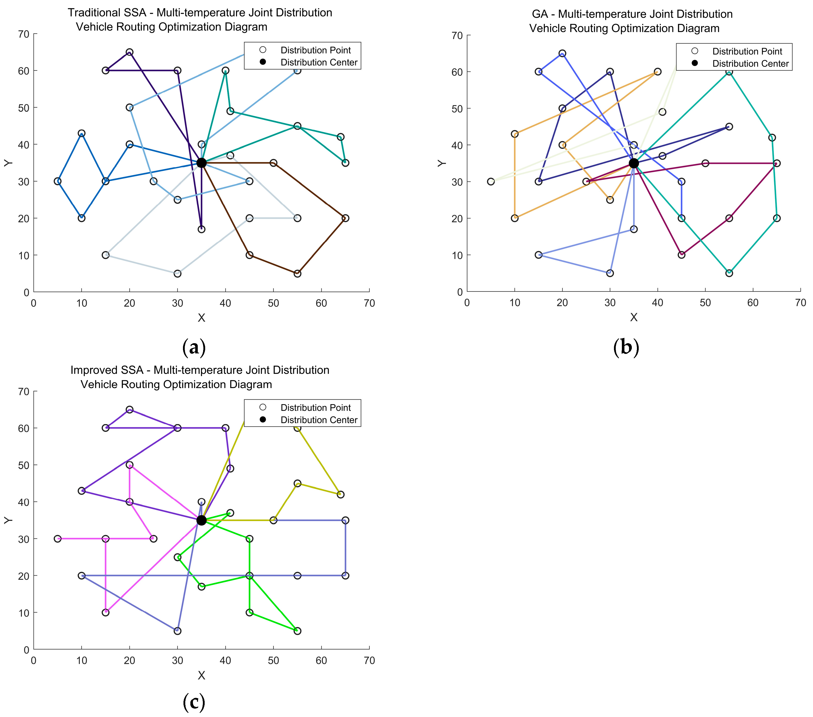
The data from R110 in the Solomon standard calculation example were utilized for five groups of computational experiments. Firstly, the initial ten delivery points were selected for analysis to verify the feasibility of the proposed model and algorithm. Subsequently, four large-scale comparative experiments were conducted. The results indicated that, although the cargo damage cost increased by 26.5% under the multi-temperature joint distribution mode compared to the single product temperature distribution mode, there was a significant reduction in fixed costs (72.2%), transportation costs (66.2%), penalty costs (23.0%), carbon emission costs (66.3%), and total distribution costs (31.2%). Additionally, the utilization rate of distribution vehicles improved.

Furthermore, as unit carbon tax prices increase, total distribution costs also rise; however, the growth rate of these costs gradually decreases over time. Conversely, as vehicle load diminishes, total distribution costs continue to escalate after reaching an inflection point. Moreover, when compared with traditional SSA and genetic algorithms, the improved SSA demonstrates superior optimization performance and cost efficiency in addressing such problems effectively.

Future research should consider the incorporation of dynamic location information and the development of a dynamic route optimization model. This approach would enable distribution plans to be adjusted and updated in response to real-time changes in location. Additionally, it is crucial to conduct comparisons with other state-of-the-art metaheuristics currently available in the field. Furthermore, it is essential to explore additional mutation strategies and encoding operations, as well as more effective methods for parameter selection, to enhance the algorithm’s problem-solving capabilities and adaptability in future applications.