Article

Mining High-Efficiency Itemsets with Negative Utilities

Department of Computer Engineering, Faculty of Engineering and Architecture, Erzurum Technical University, 25050 Erzurum, Türkiye
Mathematics 2025, 13(4), 659; https://doi.org/10.3390/math13040659
Submission received: 3 January 2025 / Revised: 26 January 2025 / Accepted: 6 February 2025 / Published: 17 February 2025
(This article belongs to the Section E1: Mathematics and Computer Science)

Abstract

:
High-efficiency itemset mining has recently emerged as a new problem in itemset mining. An itemset is classified as a high-efficiency itemset if its utility-to-investment ratio meets or exceeds a specified efficiency threshold. The goal is to discover all high-efficiency itemsets in a given database. However, solving the problem is computationally complex, due to the large search space involved. To effectively address this problem, several algorithms have been proposed that assume that databases contain only positive utilities. However, real-world databases often contain negative utilities. When the existing algorithms are applied to such databases, they fail to discover the complete set of itemsets, due to their limitations in handling negative utilities. This study proposes a novel algorithm, MHEINU (mining high-efficiency itemset with negative utilities), designed to correctly mine a complete set of high-efficiency itemsets from databases that also contain negative utilities. MHEINU introduces two upper-bounds to efficiently and safely reduce the search space. Additionally, it features a list-based data structure to streamline the mining process and minimize costly database scans. Experimental results on various datasets containing negative utilities showed that MHEINU effectively discovered the complete set of high-efficiency itemsets, performing well in terms of runtime, number of join operations, and memory usage. Additionally, MHEINU demonstrated good scalability, making it suitable for large-scale datasets.

1. Introduction

Frequent itemset mining (FIM) [1,2,3,4,5,6,7] is a popular data mining technique for identifying frequently occurring itemsets in transactional databases. However, FIM assumes that all items have equal importance and that each item may appear only once per transaction, which does not reflect real-world scenarios, where items have varying significance and quantities. For example, in retail, frequently purchased items may yield a low profit, while less frequent ones could be more profitable. As FIM focuses solely on item frequency, it may overlook itemsets that are less common but more valuable, making its results less meaningful or inadequate for decision-making processes.
To overcome this limitation, the problem of high-utility itemset mining (HUIM) [8] has been introduced. Unlike FIM, which targets frequent itemsets, HUIM identifies itemsets with high utility, considering factors like utility, profit, importance, weight, or other user-defined metrics. HUIM typically considers the internal utility (e.g., quantity sold) of items in transactions and the external utility (e.g., profit per unit) of items. The utility of an item in a transaction is derived by multiplying its external utility by its internal utility in that transaction. The utility of an itemset in a database is defined as the sum of the utilities of all items within the itemset across the transactions in which the itemset appears. The HUIM problem has attracted considerable attention from researchers, leading to the development of various algorithms [9,10,11,12,13,14,15,16,17,18,19,20,21,22] to effectively solve the problem.
However, while HUIM addresses the shortcomings of FIM by identifying high-utility itemsets, it overlooks another crucial factor: investment, which involves allocating resources to achieve potential future benefits [23,24]. Thus, HUIM may not fully support decision-makers aiming to maximize profits, because it does not account for the capital required to acquire products before selling them [23]. For example, consider two itemsets, X (a smartphone and a smartwatch) and Y (a monitor and a keyboard), with utilities of $400 and $100, respectively. Based on these figures alone, HUIM suggests that X is more significant than Y for making profits. However, if the investments in X and Y are $1000 and $200, respectively, the utility-to-investment ratio for X is 0.4 (400/1000), while for Y it is 0.5 (100/200). This means that when planning to maximize future profits, it is more advantageous to invest in Y rather than X. This is because, with the same capital of $100,000, a businessman can buy 100 units of X and earn a profit of $40,000. However, if the businessman chooses to invest in Y instead, he would be able to buy 500 units and earn a profit of $50,000. This demonstrates that a higher investment-to-utility ratio can provide better returns, even when the total utility of an itemset is lower [24].
To address this limitation of HUIM, the problem of high-efficiency itemset mining (HEIM) [23] was recently introduced, which considers both utility and investment. The efficiency of an itemset is calculated by dividing its utility by its investment. If this efficiency meets or exceeds a given minimum efficiency threshold ( m i n E ), the itemset is classified as a high-efficiency itemset ( H E I ). The goal of HEIM is to discover the complete and correct set of H E I s for a given m i n E within a dataset. However, solving the HEIM problem is a computationally complex task because of its large search space. Moreover, the efficiency values of itemsets cannot be used to prune the search space because the efficiency metric lacks monotonic or anti-monotonic properties [24]. In other words, for any itemset X and its superset X , the efficiency of X is not guaranteed to be less than or equal to the efficiency of X , which means the efficiency metric does not exhibit the monotonic property. Similarly, the efficiency of X is not guaranteed to be greater than or equal to the efficiency of X , meaning it does not follow the anti-monotonic property.
HEPM [23], the first algorithm proposed for the HEIM problem, introduced an efficiency upper-bound ( e u b ) to overcome this challenge. This upper-bound guarantees the anti-monotonic property by overestimating the efficiency values of the itemsets and helps to prune the search space. Although e u b is useful for this purpose, HEPM generates many candidates and requires multiple database scans [23]. To further improve the mining process for the HEIM problem, the HEPMiner [23] and MHEI [24] algorithms were developed. HEPMiner uses a list-based data structure, while MHEI employs a database projection and merging method. Both use their own upper-bounds, along with e u b for further pruning of the search space. Among them, MHEI has demonstrated the best performance [24].
However, as noted in various studies [25,26], real-world databases often include items with negative utilities. For instance, large supermarket chains frequently run bundled or cross-promotion campaigns where some items are sold at a loss (negative utility to boost overall profits by increasing sales of related products) [25,27]. This strategy is not confined to retail but is widely observed across other sectors [28]. In the telecommunications industry, companies often offer discounted or bundled services that initially result in a loss but are designed to attract new customers or retain existing ones. For instance, discounted mobile phone plans bundled with data packages are commonly used to secure long-term profitability through upselling or cross-selling additional services. Similarly, in the hospitality sector, negative utility frequently occurs in bundled offerings. Hotels, for example, may offer discounted accommodation rates paired with ancillary services such as dining, spa, or recreational activity packages. While the accommodation itself may incur a loss, the overall revenue is enhanced through the additional services. The software industry adopts similar strategies by offering heavily discounted subscription packages for bundled services. Although these bundles may generate an immediate loss (negative utility), they help foster customer retention and generate a foundation for recurring revenue. Moreover, negative-utility-based mining extends its applicability beyond retail areas and cross-selling strategies to various domains, including website clickstream data, biomedical applications, and mobile commerce [29,30]. Additionally, in the investment sector, particularly in stock portfolio management, negative utility can be leveraged to optimize returns by accounting for the daily losses of stocks. For example, in [31], a data mining framework was developed to help investors plan and manage diversified stock portfolios for long-term investments. By analyzing historical stock data and incorporating negative utility, the designed approach enables the optimization of portfolio strategies, leading to improved overall performance.
On the other hand, the existing HEIM algorithms were developed based on the assumption that the datasets contain only positive utilities. Therefore, when applied to such databases, they do not guarantee the discovery of the complete set of H E I s . The reason for this is that the existing algorithms prune the search space based on upper-bounds, which overestimate the efficiency of itemsets by considering all the items as having positive utilities. When a database contains items with negative utilities, these overestimations can turn into underestimations, causing incorrect pruning of itemsets that are actually H E I s . As a result, since the existing HEIM algorithms fail to discover the complete set of H E I s for datasets with negative utilities, they are insufficient for providing decision-makers with the necessary information. Therefore, it is crucial to develop methods that can effectively address this issue.
This study addresses a significant gap in existing HEIM algorithms, which fail to fully discover H E I s from datasets with negative utilities. To tackle this challenge, the study developed methods and techniques for the efficient and complete discovery of H E I s from such databases. The key contributions of this paper are as follows:
-
Two novel upper-bounds, along with pruning strategies, are introduced to efficiently and safely prune the search space. These upper-bounds are designed to ensure that H E I s are not mistakenly pruned in the presence of negative utilities and to increase mining efficiency by early detection of itemsets that are not H E I s .
-
A list-based data structure, E L N U (efficiency-list with negative utilities), is proposed to store essential information for mining H E I s from databases with negative utilities. This structure minimizes the need for costly database scans, making the mining process more efficient.
-
An algorithm named MHEINU (mining high-efficiency itemset with negative utilities) is proposed to extract a correct and complete set of H E I s from databases with negative utilities, under a user-defined minimum efficiency threshold.
-
Comprehensive experiments were conducted on a variety of datasets with differing characteristics. The results validated the efficiency and effectiveness of the MHEINU algorithm for mining H E I s in databases with negative utilities, evaluating factors such as runtime, number of join operations, memory consumption, scalability, and the number of discovered itemsets.
The rest of the paper is structured as follows. Section 2 covers the related work. Section 3 outlines the fundamental concepts of the HEIM problem and discusses the problem faced by existing methods when dealing with databases containing negative utilities. Section 4 introduces the upper-bounds and the data structure, and explains the mining procedure of the proposed MHEINU algorithm. Section 5 provides the experimental results. Section 6 discusses some limitations of the HEIM problem. Finally, Section 7 concludes the paper and suggests directions for future research.

2. Related Work

High-utility itemset mining (HUIM) [8] aims to discover itemsets with high utility values in databases. The development of various algorithms has enhanced the efficiency of solving HUIM, starting with the two-phase algorithm [8]. This algorithm generates candidate itemsets in the first phase and identifies high-utility itemsets in the second phase, requiring multiple database scans, making it time-consuming. Subsequent algorithms, such as UP-Growth and UP-Growth+ [9], were introduced to reduce the number of database scans and candidates generated by utilizing their own techniques. However, they still struggle with the computational complexity of candidate generation processes. To address the challenges of candidate generation, single-phase algorithms like HUI-Miner [10], FHM [11], d2HUP [12], HUP-Miner [13], EFIM [14], IMHUP [15], mHUIMiner [16], HMiner [17], UPB-Miner [18], iMEFIM [19], and Hamm [20] were developed. These algorithms minimize database scans using tailored data structures or techniques such as database projection and merging. They significantly improve the HUIM process by reducing the search space with effective pruning strategies. Beyond classical algorithms, specialized methods have been developed for various HUIM extensions to address real-world application needs, such as mining closed H U I s  [32], sequential H U I s  [33], top-k H U I s  [34,35], correlated H U I s  [36], itemsets ignoring internal utilities [37], high average-utility itemsets [38,39], high-utility occupancy itemsets [40,41], significant utility discriminative itemsets [42], and solving HUIM in incremental [43,44] or time-stamped data [45], and so on.
However, none of the abovementioned studies considered the investment associated with itemsets during the mining process. As a result, while they identified itemsets with high utilities, they failed to reflect the true efficiency of these itemsets. This oversight limits decision-making for maximizing profit, as it disregards the investment values of the itemsets.
To address this limitation, the problem of high-efficiency itemset mining (HEIM) [23] was recently introduced, considering both utility and investment. According to HEIM, the importance of an itemset is determined by dividing its utility by its investment, defining this ratio as efficiency. HEIM aims to find all itemsets whose efficiency meets a user-defined threshold. However, due to the nature of the efficiency calculation, the efficiency measure does not exhibit monotonic or anti-monotonic properties. In other words, the efficiency values of the itemsets do not allow predicting in advance whether their supersets (or subsets) will be efficient, which complicates the problem computationally, due to the large search space. The first solution to this problem, the HEPM [23] algorithm, introduced an upper-bound called an efficiency upper-bound ( e u b ), which overestimates the efficiency values of itemsets to satisfy anti-monotonicity, aiding in pruning the search space. HEPM uses a level-based candidate generation and testing strategy, conducting multiple database scans to generate candidates and filter them by calculating their actual efficiency, making it time-consuming due to the extensive number of scans and candidates. The working principle of HEPM is as follows. It employs a two-phased approach to identify H E I s in a dataset. In Phase 1, the algorithm explores the search space using a breadth-first search strategy. It begins by scanning the dataset to collect the e u b values for each item. Items whose e u b values meet a given m i n E 
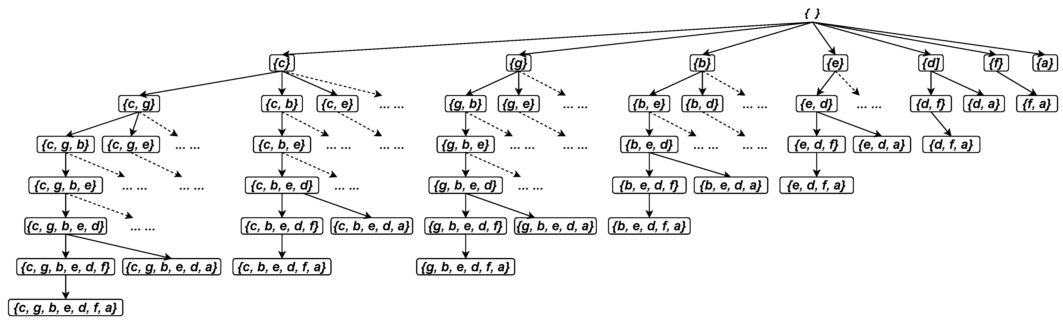
threshold are identified as candidate 1-itemsets. Subsequently, the algorithm iteratively generates candidate 2-itemsets from 1-itemsets, candidate 3-itemsets from 2-itemsets, and so on, continuing until no new candidates can be generated. In each iteration, the algorithm produces candidate (k + 1)-itemsets based on the current k-itemsets. A new (k + 1)-itemset is formed by appending the last item of one k-itemset to another k-itemset, provided they share the same (k − 1) items. During the examination of the search space, the newly generated candidates are filtered based on their e u b values. The final result of Phase 1 is the complete set of candidate itemsets. In Phase 2, the algorithm scans the database for each candidate itemset to calculate its actual efficiency. Itemsets having efficiencies that meet the m i n E threshold are returned as H E I s , which constitute the final output.
To overcome the issues seen in HEPM, the HEPMiner [23] algorithm was developed, utilizing a compact-list structure called an efficiency-list ( E L ). The E L of items stores the necessary information to mine H E I s . The E L of a k-itemset, where k ≥ 2, is constructed by joining the E L s of two ( k 1 ) -itemsets that share the same prefix itemset. HEPMiner further prunes the search space using additional upper-bounds, such as s e u b and s e u b w , alongside a matrix called an estimated efficiency co-occurrence structure ( E E C S ) for storing e u b values of each 2-itemset. The working principle of HEPMiner is as follows. First, it calculates the e u b of each item by scanning the database once. Then, it compares the e u b value of each item with a given m i n E threshold. In the second database scan, it disregards the items that do not meet the threshold and sorts the remaining items in each transaction alphabetically. During this process, it generates an E L list for each remaining item and an E E C S structure to store the e u b values of 2-itemsets. Afterward, the algorithm starts exploring the search space. For each itemset it visits in the search space, it first checks whether it is a H E I . Then, it calculates the s e u b value of the itemset and decides whether the extensions should be pruned. If the extensions are to be explored, it constructs E L lists for all 1-item extensions of the itemset. It discards the extensions with a s e u b w value lower than m i n E . It also decides whether E L lists need to be constructed for itemsets based on the corresponding value stored in the E E C S structure. The algorithm then continues exploring the search space recursively using a depth-first search strategy, along with the newly constructed E L lists. Using the values stored in the E L lists, the algorithm can easily calculate the efficiency of the itemsets, s e u b and s e u b w . For more details on the s e u b , s e u b w , E L , and E E C S structures and their construction, please refer to the original paper [23]. Although HEPMiner is more efficient than HEPM, it suffers from costly join operations required during the construction of lists. Subsequently, the MHEI [24] algorithm was introduced, employing a depth-first search with horizontal database representation. MHEI reduces database scanning costs through database projection and transaction merging, storing transaction identifiers for each item in the projected databases. It also introduced four upper-bounds, called sub-tree efficiency ( s e f ), stricter sub-tree efficiency ( s s e f ), local efficiency ( l e f ), and stricter local efficiency ( s l e f ), to enhance pruning effectiveness. The MHEI algorithm operates as follows. First, it performs a database scan to calculate the e u b values for each item and eliminates items whose e u b values do not meet the m i n E threshold, as in HEPMiner. The remaining promising items are then sorted based on a predefined order. During the second database scan, the algorithm considers only the promising items and reorganizes transactions according to the specified order of the items. If any transaction becomes empty after removing unpromising items, it is removed from the database. The rearranged transactions are then subjected to a sorting process to keep similar transactions close to each other. This facilitates the merging of identical projected transactions in later steps. The algorithm then scans the reorganized database, calculating the s s e f values for each item and storing the IDs of the transactions it finds in a list called C I D . Accordingly, items whose s s e f values do not satisfy the m i n E threshold are eliminated. Following this, MHEI performs a depth-first search to explore the search space. This is an iterative process where a prefix itemset, X (initially an empty set), is extended by adding a single item and evaluating the potential for further extensions. For each single-item extension of X with an item i, denoted as Z = { X i } , the projected database of X is scanned to compute the efficiency value of Z and obtain its projected dataset. If the efficiency value of Z satisfies the m i n E threshold, Z is identified as a H E I . Subsequently, for the per item v that follows i in the processing order, the values s s e f ( X , v ) and s l e f ( X , v ) , as well as the C I D of v within the projected database of Z, are obtained. Any item (along with Z) whose s s e f value satisfies m i n E is considered a potential single-item extension of Z, while items with s l e f values satisfying m i n E are considered for future extensions of Z. Extensions with s s e f and s l e f values below m i n E are discarded. The new prefix becomes Z, and the same process is repeated until the exploration procedure terminates. Note that, to reduce database scanning costs, the algorithm applies a transaction merging step to each projected database. Additionally, the C I D of itemsets is only used to examine the required transactions, which provides further time savings. For detailed information on the calculation of upper-bounds, transaction merging, and database projection, please refer to the original paper [24]. MHEI outperforms both HEPM and HEPMiner in runtime, memory consumption, and the number of generated candidates [24]. Additionally, the HEIM problem has been extended to the high-average-efficiency itemset mining (HAEIM) problem, which more fairly evaluates the efficiency of itemsets of different lengths [46]. In HAEIM, the importance of itemsets is determined using a metric called average-efficiency. The average-efficiency of an itemset is calculated by dividing its efficiency by its length (the number of items in the itemset).
However, all existing HEIM algorithms assume that databases contain only positive utilities, leading to incomplete discovery of H E I s when applied to databases that also contain negative utilities. The primary reason for this is that the upper-bound models used by existing algorithms may underestimate the actual efficiency values of itemsets in the presence of negative utilities. This causes the search space to be pruned incorrectly, missing important H E I s , and provides decision-makers with incomplete insights, which can hinder their ability to make informed decisions. To address this limitation, this study focuses on developing techniques for the complete and correct discovery of H E I s in databases that contain both positive and negative utilities. This ensures that decision-makers are provided with comprehensive and reliable data, allowing them to optimize future strategies based on a full understanding of past behaviors. This is especially valuable in real-world applications, where negative utility can represent costs or losses, as seen in retail promotions, bundled services, or investment strategies.

3. Preliminaries and Problem Statement

This section covers the basic concepts of HEIM problem. It also discusses the limitations the existing HEIM algorithms face when they are applied to databases with negative utility values.
Consider a set of items I = { i 1 , i 2 , , i n } , where each item has an external utility e u ( i ) and a unit investment value u I n v ( i ) . A transactional database D B is defined as a collection of transactions: D B = { T 1 , T 2 , , T m } . Each transaction T j in D B can contain any subset of the items in I, and for each item i in T j , there is an internal utility i u ( i , T j ) .
For example, consider the sample database D B shown in Table 1. It consists of eight transactions and contains the set of items I = { a , b , c , d , e , f , g } . For example, in the first transaction, T 1 , the items a, c, d, and f appear with internal utilities of 5, 4, 1, and 2, respectively. Thus, i u ( a , T 1 ) = 5 i u ( c , T 1 ) = 4, i u ( d , T 1 ) = 1, and i u ( f , T 1 ) = 2. The external utility and unit investment values of the items are provided in Table 2. For example, the external utility of item a is e u ( a ) = 1, and its unit investment is u I n v ( a ) = 2.
The external utility of an item can be either positive or negative. As shown in Table 2, items a, b, d, and g have positive external utilities, while the remaining items have negative external utilities. Note that the terms “positive items” and “negative items” will be used to denote items with positive and negative external utilities, respectively, throughout this paper.
Definition 1
(Total investment [23]). The total investment of an item i in a given database D B , denoted as i n v ( i ) , is defined as
i n v ( i ) = u I n v ( i ) × i T j T j D B i u ( i , T j ) .
The total investment of an itemset X in a given database D B , denoted as i n v ( i ) , is defined as
i n v ( X ) = i k X i n v ( i k ) .
For example, item a appears in transactions T 1 , T 3 , T 5 , and T 8 . Therefore, the total investment of item a, i n v ( a ) , is calculated as i n v ( a ) = u I n v ( a ) × ( i u ( a , T 1 ) + i u ( a , T 3 ) + i u ( a , T 5 ) + i u ( a , T 8 ) ) = 2 × (5 + 3 + 2 + 2) = 24. The total investment value of each item is given in Table 3. As another example, the total investment of the itemset { a , d , f } is calculated as i n v ( { a , d , f } ) = i n v ( a ) + i n v ( d ) + i n v ( f ) = 24 + 50 + 28 = 102.
Definition 2
(Utility [14]). The utility of an itemset X in a given transaction T j , where X ⊆ T j , denoted as u ( X , T j ) , is defined as
u ( X , T j ) = i k X i u ( i k , T j ) × e u ( i k ) .
The utility of an itemset X in a given database D B , denoted as u ( X ) , is defined as
u ( X ) = X T j T j D B u ( X , T j ) .
For example, consider the itemset { a , d , f } , which appears in transactions T 1 , T 3 , T 5 , and T 8 . The utility of { a , d , f } in T 1 is calculated as u ( { a , d , f } , T 1 ) = i u ( a , T 1 ) × e u ( a ) + i u ( d , T 1 ) × e u ( d ) + i u ( f , T 1 ) × e u ( f ) = 5 × 1 + 1 × 5 + 2 × (−1) = 8. Similarly, the utilities of { a , d , f } in transactions T 3 , T 5 , and T 8 are obtained as 22, 15, and 8, respectively. Consequently, the utility of { a , d , f } in the database D B is u ( { a , d , f } ) = 8 + 22 + 15 + 11 = 56.
Definition 3
(Efficiency of an itemset [23]). The efficiency of an itemset X in a given database D B , denoted as e ( X ) , is defined as
e ( X ) = u ( X ) / i n v ( X ) .
For example, the efficiency of the itemset { a , d , f } is calculated as e ( { a , d , f } ) = 56/102 = 0.5490.
Definition 4
(High-efficiency itemset [23]). An itemset X is classified as a high-efficiency itemset ( H E I ) if its efficiency is not lower than a specified minimum efficiency threshold ( m i n E ).
For example, if m i n E is set to 0.35, then the itemset { a , d , f } is a H E I , since e ( { a , d , f } ) = 0.5490 ≥ m i n E = 0.35. Table 4 summarizes all the itemsets that are H E I s within the sample D B presented in Table 1, when m i n E = 0.35.
However, solving the HEIM problem is challenging and complex, due to its large search space. Furthermore, the efficiency of itemsets cannot be used to reduce the search space, since the efficiency measure does not have an anti-monotonic (or monotonic) property. To address this, researchers [23,24] have focused on developing upper-bounds that overestimate the efficiency values of itemsets, providing the anti-monotonic property needed to effectively prune the search space. On the other hand, the existing upper-bounds were developed under the assumption that databases contain only positive items. When databases also include negative items, these upper-bounds may underestimate the efficiency of itemsets, leading to incorrect pruning of the search space. Consequently, applying the existing HEIM algorithms to databases with negative items may result in incomplete discovery of H E I s . To better understand this issue, let us consider one of the existing upper-bounds, called the efficiency upper-bound ( e u b ) [23], which is utilized by all existing HEIM algorithms to prune the search space. The details of the e u b model are as follows.
Definition 5
(Efficiency upper-bound (eub) [23]). Let the transaction utility ( t u ) of a transaction T j be defined as the sum of the utility values of all items within that transaction, given by
t u ( T j ) = i k T j u ( i k , T j ) .
Let the transaction weighted utility ( t w u ) of an itemset X be the sum of the t u values of all transactions that contain X, defined as
t w u ( X ) = X T j T j D B t u ( T j ) .
The efficiency upper-bound of X is defined as the ratio of the t w u to the total investment of X, and it is given by
e u b ( X ) = t w u ( X ) / i n v ( X ) .
Based on the anti-monotonic property of e u b , for any itemset X and its supersets X , the inequality e ( X ) e u b ( X ) e u b ( X ) holds [23]. This implies that e u b ( X ) serves as an overestimation of the efficiency of X and its supersets. Accordingly, X or any of its supersets cannot be a H E I if e u b ( X ) < m i n E , and, therefore, they can be pruned from the search space without further examination.
However, in databases with negative items, the anti-monotonic property of e u b may no longer hold. In other words, for any itemset X, e u b ( X ) might underestimate the efficiency of X or any of its supersets. For example, let us consider the itemset { a , d , f } . This itemset appears in transactions T 1 , T 3 , T 5 , and T 8 . The transaction utility of T 1 is calculated as t u ( T 1 ) = u ( a , T 1 ) + u ( c , T 1 ) + u ( d , T 1 ) + u ( f , T 1 ) = 5 × 1 + 4 × (−3) + 1 × 5 + 2 × (−1) = −4. For the other transactions, t u ( T 3 ) = 4, t u ( T 5 ) = 13, and t u ( T 8 ) = 11. Thus, t w u ( { a , d , f } ) = t u ( T 1 ) + t u ( T 3 ) + t u ( T 5 ) = 14 + t u ( T 8 ) = −4 + 4 + 13 + 11 = 24. Consequently, e u b ( { a , d , f } ) = t w u ( { a , d , f } ) / i n v ( { a , d , f } ) = 24/102 = 0.2353. Accordingly, itemset { a , d , f } or any of its supersets cannot be classified as a H E I when M i n E = 0.35 and can thus be pruned based on e u b ( { a , d , f } ) = 0.2353. However, e ( { a , d , f } ) = 0.5490 ≥ 0.35, so itemset { a , d , f } is a H E I . As another example, consider the item b. e u b ( b ) = ( t w u ( b ) = ( t u ( T 2 ) + t u ( T 6 ) )/ i n v ( b ) = (0 + (−6))/9 = −0.6667. In this case, no matter how low m i n E is, item b or any of its supersets can never be classified as a H E I according to the e u b ( b ) . However, item b is also a H E I when m i n E = 0.35.

4. Mining High-Efficiency Itemsets with Negative Utilities

This study introduces an algorithm named MHEINU (mining high-efficiency itemsets with negative utilities), specifically designed to extract H E I s from databases also containing negative utilities. The algorithm employs two upper-bounds, each integrated with an effective pruning strategy, and utilizes a list-based data structure to enhance performance.
The first part of this section introduces two new upper-bounds to safely reduce the search space of the HEIM problem with negative utilities. The next subsection describes a list-based data structure called E L N U (efficiency-list with negative utilities), which stores the information necessary for extracting H E I s . The subsequent subsection discusses the set-enumeration tree of the search space of the problem. The following subsection outlines the overall process of the proposed MHEINU algorithm, including its pseudo-code. The next subsection addresses the correctness and completeness of the proposed MHEINU algorithm. Finally, the last subsection provides an execution trace of the algorithm using an illustrative example.

4.1. Proposed Upper-Bounds

This study introduces two upper-bounds, along with corresponding pruning strategies, to efficiently and safely reduce the search space, thereby enhancing the mining process of the HEIM problem with negative utilities.
The first upper-bound, called the upper-bound efficiency with negative utilities ( u b e n ), is designed to determine whether an itemset and its supersets can contain any H E I s . Details are provided below.
Definition 6
(Positive utility of a transaction). The positive utility of a transaction T j , denoted as p u ( T j ) , is defined as
p u ( T j ) = i k T j e u ( i k ) 0 u ( i k , T j ) .
For example, consider transaction T 1 . It contains two positive items, a and d. The positive utility of T 1 is calculated as p u ( T 1 ) = u ( a , T 1 ) + u ( d , T 1 ) = 10. Table 5 presents the positive utility of each transaction.
Note that, since the values of p u obtained from the transactions provide an overestimate of the utilities of the itemsets (i.e., u ( X , T j ) p u ( X , T j ) is clear for any itemset X, where X T j , these values can be directly used in an upper-bound designed for the efficiency values of the itemsets. However, the existence of negative utilities allows for a tighter upper-bound design, as presented in the following definitions.
Definition 7
(Positive utility upper-bound). The positive utility upper-bound ( p u b ) of an item i in a transaction T j , where i ∈ T j , denoted as p u b ( i , T j ) , is defined as
p u b ( i , T j ) = p u ( T j ) , i f u ( i , T j ) 0 , p u ( T j ) + u ( i , T j ) , e l s e i f p u ( T j ) + u ( i , T j ) > 0 , 0 , o t h e r w i s e .
The p u b of an itemset X in a transaction T j , where X ⊆ T j , denoted as p u b ( X , T j ) , is defined as
p u b ( X , T j ) = min i k X p u b ( i k , T j ) .
The p u b of an itemset X in a database D B , denoted as p u b ( X ) , is defined as
p u b ( X ) = X T j T j D B p u b ( X , T j ) .
For example, item a appears in transactions T 1 , T 3 , T 5 , and T 8 . Since a is a positive item, the p u b values are calculated as follows: p u b ( a , T 1 ) = p u ( T 1 ) = 10 , p u b ( a , T 3 ) = p u ( T 3 ) = 25 , p u b ( a , T 5 ) = p u ( T 5 ) = 17 , and p u b ( a , T 8 ) = p u ( T 8 ) = 14 . As a result, p u b ( a ) = 10 + 25 + 17 + 14 = 66. As another example, item c appears in transactions T 1 , T 3 , T 4 , and T 6 . Since c is a negative item, it is necessary to check whether p u ( T j ) + u ( c , T j ) > 0 for each transaction T j containing c to determine p u b ( c , T j ) . For transactions T 1 and T 6 , p u ( T 1 ) + u ( c , T 1 ) = 10 + (−12) ≤ 0 and p u ( T 6 ) + u ( c , T 6 ) = 4 + (−6) ≤ 0, so p u b ( c , T 1 ) = p u b ( c , T 6 ) = 0. For transactions T 3 and T 4 , p u ( T 3 ) + u ( c , T 3 ) = 25 + (−18) = 7 > 0 and p u ( T 4 ) + u ( c , T 4 ) = 14 + (−3) = 11 > 0, so p u b ( c , T 3 ) = 7 and p u b ( c , T 4 ) = 11. Consequently, p u b ( c ) = 0 + 7 + 11 + 0 = 18. The p u b values for each item in each transaction are summarized in Table 6. Now, let us calculate p u b for the itemset { a , d , f } . It appears in transactions T 1 , T 3 , T 5 , and T 8 . p u b ( { a , d , f } , T 1 ) is equal to m i n ( p u b (a, T 1 ), p u b (d, T 1 ), p u b (f, T 1 )) = m i n (10, 10, 8) = 8. In a similar way, p u b ( { a , d , f } , T 3 ) = 24, p u b ( { a , d , f } , T 5 ) = 15, and p u b ( { a , d , f } , T 8 ) = 13. Therefore, p u b ( { a , d , f } ) = 8 + 24 + 15 + 13 = 60. For another itemset, { a , c } , the p u b value is calculated as p u b ( { a , c } ) = p u b ( { a , c } , T 1 ) + p u b ( { a , c } , T 3 ) = m i n (10, 0) + m i n (25, 7) = 7.
Theorem 1
(For any itemset, its p u b is not lower than its utility). For any itemset X, the inequality u ( X ) p u b ( X ) holds.
Proof of Theorem 1.
For any itemset X in a transaction T j , such that X T j , the following cases apply:
  • Case 1: X contains only positive items. In this case, p u b ( X , T j ) = p u ( T j ) . Therefore, u ( X , T j ) p u b ( X , T j ) holds because it is clear that u ( X , T j ) can be at most equal to p u ( T j ) .
  • Case 2: X contains both positive and negative items. Let X . N I = { n 1 , n 2 , , n m } denote the set of negative items within X. In this case, u ( X , T j ) p u b ( X , T j ) holds based on the following:
    -
    If p u ( T j ) + u ( n k , T j ) > 0 is correct for each n k X . N I , then p u b ( X , T j ) = min n k T j ( p u ( T j ) + u ( n k , T j ) ) . Thus, u ( X , T j ) p u b ( X , T j ) holds because it is clear that u ( X , T j ) can be at most equal to min n k T j ( p u ( T j ) + u ( n k , T j ) ) .
    -
    Otherwise, i.e., p u ( T j ) + u ( n k , T j ) ≤ 0 is correct for any n k X . N I , p u b ( X , T j ) = 0. Therefore, u ( X , T j ) < p u b ( X , T j ) holds because it is clear that u ( X , T j ) ≤ 0.
  • Case 3: X contains only negative items. In this case, p u b ( X , T j ) = 0 . Therefore, u ( X , T j ) < p u b ( X , T j ) holds because u ( X , T j ) < 0 is obvious.
Consequently, for any transaction T j containing X, u ( X , T j ) p u b ( X , T j ) holds. Thus, it is concluded that u ( X ) p u b ( X ) . □
Theorem 2
(Anti-monotonic property of pub). For any itemset X and its superset X S , the pub of X S is always less than or equal to the pub of X. Therefore, the inequality p u b ( X S ) p u b ( X ) holds.
Proof of Theorem 2.
Let T ( X ) and T ( X S ) denote the sets of transactions containing X and X S , respectively, in a given database D B . Since X X S , p u b ( X S , T j ) = min i k X S p u b ( i k , T j ) p u b ( X , T j ) = min i k X p u b ( i k , T j ) is correct for any transaction T j T ( X S ) . Additionally, it is clear that T ( X S ) T ( X ) is clear. Thus, p u b ( X S ) p u b ( X ) holds. □
Based on the above definitions and properties, u b e n is proposed as follows.
Definition 8
(Upper-bound efficiency with negative utilities, uben). The u b e n of an itemset X in a given database D B , denoted as u b e n ( X ) , is defined as
u b e n ( X ) = p u b ( X ) / i n v ( X ) .
For example, the u b e n of the itemset { a , d , f } is calculated as u b e n ( { a , d , f } ) = p u b ( { a , d , f } )/ i n v ( { a , d , f } ) = 60/102 = 0.5882.
Theorem 3
(For any itemset, its u b e n is not lower than its efficiency). For any itemset X, the inequality e ( X ) u b e n ( X ) holds.
Proof of Theorem 3.
e ( X ) = u ( X ) / i n v ( X ) u b e n ( X ) = p u b ( X ) / i n v ( X ) holds, since we have u ( X ) p u b ( X ) based on Theorem 1. □
Theorem 4
(Anti-monotonic property of uben). For any itemset X and its superset X S , the uben of X S is always less than or equal to the uben of X. Therefore, the inequality u b e n ( X S ) u b e n ( X ) holds.
Proof of Theorem 4.
u b e n ( X S ) = p u b ( X S ) / i n v ( X S ) u b e n ( X ) = p u b ( X ) / i n v ( X ) holds for any itemset X and its superset X S , because we have p u b ( X S ) p u b ( X ) based on Theorem 2 and i n v ( X S ) i n v ( X ) is clear. □
Pruning Strategy 1 (Pruning with uben). 
Based on Theorems 3 and 4 and their proofs, if u b e n ( X ) < m i n E , then X or any of its supersets cannot be a H E I . Therefore, they can safely be pruned from the search space.
For example, the u b e n of the itemset { a , c } is calculated as follows. The transactions in which both a and c appear together are T 1 and T 3 . As shown in Table 6, the values are p u b ( a , T 1 ) = 10, p u b ( c , T 1 ) = 0, p u b ( a , T 3 ) = 25, and p u b ( c , T 3 ) = 7. Additionally, i n v ( a ) = 24 and i n v ( c ) = 52. Thus, u b e n ( { a , c } ) = p u b ( { a , c } )/ i n v ( { a , c } ) = ( p u b ( { a , c } , T 1 ) + p u b ( { a , c } , T 3 ))/ i n v ( { a , c } ) = ( m i n (10, 0) + m i n (25, 7))/(24 + 52) = 0.0921. If the minimum efficiency threshold is set to any value greater than 0.0921, then based on the u b e n value of { a , c } , it is guaranteed that neither { a , c } nor any of its supersets will be a H E I . Therefore, the mining process can be carried out without the need to calculate the efficiency values for these itemsets.
However, if an itemset X shows potential for producing a H E I based on u b e n ( X ) (i.e., if u b e n ( X ) m i n E ), then the search space cannot be pruned using u b e n ( X ) . On the other hand, some of the supersets of X may not qualify as H E I s . Therefore, it is crucial to develop additional upper-bounds to further prune the search space and enhance the efficiency of solving the problem. To address this issue, this paper introduces an additional upper-bound, the details of which are given below.
Definition 9
(Upper-bound efficiency with negative utilities using an item, ubeni). The upper-bound efficiency with negative utilities of an itemset X using an item y, where y ∉ X denoted as u b e n i ( X , y), is defined as
u b e n i ( X , y ) = m i n ( p u b ( X ) , p u b ( y ) ) / ( i n v ( X ) + i n v ( y ) ) .
For example, u b e n i ( { a , d , f } , c) = m i n ( p u b ( { a , d , f } ) , p u b ( c ) )/( i n v ( { a , d , f } ) + i n v ( c ) ) = m i n (60, 18)/(102 + 52) = 0.1169.
Theorem 5.
For any itemset X and an item y such that y ∉ X, the inequality e ( { X y } ) u b e n i ( X , y ) holds.
Proof of Theorem 5.
e ( { X y } ) = u ( { X y } ) /( i n v ( X ) + i n v ( y ) ) ≤ u b e n i ( X , y ) = m i n ( p u b ( X ) , p u b ( y ) )/( i n v ( X ) + i n v ( y ) ) holds, since we have u ( { X y } ) p u b ( { X y } ) based on Theorem 1, and p u b ( { X y } ) p u b ( X ) and p u b ( { X y } ) p u b ( y ) based on Theorem 2. □
Theorem 6
(Anti-monotonic property of ubeni). For any itemset X y = { X y } and its superset X y z = { X y z } , where y X and z X y , the ubeni of { X y , z } is always less than or equal to the ubeni of { X , y } . Therefore, the following inequality holds: u b e n i ( X y , z ) u b e n i ( X , y ) .
Proof of Theorem 6.
u b e n i ( X y , z ) = m i n ( p u b ( X y ) , p u b ( z ) )/( i n v ( X y ) + i n v ( z ) ) ≤ u b e n i ( X , y ) = m i n ( p u b ( X ) , p u b ( y ) )/( i n v ( X ) + i n v ( y ) ) holds for any itemset X y and its superset X y z , because we have p u b ( X y ) p u b ( X ) and p u b ( X y ) p u b ( y ) based on Theorem 2, and i n v ( X y ) + i n v ( z ) > i n v ( X ) + i n v ( y ) is clear. □
Pruning Strategy 2 (Pruning with ubeni). 
Based on Theorems 5 and 6 and their proofs, if u b e n i ( X , y ) < m i n E , then { X y } or any of its extensions cannot be a H E I . Therefore, they can safely be pruned from the search space.
For example, the u b e n i of the itemset { a , e } is calculated as follows. As shown in Table 6, the pub values of a in each transaction that it appears are p u b ( a , T 1 ) = 10, p u b ( a , T 3 ) = 25, p u b ( a , T 5 ) = 17, and p u b ( a , T 8 ) = 14. Meanwhile, the pub values of e in each transaction that it appears are p u b ( e , T 2 ) = 0, p u b ( e , T 3 ) = 23, p u b ( e , T 5 ) = 15, p u b ( e , T 6 ) = 0, p u b ( e , T 7 ) = 0, and p u b ( e , T 8 ) = 12. Additionally, i n v ( a ) = 24 and i n v ( e ) = 48. Therefore, u b e n i ( { a , e } ) = m i n ( p u b (a), p u b (e))/ i n v ( { a , e } ) = m i n ((10 + 25 + 17 + 14), (0 + 23 + 15 + 0 + 0 + 12))/(24 + 48) = 50/72 = 0.6944. If the minimum efficiency threshold is set to any value greater than 0.6944, then, based on the u b e n i value of { a , e } , it is guaranteed that none of the supersets of a including e will be a H E I . Therefore, the mining process can be carried out without the need to calculate the efficiency values for these itemsets.

4.2. The Data Structure

To effectively solve the problem of HEIM with negative utilities, it is also important to develop data structures. These structures should enable efficient computation of upper-bound and efficiency values for itemsets. Therefore, this study introduces a list-based data structure called the efficiency-list with negative utilities ( E L N U ).
Definition 10
(Efficiency-list with negative utilities). The efficiency-list with negative utilities of an itemset X, denoted as E L N U ( X ) , stores the necessary information for determining whether X is a H E I or can be pruned. E L N U ( X ) includes an entry E of the form E . t i d , E . u , E . p u b for each transaction containing X, where E . t i d represents the transaction identifier, E . u denotes the utility of X within that transaction, and E . p u b indicates the positive utility upper-bound of X in the same transaction. Additionally, E L N U ( X ) stores the utility, positive utility upper-bound, and investment values of X as E L N U ( X ) . u , E L N U ( X ) . p u b , and E L N U ( X ) . i n v , respectively.
The E L N U s of items can be easily constructed through a database scan. For example, E L N U ( b ) can be constructed as follows. There are two transactions that include item b. The first transaction is T 2 , where u ( b , T 2 ) = 4 and p u ( T 2 ) = 4. As a result, a new entry, such as ( 2 , 4 , 4 ) , is added to the entries of E L N U ( b ) during the processing of T 2 . Additionally, E L N U ( b ) . u , E L N U ( b ) . p u b , and E L N U ( b ) . i n v are initialized as u ( b , T 2 ) = 4, p u ( T 2 ) = 4, and i n v ( b ) = 9, respectively. The second transaction that includes item b is T 6 . Since u ( b , T 6 ) = 2 and p u ( b , T 6 ) = 4, an another entry, such as ( 6 , 2 , 4 ) , is added to the entries of E L N U ( b ) during the processing of T 6 . Furthermore, E L N U ( b ) . u and E L N U ( b ) . p u b are updated to 4 + 2 = 6 and 4 + 4 = 8, respectively. Figure 1 illustrates the E L N U of each item for the running example.
The E L N U s of longer itemsets can be easily constructed by joining the E L N U s of shorter itemsets. To construct the E L N U of an itemset X y = {Xy} where yX, using the E L N U of itemset X and the E L N U of item y, the process begins by initializing E L N U ( X y ) with the following values: E L N U ( X y ) . i n v = E L N U ( X ) . i n v + E L N U ( y ) . i n v , E L N U ( X y ) . u = 0, E L N U ( X y ) . p u b = 0, and E L N U ( X y ) . E n t r i e s = ∅. Next, for each pair of entries E X E L N U ( X ) and E y E L N U ( y ) that share the same t i d , a new entry E is generated with E . t i d = E X . t i d , E . u = E X . u + E y . u , and E . p u b = m i n ( E X . p u b , E y . p u b ), which is then added to E L N U ( X y ) . E n t r i e s . Throughout this process, the values of E L N U ( X y ) . u and E L N U ( X y ) . p u b are updated based on the corresponding E . u and E . p u b values. For example, the construction process of E L N U ( { a , c } ) using E L N U ( a ) and E L N U (c) is illustrated in Figure 2.

4.3. The Set-Enumeration Tree of the Search Space

The search space for the HEIM problem can be represented as a set-enumeration tree, arranged according to any given order of the items. Each node in this tree corresponds to a distinct itemset derived from the items. In theory, for a set of I items, the tree contains 2 I − 1 nodes. Previous itemset mining studies [14,24,27,39] have shown that choosing an appropriate processing order for items can significantly reduce the size of the enumeration tree.
In this study, the total processing order (≺) of the items is determined as the u b e n -ascending order. For example, Table 7 provides the u b e n value for each item in the running example. Therefore, the total processing order of the items is obtained as cgbedfa since u b e n (c) < u b e n (g) < u b e n (b) < u b e n (e) < u b e n (d) < u b e n (f) < u b e n (a). Accordingly, Figure 3 depicts the set-enumeration tree of the search space for the running example. Due to space limitations, the tree depicted in the figure is not fully expanded.

4.4. Algorithmic Description of the Proposed MHEINU Algorithm

This section outlines the overall mining process of the proposed MHEINU algorithm. The pseudo-code for the MHEINU algorithm is presented in Algorithm 1. The input parameters include a database D B containing transactions, along with the utility and investment values of items, and a user defined minimum efficiency threshold m i n E . The output is the complete and correct set of H E I s based on the given m i n E . The MHEINU algorithm performs the mining task as follows. It begins by obtaining the E L N U for each item i within the database, collecting them into a set called E L N U S (Line 1). Next, it sorts the E L N U s of items in ascending order of their u b e n values (Line 2). It then iterates over the E L N U of each item in the sorted E L N U S (Line 3). For each item i, it checks if the u b e n value meets or exceeds the given m i n E , to determine whether item i can be pruned based on the Pruning Strategy 1 (Line 4). If condition u b e n ( i ) m i n E is satisfied, the algorithm checks if the item i is a H E I and then proceeds to explore its extensions in the search space by invoking the Search algorithm (Lines 5 to 7).
Algorithm 1: MHEINU
Mathematics 13 00659 i001
Algorithm 2 provides the pseudo-code for the Search algorithm, which iteratively examines the sub-tree of a given itemset X in the search space. The inputs of the algorithm include E L N U ( X ) , E L N U S , and m i n E . Its purpose is to identify and output the set of H E I s that exist in the sub-tree of X. The algorithm works as follows. For each item y, where each item x X precedes y in the order ≺, the algorithm checks whether u b e n i ( X , y ) is greater than or equal to the given m i n E (Line 2). If this condition is not met, the algorithm applies the Pruning Strategy 2 and continues with the next item that follows y according to the ≺ order. Otherwise, the algorithm constructs the E L N U for the new itemset X y = { X y } by invoking the Construction Algorithm (Line 3). Once the E L N U ( X y ) has been constructed, it evaluates whether u b e n ( X y ) meets the given m i n E (Line 4). If not, it applies the Pruning Strategy 1. If the u b e n ( X y ) m i n E condition is met, the algorithm checks if X y qualifies as a H E I and, if so, outputs it as a H E I (Lines 5–6). Following this, it calls itself to explore the sub-tree of the current itemset X y (Line 7). This iterative and recursive process is repeated until no further E L N U s that can be generated, thus completing the process of discovering extensions of the given itemset X.
Algorithm 2: Search
Mathematics 13 00659 i002
Algorithm 3 provides the pseudo-code for the Construct Algorithm. It receives two inputs: E L N U ( X ) , representing the E L N U of the itemset X to be extended, and E L N U ( y ) , representing the E L N U of the item y that can extend X. The goal of the algorithm is to generate and return the E L N U of the itemset X y = { X y } . The algorithm begins by initializing the output E L N U ( X y ) as an empty list (Line 1). It then calculates the investment of X y (Line 2). Two indices, i and j, are initialized to 0 (Line 3). These indices will serve as pointers to track the current entries in E L N U ( X ) and E L N U ( y ) , respectively. The main processing occurs within a while loop, which continues until all entries in either E L N U ( X ) or E L N U ( y ) have been processed (Lines 4–14). During each iteration, the algorithm compares the current entries from E L N U ( X ) and E L N U ( y ) , as indicated by the indices i and j, to determine if they share the same t i d . If the t i d values match (Line 7), a new entry is generated and added to the entries of E L N U ( X y ) (Lines 8–9). The utility and positive utility upper-bounds of X y are then updated based on the values of the newly generated entry (Lines 10–11). Additionally, the indices i and j are incremented to proceed to the next entries in E L N U ( X ) and E L N U ( y ) (Line 12). If the current entries from E L N U ( X ) and E L N U ( y ) do not share the same t i d value, the algorithm increments the index corresponding to the entry with the smaller t i d value: if the t i d of E X is lower than the t i d of E y , index i is incremented (Line 13); otherwise, index j is incremented (Line 14). Finally, the algorithm returns the constructed E L N U ( X y ) (Line 15).
Algorithm 3: Construct ( E L N U ( X ) , E L N U ( y ) )
Mathematics 13 00659 i003

4.5. Correctness and Completeness

The MHEINU algorithm accurately and completely identifies all H E I s in a dataset containing negative utilities, based on a user-defined threshold, as mentioned below.
The algorithm represents all possible itemsets in the given dataset as an enumeration tree, organized according to the total processing order of the items (as illustrated in Figure 3). It then traverses the itemsets using a depth-first search strategy. During this traversal, the algorithm applies two pruning strategies, Pruning Strategies 1 and 2, to eliminate unpromising itemsets from the search space.
Pruning Strategy 1 uses the u b e n values of itemsets. Theorems 3 and 4 ensure that if an itemset’s u b e n value is below the user-defined threshold, neither the itemset nor any of its supersets can be a H E I . Pruning Strategy 2 relies on the u b e n i values of itemsets. Theorems 5 and 6 confirm that if an itemset’s u b e n i value is below the threshold, neither the itemset nor any of its extensions can be a H E I . Consequently, both pruning strategies help reduce the search space without the risk of missing any valid H E I s . The remaining unpruned itemsets are further analyzed by the MHEINU algorithm using their E L N U data structures. The E L N U of each itemset stores crucial utility and investment information, allowing the algorithm to evaluate the efficiency of each itemset. This enables the MHEINU algorithm to accurately determine whether the remaining itemsets qualify as H E I s , ensuring that no potential H E I is overlooked.
In conclusion, the MHEINU algorithm guarantees correctness by pruning itemsets that cannot possibly be H E I s , and by evaluating the remaining itemsets using their E L N U data structures. It ensures completeness by thoroughly assessing all unpruned itemsets, ensuring that no H E I is missed.

4.6. An Illustrated Example

This section presents the execution trace of the MHEINU algorithm using the sample database provided in Table 1, with m i n E set to 0.35.
The E L N U of each item appearing in the D B is constructed as shown in Figure 1. The u b e n values of items are provided in Table 7. When the items are sorted in ascending order based on their u b e n values, the resulting processing order ≺ is c g b e d f a . This ordering leads to the set-enumeration tree of the search space, as depicted in Figure 3.
Therefore, the algorithm begins by exploring the search space with item c. Since u b e n ( c ) = 0.3462, which is less than 0.35, item c or any of its supersets cannot be a H E I . Consequently, the algorithm continues with the next item, item g. Since u b e n ( g ) = 0.4385, which satisfies the threshold of 0.35, item g and its supersets will be examined. However, item g is not a H E I because its efficiency value e ( g ) = 20/130 = 0.1538, which is less than 0.35. The items that can be used to extend g include the items b, e, d, f, and a, respectively. Starting with item b, it is found that u b e n i ( g , b ) = 0.0576, which is less than 0.35, leading to the pruning of this itemset. Similarly, the itemsets { g , e } and { g , d } are also pruned, as u b e n i ( g , e ) = 0.2809 and u b e n i ( g , d ) = 0.3167. The next item to be considered is item f. Since u b e n i ( g , f ) = 0.3608, which meets the threshold of 0.35, the algorithm constructs the E L N U for the itemset { g , f } . The constructed E L N U ( { g , f } ) is illustrated in Figure 4a. However, itemset { g , f } or any of its extensions cannot be a H E I , since u b e n ( { g , f } ) = 0.2342, which is less than 0.35. The last item that can be used to extend g is item a. Since u b e n i ( g , a ) = 0.3701, which exceeds the threshold of 0.35, the E L N U for the itemset { g , a } is constructed. The constructed E L N U ( { g , a } ) is shown in Figure 4b. However, u b e n ( { g , a } ) = 0.2532, which is less than 0.35. Therefore, the search space examination with item g is completed.
Next, the algorithm moves to item b. As u b e n ( b ) = 0.8889, which is greater than 0.35, item b and its extensions require further exploration. Item b is classified as a H E I due to its efficiency value e ( b ) = 6/9 = 0.6667, which exceeds the threshold of 0.35. However, all single-item extensions of b are pruned from the search space, as their u b e n i values are below 0.35: u b e n i ( b , e ) = 0.1404, u b e n i ( b , d ) = 0.1356, u b e n i ( b , f ) = 0.2162, and u b e n i ( b , a ) = 0.2424.
The algorithm continues to explore the search space by performing the same steps for the remaining items e, d, f, and a. Figure 4 illustrates the constructed E L N U s of the visited itemsets, while Figure 5 presents the visited and pruned itemsets by the MHEINU algorithm during the search process.

5. Experimental Analysis

This section presents the performance evaluation of the proposed MHEINU algorithm. Based on the available literature, no prior work has addressed the HEIM problem with negative utilities. Therefore, to individually assess the effectiveness of the designed pruning strategies and the total processing order among items, two additional algorithms, named MHEINU_woPS2 and MHEINU_lex, were also implemented and used in the performance evaluation. The MHEINU_woPS2 algorithm, differently from MHEINU, lacks a Pruning Strategy 2; that is, it does not check the condition in line 2 of the Search algorithm (Algorithm 2). On the other hand, the difference between MHEINU_lex and MHEINU is that MHEINU_lex takes into account the lexicographic order of items, meaning it sorts them alphabetically when executing line 2 of the MHEINU algorithm (Algorithm 1). Table 8 summarizes the properties of the algorithms that were compared. The algorithms were implemented in the Java programming language, and all experiments were conducted on the same computer running Windows 10, equipped with an i5-5200U 2.2 GHz processor and 8 GB of RAM.
The algorithms were compared in terms of runtime, memory consumption, the total number of join operations, and scalability. For the comparison, six datasets with varying characteristics were obtained from the open-source data mining library, SPMF [47]. Originally, these datasets did not contain the investment values, while providing the itemset utilities. The investment values for the items were generated as outlined in [23]. Accordingly, the total investment value for each item was randomly generated using a Gaussian distribution with N(10,000, 10 2 ). If the generated value was less than zero, a smaller positive value was generated instead, using a Gaussian distribution with N ( 100 , 5 2 ) . Once the investment values had been determined, they were added to the datasets as new lines following the transactions. The characteristics of these datasets are provided in Table 9, where | T | is the total number of transactions, | P I | is the total number of positive items, | N I | is the total number of negative items, A v g L is the average length of transactions, and D e n s i t y is calculated as A v g L /( | P I | + | N I | ) × 100.

5.1. Runtime

In the experiment, the runtime performance of the MHEINU algorithm was analyzed and compared with MHEINU_woPS2 and MHEINU_lex. All algorithms were executed on each experimental dataset under various M i n E thresholds. Figure 6 presents the runtime results, illustrating the performance of each algorithm across the various datasets under different thresholds.
As can be seen in Figure 6, the runtime of each algorithm increased when the M i n E value for each dataset was decreased. This is reasonable, because lower M i n E values lead to an increase in the number of H E I s , which requires more itemsets to be examined in the search space. It was also observed that MHEINU consistently outperformed both MHEINU_woPS2 and MHEINU_lex across all experiments. Additionally, it was seen that, as the M i n E value decreased, the runtime differences between MHEINU and MHEINU_woPS2, as well as between MHEINU and MHEINU_lex, became more pronounced. These results aligned with expectations, and the reasons for this are explained as follows.
The reason MHEINU was faster than MHEINU_woPS2 is that MHEINU utilizes both Pruning Strategy 1 and Pruning Strategy 2 to reduce the search space, whereas MHEINU_woPS2 only employs Pruning Strategy 1. Pruning Strategy 2 uses the tighter upper-bound u b e n i , which eliminates more unpromising itemsets compared to the looser upper-bound u b e n used in Pruning Strategy 1. As a result, MHEINU prunes the search space more efficiently, examines fewer itemsets, and thus runs faster. The increase in the runtime difference between these two algorithms as the threshold M i n E decreased was due to the increase in the number of H E I s that needed to be explored, i.e., the larger the search space. As the value of M i n E decreases, the pruning efficiency of Pruning Strategy 1 decreases further, due to the looser upper-bound u b e n it uses. In contrast, Pruning Strategy 2, which uses u b e n i , a tighter upper-bound compared to u b e n , can prune some itemsets that Pruning Strategy 1 cannot, thus contributing to the faster performance of MHEINU. For example, for the Accidents dataset, the difference in runtime between the two algorithms at the largest M i n E (threshold of 10,000) was only about 0.4 s, while at the smallest M i n E (threshold of 2000), this difference increased significantly to about 18 s. Similar results were observed for the Chess, Mushroom, Kosarak, Pumsb, and Retail datasets: at the largest M i n E values, the runtime differences were around 0.7 s for Chess, 5 s for Kosarak, 0.4 s for Mushroom, 0.3 s for Pumsb, and 6 s for Retail. Meanwhile, at the smallest M i n E values, these differences increased to approximately 10 s for Chess, 40 s for Kosarak, 2.5 s for Mushroom, 10 s for Pumsb, and 34 s for Retail.
The reason MHEINU performed faster than MHEINU_lex lies in its use of the u b e n -ascending order when examining the search space, whereas MHEINU_lex relies on alphabetical ordering. This is reasonable, since processing items in u b e n -ascending order allows items with lower u b e n values and their extensions to be examined first, enabling earlier identification of unpromising itemsets and more efficient pruning of the search space. Consequently, although both algorithms employ the same pruning strategies, the u b e n -ascending order gives MHEINU a significant runtime advantage. This advantage becomes even more pronounced as the M i n E threshold decreases, due to the expansion of the search space and the increased need for effective pruning. For example, at the largest M i n E setting, MHEINU was faster than MHEINU_lex by 0.3, 0.4, 1, 0.9, 0.7, and 3.8 s on the Accidents, Chess, Kosarak, Mushroom, Pumsb, and Retail datasets, respectively. However, at the smallest M i n E setting, the difference increased rapidly to 24, 7, 3, 40, 15, 16, and 23 s, respectively.
When comparing MHEINU_woPS2 and MHEINU_lex, it is observed that they exhibited a varying runtime superiority across the different experiments. For example, MHEINU_woPS2 outperformed MHEINU_lex on the Mushroom and Pumsb datasets, while MHEINU_lex performed better on the Chess, Kosarak, and Retail datasets. Additionally, on the Accidents dataset, MHEINU_woPS2 outperformed MHEINU_lex at M i n E = 2000, while MHEINU_lex excelled at other settings. Overall, these results indicate that the characteristics of the datasets affected the runtime performance of both algorithms. However, despite lacking a Pruning Strategy 2, the fact that MHEINU_woPS2 outperformed MHEINU_lex in some experiments further emphasizes the contribution of considering the u b e n -ascending order of items to the runtime performance of the proposed MHEINU algorithm.
In summary, the experimental results demonstrated that incorporating both Pruning Strategy 1 and Pruning Strategy 2, along with structuring the search space based on the u b e n -ascending values of the items, significantly enhanced the efficiency of the proposed MHEINU algorithm, regardless of the size or density of the datasets.

5.2. Number of Join Operations

In this experiment, the number of join operations performed by the algorithms was analyzed to further understand their runtime performance. A join operation refers to invoking the Construct Algorithm to extend an itemset in the search space. Figure 7 presents the results for the total number of join operations performed by the algorithms for each dataset and threshold.
The results, as expected, demonstrate that the MHEINU algorithm performed significantly fewer join operations compared to both MHEINU_woPS2 and MHEINU_lex across all datasets. The reason MHEINU performed fewer join operations than MHEINU_woPS2 lies in the absence of Pruning Strategy 2 in MHEINU_woPS2. By leveraging Pruning Strategy 2, MHEINU prunes the search space more effectively than MHEINU_woPS2, thereby reducing the number of join operations required during the mining process. The reason MHEINU performed fewer join operations than MHEINU_lex is its use of u b e n -ascending order in processing items. Processing items in u b e n -ascending order enables earlier pruning of unpromising itemsets, resulting in a more efficient mining process with fewer join operations.
For example, for the Accidents dataset, MHEINU achieved approximately 1.63 times fewer join operations than MHEINU_woPS2 and about 2.41 times fewer than MHEINU_lex when m i n E = 10,000. This trend persisted at lower thresholds; when M i n E 8000, MHEINU performed approximately 1.79 times fewer join operations than MHEINU_woPS2 and about 2.67 times fewer than MHEINU_lex. When M i n E = 6000, MHEINU again showed a notable reduction, requiring roughly 1.81 times fewer join operations than MHEINU_woPS2 and about 3.18 times fewer than MHEINU_lex. When M i n E 4000, MHEINU executed approximately 2.09 times fewer join operations than MHEINU_woPS2 and about 3.61 times fewer than MHEINU_lex. Finally, at the lowest threshold ( M i n E = 2000), MHEINU performed around 2.16 times fewer join operations than MHEINU_woPS2 and about 3.71 times fewer than MHEINU_lex. Comparisons with respect to the smallest threshold value on other datasets were as follows. On the Chess dataset, when M i n E = 6, MHEINU performed approximately 1.42 times fewer join operations than MHEINU_woPS2 and approximately 1.32 times fewer join operations than MHEINU_lex. On the Kosarak dataset, when M i n E = 4000, MHEINU showed a significant reduction and required approximately 4.63 times fewer join operations compared to MHEINU_woPS2 and approximately 1.75 times fewer join operations than MHEINU_lex. On the Mushrooms dataset, when M i n E = 2, MHEINU performed approximately 1.14 times fewer join operations than MHEINU_woPS2 and about 2.30 times fewer join operations than MHEINU_lex. On the Pumsb dataset, when M i n E = 2000, MHEINU required approximately 1.19 times fewer join operations than MHEINU_woPS2 and about 1.98 times fewer join operations than MHEINU_lex. Finally, for the Retail dataset, when M i n E = 2, MHEINU required approximately 2.49 times fewer join operations than MHEINU_woPS2 and about 5.84 times fewer join operations than MHEINU_lex.
As a result, these findings emphasize the effectiveness of the proposed MHEINU algorithm in pruning the search space and explain its superior performance compared to other algorithms in terms of runtime. It can be concluded that both the use of pruning strategies and the exploration of the search space based on the u b e n -ascending order of items individually contribute to effectively reducing the computational overhead by minimizing the number of necessary join operations.
On the other hand, when comparing MHEINU_woPS2 and MHEINU_lex algorithms, it was observed that the runtime and the number of join operations results were consistent for all datasets, except the experiments performed on the Accident dataset with the settings m i n E ≥ 4000, and Retail. Interestingly, in these experiments, MHEINU_lex performed more join operations than MHEINU_woPS2 but was more efficient in terms of runtime. Further analysis of the results revealed that this discrepancy was due to MHEINU_lex performing merge operations with relatively smaller E L N U s compared to MHEINU_woPS2. This makes sense, because joining larger E L N U s naturally takes more time than joining smaller ones, which explains why MHEINU_lex, despite performing more join operations in some experiments, completed the mining process faster than MHEINU_woPS2. As a result, this observation is quite valuable, as it demonstrates that items with lower u b e n values may not always have smaller E L N U s . This finding will serve as an important guide for future studies aiming to solve the problem more effectively, as it highlights the need to investigate different processing orders among items, depending on the characteristics of the dataset. However, it is important to note that the MHEINU algorithm exhibited the best performance in these experiments as well, both in terms of runtime and the number of join operations.
In summary, the reason for MHEINU’s fast performance is that it uses Pruning Strategies 1 and 2 together, taking into account the u b e n -ascending order of items. In this way, it performs fewer join operations and completes the join operations it performs in a more efficient manner.

5.3. Memory

In this experiment, the memory consumption of the algorithms was analyzed. Figure 8 presents the memory consumption results, illustrating the performance of each algorithm across various datasets and under different threshold values.
The results show that the memory usage of each algorithm increased as m i n E decreased. This can be explained by the larger search space at lower m i n E values. As the search space grows, the algorithms visit more itemsets, which means the number of stored E L N U s increases. It was also observed that the memory consumption of the algorithms in all experiments was closely related to the number of join operations they performed. This is reasonable, because a higher number of join operations typically means that algorithms explore deeper levels of the search space, i.e., processing larger itemsets. Therefore, more E L N U s need to be stored in memory to construct E L N U s for larger itemsets. Therefore, an increase in the number of join operations is directly related to an increase in the amount of memory consumed.
Furthermore, as can be seen in Figure 8, the proposed MHEINU algorithm had a lower memory usage compared to the others in all experiments. This difference became especially pronounced at higher threshold values. At lower threshold values, the decreasing differences in memory usage between the algorithms can be attributed to the expansion of the search space. In larger search spaces, the algorithms tended to explore to similar depths, due to the increasing length of the itemsets to be explored, thus decreasing the differences in memory usage.
For example, in the experiments conducted on the Accidents dataset, MHEINU used up to 32 MB less memory compared to MHEINU_woPS2 and up to 15 MB less than MHEINU_lex. On the Chess dataset, MHEINU provided a memory saving of up to 156 MB compared to MHEINU_woPS2, with almost no difference observed when compared to MHEINU_lex. On the Kosarak dataset, MHEINU reduced the memory usage by up to 100 MB compared to MHEINU_woPS2 and by 40 MB compared to MHEINU_lex. For the Mushroom dataset, MHEINU achieved up to 19 MB of memory savings relative to both other algorithms. On the Pumsb dataset, MHEINU used up to 50 MB less memory than MHEINU_woPS2 and 45 MB less than MHEINU_lex. Lastly, on the Retail dataset, MHEINU achieved a memory reduction of up to 23 MB compared to MHEINU_woPS2 and a significant reduction of up to 421 MB compared to MHEINU_lex.
In conclusion, the proposed MHEINU algorithm consistently exhibited a lower memory usage compared to the other algorithms, regardless of the varying characteristics of the datasets. This highlights the effectiveness of the MHEINU algorithm in handling memory usage under varying dataset and m i n E settings.

5.4. Scalability

In this section, the scalability performance of the algorithms was analyzed. To perform this analysis, several datasets were generated by resizing each experimental dataset to include the first X% transactions, where X% varied between 20% and 100%. The experiments were performed on the same datasets of varying sizes, using a fixed M i n E value (the smallest M i n E used in previous experiments). The results are presented in Figure 9.
As seen in Figure 9, the algorithms showed an increase in runtime as the dataset size increased. This is reasonable, because the M i n E value remains constant as the dataset size increases, and it is expected that larger datasets will take more time to process. However, the runtime increases showed a nearly linear trend for each algorithm. Therefore, it can be said that all algorithms exhibited good scalability in terms of runtime. In addition, the MHEINU algorithm had a better performance than both MHEINU_woPS2 and MHEINU_lex in all experiments. Furthermore, it was observed that, as the dataset size increased, the runtime difference between MHEINU and the other algorithms became more pronounced.
For example, for the Accidents dataset, when considering 20% of the dataset, the algorithms exhibited nearly identical runtimes. However, as the dataset size increased, MHEINU demonstrated a growing performance advantage. Specifically, for the Accidents dataset at 20%, 40%, 60%, 80%, and 100% sizes, MHEINU ran 0.8 and 0.13 s faster than MHEINU_woPS2 and MHEINU_lex at 20%, 2.29 and 1.8 s faster at 40%, 5.14 and 5.32 s faster at 60%, 8.59 and 8.93 s faster at 80%, and 18.41 and 24.21 s faster at 100%. Similarly, for the other datasets, while the algorithms had similar runtimes at the lowest dataset sizes, MHEINU’s superiority became increasingly evident as the size grew. At the 100% dataset size, the results for the other datasets were as follows. For the Chess dataset, MHEINU outperformed MHEINU_woPS2 by 9.84 s and MHEINU_lex by 7.1 s. On the Kosarak dataset, MHEINU was 40.1 s faster than MHEINU_woPS2 and 3.02 s faster than MHEINU_lex. In the case of the Mushroom dataset, MHEINU ran 4.2 s faster than MHEINU_woPS2 and 15.6 s faster than MHEINU_lex. For the Pumsb dataset, MHEINU was 10.55 s faster than MHEINU_woPS2 and 16.28 s faster than MHEINU_lex. Finally, for the Retail dataset, MHEINU exhibited a remarkable runtime advantage, being 34.37 s faster than MHEINU_woPS2 and 22.3 s faster than MHEINU_lex. In summary, the results highlight that MHEINU exhibited better scalability compared to the other algorithms as the dataset size increases.

5.5. Number of Discovered Itemsets

In this experiment, to more clearly demonstrate the necessity of developing new techniques and methods for solving the HEIM problem in datasets containing negative items, the number of H E I s discovered by the proposed MHEINU algorithm was compared with those discovered by the HEPMiner [23] and MHEI [24] algorithms, which were designed to address the classical HEIM problem. The algorithms were run on experimental datasets using the same m i n E settings as in the previous experiments, and the results are presented in Table 10.
As expected, MHEINU discovered all H E I s across all datasets and m i n E thresholds, while HEPMiner and MHEI failed to discover some H E I s . This is because MHEINU was specifically designed for datasets with negative items, whereas HEPMiner and MHEI assume datasets contain only positive items, limiting their ability to find all H E I s . In other words, the inability of HEPMiner and MHEI to discover some H E I s in such datasets stems from their incorrect pruning of the search space.
The results show that the number of H E I s missed by HEPMiner and MHEI increased significantly as m i n E decreased. This is because, as m i n E lowers, the H E I s to be discovered become longer. The presence of negative items tended to cause the upper-bound models used by HEPMiner and MHEI to underestimate the values, especially for longer itemsets. As a result, as m i n E decreased, these algorithms pruned the search space more excessively, missing more H E I s . For example, based on the results of the experiments with the lowest m i n E settings, the proportions of H E I s missed by HEPMiner and MHEI were approximately as follows: Accident (82% and 78%), Ches (99% and 79%), Mushroom (21% and 34%), Pumsb (5% and 6%), and Retail (20% and 2%). Note that, in the experiments conducted on the Kosarak dataset, it was observed that HEPMiner and MHEI successfully discovered all the H E I s (except for HEPMiner when m i n E = 4000). This can be explained by the fact that the Kosarak dataset is large and sparse and the m i n E settings used in the experiments were not low enough for Kosarak, resulting in a relatively small search space. This is reasonable, because in experiments conducted on Kosarak using lower m i n E settings (e.g., when m i n E ≤ 2500), it was observed that the number of H E I s missed by these algorithms increased.
On the other hand, the performance of the HEPMiner and MHEI algorithms differed in terms of missed H E I across the different datasets and m i n E values. This is reasonable, since they used different upper-bound models to prune the search space. Therefore, they may exhibit different behaviors in over-pruning the search space, depending on the characteristics of the datasets, such as their size, density, and the number of negative items they contain.
Consequently, the existing HEIM algorithms do not guarantee the discovery of all H E I s when databases contain negative items. This highlights the importance of the proposed MHEINU algorithm in handling the complete discovery of H E I s from datasets with negative items (utilities).

6. Limitations of HEIM

Although the proposed MHEINU algorithm overcomes the issue of the incomplete discovery of H E I s in datasets with negative utilities, HEIM still has some limitations for certain applications. This section addresses these limitations and provides an overview of potential extensions that could enhance its practical impact by meeting the needs of various applications.
One limitation occurs when the m i n E threshold is set too high or too low. When m i n E is set too high, a relatively small number of H E I s may be discovered, preventing important itemsets from being presented to the user. On the other hand, when m i n E is set too low, a large number of H E I s may be found, making the analysis process time-consuming for decision-makers. Determining an appropriate m i n E threshold can be challenging for users. To overcome this problem, the HEIM problem could be transformed into finding the k most efficient itemsets, with the user specifying the value of k instead of m i n E . The literature has discussed finding the k most important itemsets in earlier itemset problems [48], and similar approaches could be adapted to HEIM. For instance, by initially setting m i n E to 0, the search space is traversed. As soon as the first k high-efficiency itemsets are found, m i n E is updated to match the efficiency of the lowest efficiency itemset among them. The search then continues, with the k most efficient itemsets and m i n E being dynamically updated as new H E I s are discovered.
Another challenge arises when many of the discovered H E I s contain weakly correlated items. Such itemsets can be misleading for decision-making, especially for campaign planning, because marketing strategies involving weakly correlated items are unlikely to be effective. In the literature, there are measurements that assess how closely the items in itemsets are related to each other. Addressing this issue, it would be valuable to extend the HEIM problem by incorporating techniques [49] that measure the strength of item correlations and include these relationships to generate more meaningful results.
Additionally, HEIM does not account for the time information of transactions, treating all transactions equally, regardless of whether they are recent or older. However, items from more recent transactions might be more relevant or significant, due to factors such as seasonal trends, upcoming holidays, and specific events. Therefore, it is essential to extend the problem to include the discovery of temporal H E I s that consider these time-sensitive factors. One way to address this is by adapting the HEIM problem to handle temporal data using techniques such as the sliding window or damped window approach. Using a sliding window technique, the focus may be on discovering H E I s within a specific, fixed time window, which allows the analysis to capture trends over a defined period. On the other hand, by using the damped window technique, more weight can be assigned to new transactions, thus allowing the recent data to have a greater impact on the discovery of H E I s .
Last but not least, another limitation of this study lies in the assumptions made regarding fixed investment values. In many real-world applications, the value of an investment may fluctuate over time due to market conditions, changes in demand, or other external factors. However, the current study assumed that investment values remained fixed, which may not accurately reflect the dynamic nature of many business environments. This assumption may limit the practical applicability of the study in scenarios where investments change frequently or where real-time adjustments are required. To overcome this, it is important to conduct new studies by incorporating variable investment values into HEIM, using dynamic pricing or adjusting investment values based on temporal data. This may enable HEIM to better capture the real-world complexity of changing investment landscapes and provide more robust and adaptable results for decision-makers.

7. Conclusions and Future Work

The existing algorithms proposed for the problem of HEIM were designed under the assumption that datasets contain only positive utilities. However, real-world datasets contains also negative utilities. As a result, existing HEIM algorithms encounter incomplete high-efficiency itemset discovery when a database also contains negative utilities. To address this issue, this study introduced a novel algorithm called MHEINU. MHEINU utilizes two new upper-bounds to effectively and safely prune the search space, along with a list-based data structure designed to minimize the costs associated with database scans. Experimental results on various datasets containing negative utilities showed that MHEINU effectively discovered the complete set of high-efficiency itemsets. Furthermore, MHEINU performed efficiently in terms of runtime, number of join operations, and memory usage, and exhibited good scalability as datasets grew. In addition to its algorithmic advancements, MHEINU has significant potential for real-world applications. For example, in supply chain optimization, it could assist with inventory management by identifying product combinations that maximize profits with limited capital. Additionally, it could optimize customer satisfaction and sales traffic by enabling the development of bundled or cross-selling strategies, where some products are sold at a loss but still provide the targeted profit margin. Thus, it could also help uncover relationships between campaigns and customer purchasing behavior. These capabilities make MHEINU particularly valuable in scenarios involving complex datasets with positive and negative utilities. Furthermore, MHEINU’s ability to analyze datasets with both positive and negative utilities may open up new opportunities in other areas, such as financial analysis. For example, it could reveal profitable yet low-risk investment strategies. In the future, studies could be conducted to design tighter upper-bounds and investigate more appropriate processing ordering among items, in order to further improve the solution efficiency of the HEIM problem. Additionally, it would also be interesting to investigate the effect of a suitable tree data structure on the problem-solving efficiency. Investigating domain-specific adaptations of MHEINU for supply chain, finance, and healthcare applications represents another promising direction for further research. Future work may also explore extending MHEINU to handle streaming data, where the algorithm could dynamically update high-efficiency itemsets as new data arrive in real-time. Since the utility, positive utility upper, and investment values of the items are stored in the E L N U data structure that MHEINU uses, MHEINU could be easily adapted to solve the problem of streaming data.

Funding

This research received no external funding.

Data Availability Statement

The datasets used in this study are available in SPMF [47]. Further inquiries can be directed to the corresponding author.

Conflicts of Interest

The author declares no conflicts of interest.

References

  1. Shaikh, M.; Akram, S.; Khan, J.; Khalid, S.; Lee, Y. DIAFM: An Improved and Novel Approach for Incremental Frequent Itemset Mining. Mathematics 2024, 12, 3930. [Google Scholar] [CrossRef]
  2. Li, B.; Pei, Z.; Zhang, C.; Hao, F. Efficient Associate Rules Mining Based on Topology for Items of Transactional Data. Mathematics 2023, 11, 401. [Google Scholar] [CrossRef]
  3. Csalódi, R.; Abonyi, J. Integrated Survival Analysis and Frequent Pattern Mining for Course Failure-Based Prediction of Student Dropout. Mathematics 2021, 9, 463. [Google Scholar] [CrossRef]
  4. Zhao, X.; Zhang, X.; Wang, P.; Chen, S.; Sun, Z. A weighted frequent itemset mining algorithm for intelligent decision in smart systems. IEEE Access 2018, 6, 29271–29282. [Google Scholar] [CrossRef]
  5. Chen, R.; Zhao, S.; Liu, M. A Fast Approach for Up-Scaling Frequent Itemsets. IEEE Access 2020, 8, 97141–97151. [Google Scholar] [CrossRef]
  6. Sadeequllah, M.; Rauf, A.; Rehman, S.U.; Alnazzawi, N. Probabilistic Support Prediction: Fast Frequent Itemset Mining in Dense Data. IEEE Access 2024, 12, 39330–39350. [Google Scholar] [CrossRef]
  7. Rai, S.; Kumar, P.; Shetty, K.N.; Geetha, M.; Giridhar, B. WBIN-Tree: A Single Scan Based Complete, Compact and Abstract Tree for Discovering Rare and Frequent Itemset Using Parallel Technique. IEEE Access 2024, 12, 6281–6297. [Google Scholar] [CrossRef]
  8. Liu, Y.; Liao, W.-k.; Choudhary, A.A. A Two-Phase Algorithm for Fast Discovery of High Utility Itemsets. In Advances in Knowledge Discovery and Data Mining; Springer: Berlin/Heidelberg, Germany, 2005; pp. 689–695. [Google Scholar] [CrossRef]
  9. Tseng, V.S.; Shie, B.E.; Wu, C.W.; Yu, P.S. Efficient Algorithms for Mining High Utility Itemsets from Transactional Databases. IEEE Trans. Knowl. Data Eng. 2013, 25, 1772–1786. [Google Scholar] [CrossRef]
  10. Liu, M.; Qu, J. Mining high utility itemsets without candidate generation. In Proceedings of the 21st ACM International Conference on Information and Knowledge Management—CIKM, Maui, HI, USA, 29 October–2 November 2012; pp. 55–64. [Google Scholar] [CrossRef]
  11. Fournier-Viger, P.; Wu, C.W.; Zida, S.; Tseng, V.S. FHM: Faster High-Utility Itemset Mining Using Estimated Utility Co-occurrence Pruning. In Lecture Notes in Computer Science; Springer International Publishing: Berlin/Heidelberg, Germany, 2014; pp. 83–92. [Google Scholar] [CrossRef]
  12. Liu, J.; Wang, K.; Fung, B.C. Mining High Utility Patterns in One Phase without Generating Candidates. IEEE Trans. Knowl. Data Eng. 2016, 28, 1245–1257. [Google Scholar] [CrossRef]
  13. Krishnamoorthy, S. Pruning strategies for mining high utility itemsets. Expert Syst. Appl. 2015, 42, 2371–2381. [Google Scholar] [CrossRef]
  14. Zida, S.; Fournier-Viger, P.; Lin, J.C.W.; Wu, C.W.; Tseng, V.S. EFIM: A fast and memory efficient algorithm for high-utility itemset mining. Knowl. Inf. Syst. 2016, 51, 595–625. [Google Scholar] [CrossRef]
  15. Ryang, H.; Yun, U. Indexed list-based high utility pattern mining with utility upper-bound reduction and pattern combination techniques. Knowl. Inform. Syst. 2016, 51, 627–659. [Google Scholar] [CrossRef]
  16. Peng, A.Y.; Koh, Y.S.; Riddle, P. mHUIMiner: A Fast High Utility Itemset Mining Algorithm for Sparse Datasets. In Advances in Knowledge Discovery and Data Mining; Springer International Publishing: Berlin/Heidelberg, Germany, 2017; pp. 196–207. [Google Scholar] [CrossRef]
  17. Krishnamoorthy, S. HMiner: Efficiently mining high utility itemsets. Expert Syst. Appl. 2017, 90, 168–183. [Google Scholar] [CrossRef]
  18. Wu, P.; Niu, X.; Fournier-Viger, P.; Huang, C.; Wang, B. UBP-Miner: An efficient bit based high utility itemset mining algorithm. Knowl. Based Syst. 2022, 248, 108865. [Google Scholar] [CrossRef]
  19. Nguyen, L.T.; Nguyen, P.; Nguyen, T.D.; Vo, B.; Fournier-Viger, P.; Tseng, V.S. Mining high-utility itemsets in dynamic profit databases. Knowl. Based Syst. 2019, 175, 130–144. [Google Scholar] [CrossRef]
  20. Qu, J.F.; Fournier-Viger, P.; Liu, M.; Hang, B.; Hu, C. Mining High Utility Itemsets Using Prefix Trees and Utility Vectors. IEEE Trans. Knowl. Data Eng. 2023, 35, 10224–10236. [Google Scholar] [CrossRef]
  21. Yan, Y.; Niu, X.; Zhang, Z.; Fournier-Viger, P.; Ye, L.; Min, F. Efficient high utility itemset mining without the join operation. Inf. Sci. 2024, 681, 121218. [Google Scholar] [CrossRef]
  22. Liu, Y.; Wang, L.; Feng, L.; Jin, B. Mining High Utility Itemsets Based on Pattern Growth without Candidate Generation. Mathematics 2020, 9, 35. [Google Scholar] [CrossRef]
  23. Zhang, X.; Chen, G.; Song, L.; Gan, W.; Song, Y. HEPM: High-efficiency pattern mining. Knowl. Based Syst. 2023, 281, 111068. [Google Scholar] [CrossRef]
  24. Huynh, B.; Tung, N.; Nguyen, T.D.; Bui, Q.T.; Nguyen, L.T.; Yun, U.; Vo, B. An efficient strategy for mining high-efficiency itemsets in quantitative databases. Knowl. Based Syst. 2024, 299, 112035. [Google Scholar] [CrossRef]
  25. Krishnamoorthy, S. Efficiently mining high utility itemsets with negative unit profits. Knowl. Based Syst. 2018, 145, 1–14. [Google Scholar] [CrossRef]
  26. Singh, K.; Shakya, H.K.; Singh, A.; Bhaskar. Mining of high-utility itemsets with negative utility. Expert Syst. 2018, 35, e12296. [Google Scholar] [CrossRef]
  27. Yildirim, I.; Celik, M. Mining high-average utility itemsets with positive and negative external utilities. New Gener. Comput. 2020, 38, 153–186. [Google Scholar] [CrossRef]
  28. Zakaria, A.F.; Lim, S.C.J.; Aamir, M. A pricing optimization modelling for assisted decision making in telecommunication product-service bundling. Int. J. Ing. Manag. Data Insights 2024, 4, 100212. [Google Scholar] [CrossRef]
  29. Singh, K.; Singh, S.S.; Kumar, A.; Biswas, B. High utility itemsets mining with negative utility value: A survey. J. Intell. Fuzzy Syst. 2018, 35, 6551–6562. [Google Scholar] [CrossRef]
  30. Gan, W.; Lin, J.C.W.; Fournier-Viger, P.; Chao, H.C.; Tseng, V.S.; Yu, P.S. A Survey of Utility-Oriented Pattern Mining. IEEE Trans. Knowl. Data Eng. 2021, 33, 1306–1327. [Google Scholar] [CrossRef]
  31. Baralis, E.; Cagliero, L.; Garza, P. Planning stock portfolios by means of weighted frequent itemsets. Expert Syst. Appl. 2017, 86, 1–17. [Google Scholar] [CrossRef]
  32. Zhao, X.; Zhong, X.; Han, B. Frequent Closed High-Utility Itemset Mining Algorithm Based on Leiden Community Detection and Compact Genetic Algorithm. IEEE Access 2024, 12, 84763–84773. [Google Scholar] [CrossRef]
  33. Xie, S.; Zhao, L. An Efficient Algorithm for Mining Stable Periodic High-Utility Sequential Patterns. Symmetry 2022, 14, 2032. [Google Scholar] [CrossRef]
  34. Vu, V.V.; Lam, M.T.H.; Duong, T.T.M.; Manh, L.T.; Nguyen, T.T.T.; Nguyen, L.V.; Yun, U.; Snasel, V.; Vo, B. FTKHUIM: A Fast and Efficient Method for Mining Top-K High-Utility Itemsets. IEEE Access 2023, 11, 104789–104805. [Google Scholar] [CrossRef]
  35. Lee, C.; Kim, H.; Cho, M.; Kim, H.; Vo, B.; Lin, J.C.W.; Fournier-Viger, P.; Yun, U. Incremental Top-k High Utility Pattern Mining and Analyzing Over the Entire Accumulated Dynamic Database. IEEE Access 2024, 12, 77605–77620. [Google Scholar] [CrossRef]
  36. Vo, B.; Nguyen, L.V.; Vu, V.V.; Lam, M.T.H.; Duong, T.T.M.; Manh, L.T.; Nguyen, T.T.T.; Nguyen, L.T.T.; Hong, T.P. Mining Correlated High Utility Itemsets in One Phase. IEEE Access 2020, 8, 90465–90477. [Google Scholar] [CrossRef]
  37. Oguz, D. Ignoring Internal Utilities in High-Utility Itemset Mining. Symmetry 2022, 14, 2339. [Google Scholar] [CrossRef]
  38. Wu, J.M.T.; Lin, J.C.W.; Pirouz, M.; Fournier-Viger, P. TUB-HAUPM: Tighter Upper Bound for Mining High Average-Utility Patterns. IEEE Access 2018, 6, 18655–18669. [Google Scholar] [CrossRef]
  39. Yildirim, I.; Celik, M. An Efficient Tree-Based Algorithm for Mining High Average-Utility Itemset. IEEE Access 2019, 7, 144245–144263. [Google Scholar] [CrossRef]
  40. Kim, H.; Ryu, T.; Lee, C.; Kim, S.; Vo, B.; Lin, J.C.W.; Yun, U. Efficient Method for Mining High Utility Occupancy Patterns Based on Indexed List Structure. IEEE Access 2023, 11, 43140–43158. [Google Scholar] [CrossRef]
  41. Duong, H.; Pham, H.; Truong, T.; Fournier-Viger, P. Efficient algorithms to mine concise representations of frequent high utility occupancy patterns. Appl. Intell. 2024, 54, 4012–4042. [Google Scholar] [CrossRef]
  42. Tang, H.; Wang, J.; Wang, L. Mining Significant Utility Discriminative Patterns in Quantitative Databases. Mathematics 2023, 11, 950. [Google Scholar] [CrossRef]
  43. Yildirim, I.; Celik, M. FIMHAUI: Fast Incremental Mining of High Average-Utility Itemsets. In Proceedings of the 2018 International Conference on Artificial Intelligence and Data Processing (IDAP), Malatya, Turkey, 28–30 September 2018; IEEE: Piscataway, NJ, USA, 2018; Volume 41, pp. 1–9. [Google Scholar] [CrossRef]
  44. Sra, P.; Chand, S. A Reinduction-Based Approach for Efficient High Utility Itemset Mining from Incremental Datasets. Data Sci. Eng. 2023, 9, 73–87. [Google Scholar] [CrossRef]
  45. Nam, H.; Yun, U.; Vo, B.; Truong, T.; Deng, Z.H.; Yoon, E. Efficient Approach for Damped Window-Based High Utility Pattern Mining With List Structure. IEEE Access 2020, 8, 50958–50968. [Google Scholar] [CrossRef]
  46. Yildirim, I. Mining High Average-Efficiency Itemsets. In Proceedings of the 8th International Artificial Intelligence and Data Processing Symposium (IDAP), Malatya, Turkey, 21–22 September 2024; IEEE: Piscataway, NJ, USA, 2024; pp. 1–6. [Google Scholar] [CrossRef]
  47. Fournier-Viger, P.; Lin, J.C.W.; Gomariz, A.; Gueniche, T.; Soltani, A.; Deng, Z.; Lam, H.T. The SPMF Open-Source Data Mining Library Version 2. In Learning and Knowledge Discovery in Databases; Springer International Publishing: Berlin/Heidelberg, Germany, 2016; pp. 36–40. [Google Scholar] [CrossRef]
  48. Kumar, R.; Singh, K. Top-k high utility itemset mining: Current status and future directions. Knowl. Eng. Rev. 2024, 39, 1–61. [Google Scholar] [CrossRef]
  49. Liu, X.; Chen, G.; Wen, S.; Zuo, W. Effective approaches for mining correlated and low-average-cost patterns. Knowl. Based Syst. 2024, 302, 112376. [Google Scholar] [CrossRef]
Figure 1. E L N U of each item for the running example.
Mathematics 13 00659 g001
Figure 2. The construction process of E L N U ( { a , c } ) .
Mathematics 13 00659 g002
Figure 3. The set-enumeration tree of the search space for the running example.
Mathematics 13 00659 g003
Figure 4. The constructed E L N U s of itemsets for the running example.
Mathematics 13 00659 g004
Figure 5. The visited itemset for the running example.
Mathematics 13 00659 g005
Figure 6. Runtime.
Figure 6. Runtime.
Mathematics 13 00659 g006
Figure 7. Number (#) of join operations.
Mathematics 13 00659 g007
Figure 8. Memory.
Figure 8. Memory.
Mathematics 13 00659 g008
Figure 9. Scalability.
Mathematics 13 00659 g009
Table 1. A sample transactional database.
TIDItemsInternal Utilities
T 1 a, c, d, f5, 4, 1, 2
T 2 b, e2, 2
T 3 a, c, d, e, f, g3, 6, 4, 1, 1, 1
T 4 c, g1, 7
T 5 a, d, e, f2, 3, 1, 2
T 6 b, c, e, g1, 2, 2, 1
T 7 e, f1, 1
T 8 a, d, e, f, g2, 2, 1, 1, 1
Table 2. External utilities (profits) for items.
Itemabcdefg
External utility12−35−2−12
Unit investment23456413
Table 3. Total investment values for items.
Itemabcdefg
Total investment24952504828130
Table 4. High-efficiency itemsets when m i n E is set to 0.35.
ItemsetEfficiency
{ a } 0.5
{ b } 0.6667
{ d } 1
{ a , d } 0.8378
{ d , e } 0.3980
{ d , f } 0.5641
{ a , d , e } 0.3770
{ a , d , f } 0.5490
Table 5. Positive utility value of each transaction.
Transaction T 1 T 2 T 3 T 4 T 5 T 6 T 7 T 8
Positive Utility1042514174014
Table 6. The p u b values of items in each transaction.
Item T 1 T 2 T 3 T 4 T 5 T 6 T 7 T 8
a10251714
b44
c07110
d10251714
e023150012
f82415013
g2514414
Table 7. u b e n values of items.
Itemabcdefg
uben2.750.88890.34621.321.04172.14290.4385
Table 8. Compared algorithms.
AlgorithmProcessing OrderPruning Strategies
MHEINU_woPS2 u b e n -ascendingPruning Strategy 1
MHEINU_lexlexicographicPruning Strategies 1 and 2
MHEINU u b e n -ascendingPruning Strategies 1 and 2
Table 9. Experimental datasets.
Dataset|T||PI||NI|AvgLDensity
Accidents340,18323023833.87.22
Chess319637383749.33
Kosarak990,00220,700205708.10.02
Mushroom812474452319.33
Pumsb49,04610791034743.50
Retail88,1628223824710.30.06
Table 10. Comparison of the number of H E I s discovered by MHEINU, HEPMiner, and MHEI.
(a) Accidents
# of HEIs discovered by
minE# of HEIsMHEINUHEPMinerMHEI
10,0006625
80009998
6000161667
40002525913
200056561012
(b) Chess
# of HEIs discovered by
minE# of HEIsMHEINUHEPMinerMHEI
1460760710152
1267367311169
1077777712210
893293212231
61226122612255
(c) Kosarak
# of HEIs discovered by
minE# of HEIsMHEINUHEPMinerMHEI
12,0005555
10,0005555
80005555
60005555
40001010910
(d) Mushroom
# of HEIs discovered by
minE# of HEIsMHEINUHEPMinerMHEI
12784784564612
1010031003725779
81409140910221054
62366236618711666
45919591946663904
(e) Pumsb
# of HEIs discovered by
minE# of HEIsMHEINUHEPMinerMHEI
10,0002222
80008887
60001616159
400042424218
2000237237226224
(f) Retail
# of HEIs discovered by
minE# of HEIsMHEINUHEPMinerMHEI
10333333315333
8408408393408
6546546514545
4816816722809
21644164413121609
Disclaimer/Publisher’s Note: The statements, opinions and data contained in all publications are solely those of the individual author(s) and contributor(s) and not of MDPI and/or the editor(s). MDPI and/or the editor(s) disclaim responsibility for any injury to people or property resulting from any ideas, methods, instructions or products referred to in the content.

