Interval Uncertainty Analysis for Wheel–Rail Contact Load Identification Based on First-Order Polynomial Chaos Expansion

Abstract

Traditional methods for identifying wheel–rail contact loads are based on deterministic models, in which the uncertainties such as material inhomogeneity and geometric tolerance are not considered. For wheel–rail contact load analysis with uncertainties, a novel method named the Interval First-Order Polynomial Chaos Expansion method (IFOPCE) is proposed to propagate the uncertainty in wheel–rail contact systems. In IFOPCE, the polynomial chaos expansion (PCE) is first utilized to approximate the relationship between strain responses, wheel–rail loads, and uncertain variables. The expansion coefficients are calculated using Latin Hypercube Sampling (LHS). To efficiently decouple the wheel–rail loads, the relationship between load and strain is established based on the first-order PCE. By using IFOPCE, the variation range of wheel–rail contact loads can be effectively obtained. It is shown in numerical examples that the IFOPCE achieves high computational accuracy and the uncertainties have a great effect on the identification of wheel–rail loads.

1. Introduction

Wheel–rail load identification is crucial for rail vehicle development, as China’s standards mandate load detection to assess locomotive quality. Measurement techniques are categorized into ground-based [1] and on-board methods [2], both using strain sensors but differing in application and implementation. Ground measurement involves installing sensors on tracks, using techniques like strain gauges [3], dual-direction monitoring [4], virtual instruments [5], trackside measurement [6], and fiber optics [7]. However, it faces challenges of limited coverage and blind spots. On-board methods, in which sensors are installed on trains, include non-contact gap sensors [8], laser measurement [9], and state space theory [10]. Traditional methods based on deterministic models neglect uncertainties, leading to potential errors.

Uncertainty quantification methods, such as PCE, have been widely used in engineering applications. PCE has been proven effective in handling uncertainties in complex systems, as discussed by Le Maître and Knio [11], and further explored by Ghanem and Spanos [12]. Recent studies have focused on improving computational efficiency, such as incorporating adaptive sparse grids [13] and data-driven approaches [14]. However, high-order PCE expansions can be computationally complex.

To address this, this paper proposes an uncertain identification approach for wheel–rail load decoupling using interval models and IFOPCE. Interval models treat uncertainties as bounded intervals, with straightforward distribution range requirements. Common methods include vertex, perturbation, PCE, and Monte Carlo [15]. PCE, widely used for its efficiency and accuracy, can be complex with high-order expansions. This study introduces a first-order PCE method to simplify calculations and rapidly identify loads, analyzing the impact of parameter uncertainties on load identification uncertainties.

2. The Calculation Formula for Load Decoupling Identification

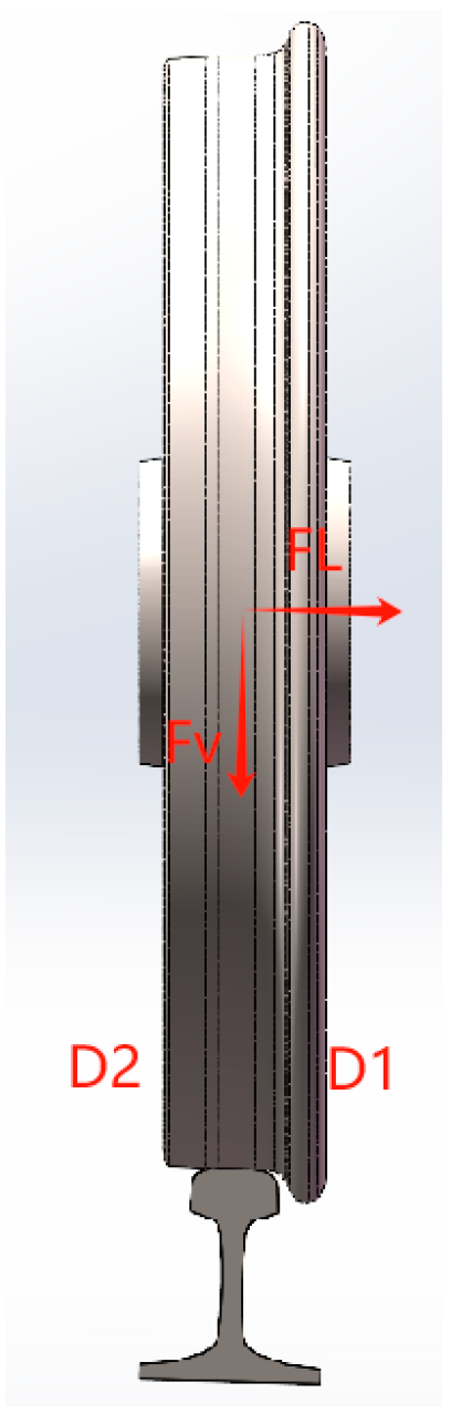
2.1. Analysis of Wheel–Rail Contact Forces

As illustrated in Figure 1, the wheel–rail contact forces include lateral forces, vertical forces, and longitudinal forces. Maintaining lateral forces within a specified range not only prevents train derailment but also ensures the train’s ability to safely negotiate curves. Longitudinal forces can provide the propulsion or braking force for the train’s advancement or deceleration. Vertical forces support the entire weight of the train. When evaluating the dynamic performance of a vehicle system, only the lateral force F_L and the vertical force F_V are considered. Under the action of the lateral force, the wheel rim is subjected to shear stress in the axial direction, resulting in substantial bending strain. Under the vertical force, the wheel rim experiences radial compressive strain along with an additional bending moment that depends on both the magnitude of the vertical force and its point of application. During normal operation on the track, the wheel is subjected to multiple forces: the lateral force, the vertical force, and an additional bending moment M. The additional moment M arises from the product of the vertical force P and the deviation x from the rolling circle. As illustrated in Figure 1, the total strain experienced by the wheel results from the linear superposition of the strains induced by the vertical force, lateral force, and additional bending moment.

Under the combined effects of lateral force F_L, vertical force F_V, and bending moment M, the strain on the surface of the wheel is a linear superposition of these three forces [16]:

$$\begin{array}{l}{X}_{\mathrm{D}1}=X_{\mathrm{V}1}+X_{\mathrm{L}1}+X_{\mathrm{M}1}\\ X_{\mathrm{D}2}=X_{\mathrm{V}2}+X_{\mathrm{L}2}+X_{\mathrm{M}2}\end{array}$$

(1)

In the above formula, $X$_D1 and $X$_D2 represent the total strain on the inner and outer surfaces of the wheel; $X$_V1 and $X$_V2 represent the strain on the inner and outer surfaces of the wheel caused by the vertical force; $X$_L1 and $X$_L2 represent the strain on the inner and outer surfaces of the wheel caused by the lateral force; and $X$_M1 and $X$_M2 represent the strain on the inner and outer surfaces of the wheel caused by the bending moment.

2.2. Decoupling Identification of Wheel–Rail Contact Loads

Due to the inability to directly measure the contact forces between the wheelset and the rail, indirect force measurement methods are often employed to determine the wheel–rail contact loads. Strain measurements on the wheel spokes are used indirectly to solve for the wheel–rail contact loads. As indicated by Equation (1), the strain at each position is influenced by the coupling effects of vertical and lateral forces. Therefore, it is necessary to decouple the vertical and lateral loads and establish a mapping relationship between the strain and these forces. Ultimately, this allows for the estimation of lateral and vertical forces from the measured strains.

To decouple and identify the lateral force while compensating for its influence, the inner and outer strains of the wheel can be solved to eliminate the effect of the vertical force. The specific expression for this process is as follows:

$$X_{\mathrm{V}}=X_{\mathrm{V}1}=X_{\mathrm{V}2}={\displaystyle \frac{1}{2}}(X_{\mathrm{D}1}+X_{\mathrm{D}2})$$

(2)

In the above formula, F_V represents the vertical load; X_V denotes the average strain on the inner and outer surfaces of the wheel due to the vertical load.

To decouple and identify the lateral force while compensating for the influence of the vertical force, the difference in the inner and outer strains of the wheel can be utilized. The strain induced in the wheel due to the lateral force is given by

$$X_{\mathrm{L}}=X_{\mathrm{L}1}=-X_{\mathrm{L}2}={\displaystyle \frac{1}{2}}(X_{\mathrm{D}1}-X_{\mathrm{D}2})-X_{\mathrm{M}1}$$

(3)

Although the above equation eliminates the influence of vertical loads, it does not account for the effects of the offset moment X_M1. The magnitude of the offset moment is determined by the vertical load on the wheel and the extent of offset at the wheel–rail contact point. However, given that the offset moment is considerably smaller compared to the bending moment generated by the lateral force, its impact can be disregarded [16]. Consequently, Equation (3) can be simplified as follows:

$$X_{\mathrm{L}}={\displaystyle \frac{1}{2}}(X_{\mathrm{D}1}-X_{\mathrm{D}2})$$

(4)

Through the aforementioned analysis, it is evident that the vertical load is related only to the sum of the inner and outer strains, while the lateral load is associated solely with the difference between the inner and outer strains.

Therefore, we have successfully implemented the decoupled identification of vertical and lateral forces. The traditional method for decoupling wheel–rail loads relies on deterministic assumptions. However, real-world engineering problems involve uncertainties. Hence, it is essential to analyze the decoupled identification of wheel–rail loads in the presence of such uncertainties.

3. Interval Uncertainty Analysis of Wheel–Rail Loads

For wheel–rail contact load analysis with uncertainties, a novel method named IFOPCE is proposed to propagate the uncertainty in wheel–rail contact systems. In IFOPCE, the PCE is first utilized to approximate the relationship between strain responses, wheel–rail loads, and uncertain variables. The expansion coefficients are calculated using LHS. To efficiently decouple the wheel–rail loads, the relationship between load and strain is established based on the first-order PCE.

3.1. Interval Model

For parameters such as the material properties and strain of the wheel, there is often insufficient sample data to determine their precise probability density functions; only upper and lower bounds can be obtained. Interval models treat uncertain parameters as unknown but bounded interval numbers, requiring only the range of parameter distribution for calculations. Therefore, an interval model is adopted to describe the uncertainties in the material properties and strain of the wheel.

In the interval model, uncertain parameters are represented as interval variables with known ranges. Let x be an interval variable with a range of $\left[\underset{¯}{x},\overline{x}\right]$, where $\underset{¯}{x}$ and $\overline{x}$ denote the lower and upper bounds of the interval, respectively. The mean value x^c and the radius $\Delta x$ of the interval variable b can be expressed as

$${\mathrm{x}}^c={\displaystyle \frac{\underset{¯}{x}+\overline{x}}{2}},\Delta x={\displaystyle \frac{-\underset{¯}{x}+\overline{x}}{2}},\Delta x^I\in \left[-\Delta x,\Delta x\right]$$

(5)

3.2. Polynomial Chaos Expansion-Based Interval Uncertainty Analysis Method

Due to the complexity of the wheel–rail model, it is essential to quantify and analyze the uncertainties that directly affect the output. The PCE method demonstrates significant potential for such analysis. The PCE method is particularly suitable for simulation experiments where the stochastic output response can be accurately approximated with a small number of polynomial expansion terms, especially when only a few random input variables are involved. This study applies the PCE method to the interval uncertainty analysis of wheel–rail load identification [17]:

$$y=F(x)={\displaystyle \sum _{\alpha \in {{\rm N}}^n}{\beta }_{\alpha }}{\psi }_{\alpha }(x)$$

(6)

In the above equation, $\alpha =({\alpha }_1,\dots ,{\alpha }_n),({\alpha }_i\ge 0)$ indicates the multi-index composed of the polynomial orders corresponding to each random variable; ${\beta }_{\alpha }$ is the expansion coefficient of the multivariate orthogonal polynomial basis; and ${\psi }_{\alpha }$ represents the tensor product of univariate orthogonal polynomials.

The probability distribution of the random variables in Equation (6) can be arbitrary. Based on this, a general orthogonal polynomial chaos expansion was later developed, with the orthogonal polynomial basis constructed using the following three-term recurrence formula:

$${\psi }_{-1}(x)=0$$

(7)

$${\psi }_0(x)=1$$

(8)

$${\psi }_{k+1}(x)=(x-a_k){\psi }_k(x)-b_k{\psi }_{k-1}(x),k=0,1,2,\dots$$

(9)

In the above equations, $a_k$ and $b_k$ represent the recurrence coefficients, which can be calculated using the following formula:

$$a_k={\displaystyle \frac{〈x{\psi }_k(x),{\psi }_k(x)〉}{〈{\psi }_k(x),{\psi }_k(x)〉}},b_k={\displaystyle \frac{〈{\psi }_k(x),{\psi }_k(x)〉}{〈{\psi }_{k-1}(x),{\psi }_{k-1}(x)〉}}$$

(10)

In practical applications, to conserve computational resources, Equation (6) is typically truncated, retaining only the total order not exceeding a given p-th-order polynomial, i.e.,

$$y\approx F_p(x)={\displaystyle \sum _{\alpha \in {\lambda }_{n,p}}{\beta }_{\alpha }}{\psi }_{\alpha }(x),{\lambda }_{n,p}=\left\{\alpha \in N^n:\left|\alpha \right|\le p\right\}$$

(11)

Equation (11) is referred to as the p-th-order full polynomial chaos expansion of the model response y. The relationship between the total number of unknown coefficients after truncation, the maximum order p, and the maximum dimension n of the input variables is

$$\mathrm{card}({\lambda }_{n,p})={\displaystyle \frac{(n+p)!}{n!p!}}$$

(12)

The complex computational process and significant computational cost associated with high-order polynomial chaos expansion are unmanageable. Therefore, a first-order polynomial chaos expansion is adopted in this study, and Equation (6) is transformed as follows:

$$y\approx F_1(x)={\beta }_0+{\displaystyle \sum _{\mathrm{i}=1}^n{\beta }_i{\psi }_i(x)}$$

(13)

Equation (13) is then converted into the relationship between strain, load, and other interval vectors:

$$\mathrm{X}={\beta }_0+{\displaystyle \sum _{\mathrm{k}=1}^m{\beta }_k{\psi }_1(x)}+{\displaystyle \sum _{j=1}^l{\alpha }_j}{\psi }_1(F_j)$$

(14)

In the above equation, X represents strain, and β₀, β_k (k = 1, 2, …, m), and α_j (j = 1, 2, …, m) are the expansion coefficients of the multivariate orthogonal polynomial basis.

When only vertical or lateral load is applied separately, the above equation becomes

$${\mathrm{X}}_{\mathrm{L}}={\beta }_0+{\displaystyle \sum _{\mathrm{k}=1}^m{\beta }_k{\psi }_1(x)}+{\alpha }_1{\psi }_1(F_1)$$

(15)

$${\mathrm{X}}_{\mathrm{v}}={\beta }_0+{\displaystyle \sum _{\mathrm{k}=1}^m{\beta }_k{\psi }_1(x)}+{\alpha }_2{\psi }_1(F_2)$$

(16)

In the above equations, F₁ represents lateral load, and F₂ represents vertical load.

When it is necessary to solve for the separately applied loads based on strain and other interval vectors, the equation is transformed into a formula involving interval vectors, strain, and load:

$$F_1={\displaystyle \frac{X_L-{\beta }_0-{\displaystyle \sum _{k=1}^m{\beta }_k{\psi }_1(x)}}{{\alpha }_1}}+a_0+b_0$$

(17)

$$F_2={\displaystyle \frac{{\mathrm{X}}_{\mathrm{v}}-{\beta }_0-{\displaystyle \sum _{k=1}^m{\beta }_k{\psi }_1(x)}}{{\alpha }_2}}+a_0+b_0$$

(18)

To improve estimation accuracy and computational efficiency, this paper employs LHS to generate samples, ensuring the results of the analysis are both accurate and reliable. Let ${\Re }_1=\{{\xi }_1^{(1)}\},{\xi }_1^{(2)},\dots \left.\right\}$ and ${\Re }_0=\{{\xi }_0^{(1)}\},{\xi }_0^{(2)},\dots \left.\right\}$ be defined as the sample pools composed of selected and unselected samples, respectively. The initial samples are generated using LHS. The distance metric is expressed as

$${\varsigma }^n={\displaystyle \sum _{i=1}^{N_{{\Re }_1}}{\displaystyle \sum _{j=i+1}^{N_{{\Re }_1}}D({\xi }_1^{(i)}}},{\xi }_1^{(j)}{)}^{-n}$$

(19)

where $N_{{\Re }_1}$ represents the number of samples, and n is a large positive number, with n = 50 used in this study; $D({\xi }_1^{(i)},{\xi }_1^{(j)})$ denotes the Minkowski distance.

The sample selection formula is given by

$$\begin{array}{rr}& {\widehat{\xi }}_0^{k+1}=\underset{{\xi }_0^{k=1}\in {\mathfrak{R}}_0^{\left(k\right)}}{\mathrm{m}\mathrm{i}\mathrm{n}} {\left({\tilde{D}}_{k+1}\right)}^{1/n}\\ & {\tilde{D}}_{k+1}={\displaystyle \sum _{i=1}^{N_{{\mathfrak{R}}_1}^{\left(k\right)}}} D{\left({\xi }_1^{\left(i\right)},{\xi }_1^{k+1}\right)}^{-n}\end{array}$$

(20)

and the values for the Minkowski distance, distance metric, etc., can be found in the paper by STEIN M [18].

3.3. Interval Response Analysis

Based on the IFOPCE method established in Section 3.2, we can quickly calculate the maximum and minimum values of the loads, as follows:

$${\mathrm{F}}_{\mathrm{Lmax}}=\underset{x\in x^I}{\max }\left\{{\displaystyle \frac{X_L-{\beta }_0-{\displaystyle \sum _{k=1}^m{\beta }_k{\psi }_1(x)}}{{\alpha }_1}}+a_0+b_0\right\}$$

(21)

$${\mathrm{F}}_{\mathrm{Lmin}}=\underset{x\in x^I}{\min }\left\{{\displaystyle \frac{X_L-{\beta }_0-{\displaystyle \sum _{k=1}^m{\beta }_k{\psi }_1(x)}}{{\alpha }_1}}+a_0+b_0\right\}$$

(22)

$${\mathrm{F}}_{\mathrm{Vmax}}=\underset{x\in x^I}{\max }\left\{{\displaystyle \frac{X_{\mathrm{V}}-{\beta }_0-{\displaystyle \sum _{k=1}^m{\beta }_k{\psi }_1(x)}}{{\alpha }_1}}+a_0+b_0\right\}$$

(23)

$${\mathrm{F}}_{\mathrm{Vmin}}=\underset{x\in x^I}{\min }\left\{{\displaystyle \frac{X_{\mathrm{V}}-{\beta }_0-{\displaystyle \sum _{k=1}^m{\beta }_k{\psi }_1(x)}}{{\alpha }_1}}+a_0+b_0\right\}$$

(24)

By using Equations (15)–(24), we can obtain the maximum and minimum values of the wheel–rail loads. In summary, the computational procedure of the IFOPCE method proposed in this paper is as follows:

• Uncertain parameters were identified: There are many uncertain parameters for the decoupling identification of wheel–rail contact loads, such as Young’s modulus and strain.
• The PCE algorithm was used to perform the calculation and obtain a large number of strain samples according to Equation (20).
• The approximate function was constructed based on Equations (15) and (16) to establish the relationship between strain and load, as well as Young’s modulus.
• The strain in the simulation model was compared with that obtained from the IFOPCE in step 3 to verify the accuracy of the IFOPCE.
• Equations (17) and (18) were used to construct an approximate function that determines the relationship between load and strain, as well as Young’s modulus.
• Strain and Young’s modulus were treated as interval variables, and the load response interval was derived by substituting them into the IFOPCE in step 5 for interval accuracy analysis.
• The influence of parameter uncertainty was analyzed: The impact of parameter uncertainties on the uncertainty in load identification was analyzed through the examples.

4. Numerical Examples

The feasibility of the interval uncertainty analysis method for wheel–rail load identification, based on IFOPCE as proposed in this study, was validated through a numerical scenario. Furthermore, we analyzed how parameter uncertainties affect the uncertainty of the load.

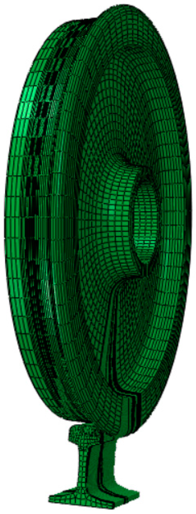
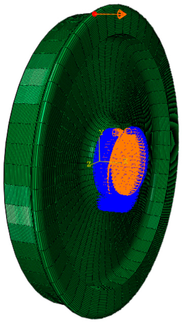
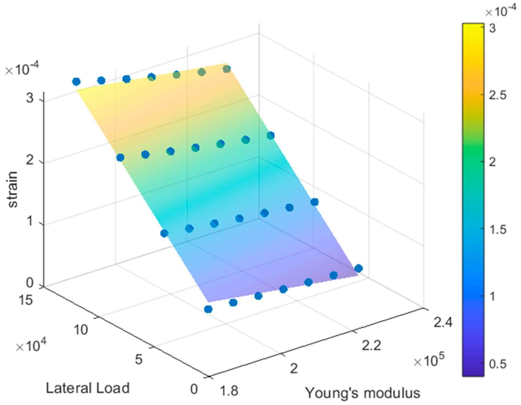
4.1. Finite Element Model

To address uncertainties related to structural defects and material variability in FEM modeling, we have reviewed advanced approaches that can improve the accuracy and reliability of our analysis. One such approach is the energy functional-based method, which provides a better characterization of internal imperfections and defects by reducing the impact of structural simplifications [19]. This method offers a robust framework for dealing with uncertainties and complex material behaviors, making it highly relevant to our study.

This study develops a computational model based on the actual three-dimensional dimensions of the wheel of a certain locomotive and a 60 kg/m rail [20]. The locomotive wheel has a diameter of 920 mm and features an LMA-type tread. Due to the complexity of direct modeling in ABAQUS, SolidWorks was used for CAD modeling. The components were first modeled in SolidWorks and then imported into Hypermesh for mesh generation. Meshing is a critical step in the preprocessing phase, as the quality of the mesh directly influences the accuracy of the computational results. In Hypermesh, the element size was set to 5, with the element density maintained at the default value of 1. Approximately 120 finite elements were generated per wheel [21]. Finally, the components were imported into ABAQUS, where material properties were assigned to the model. The wheel material was specified as steel with the following properties:

Young’s Modulus: 2.1 × 10⁵ N/m²

Poisson’s Ratio: 0.3

Material Density: 7.85 × 10³ kg/m³

The three-dimensional modeling results are shown in Figure 2.

Computer simulations were used to apply loads to the wheel, with concentrated forces representing the forces exerted by the rail on the wheel [22]. Static force calibration methods, similar to those used in laboratory tests for force-measuring wheel sets, were employed to simulate static force loading on the wheel. The loading conditions were as follows:

• Lateral load F_L = 10 kN; vertical load F_V = 0;
• Lateral load F_L = 0; vertical load F_V = 10 kN.

The two loading scenarios are shown in Figure 3 and Figure 4.

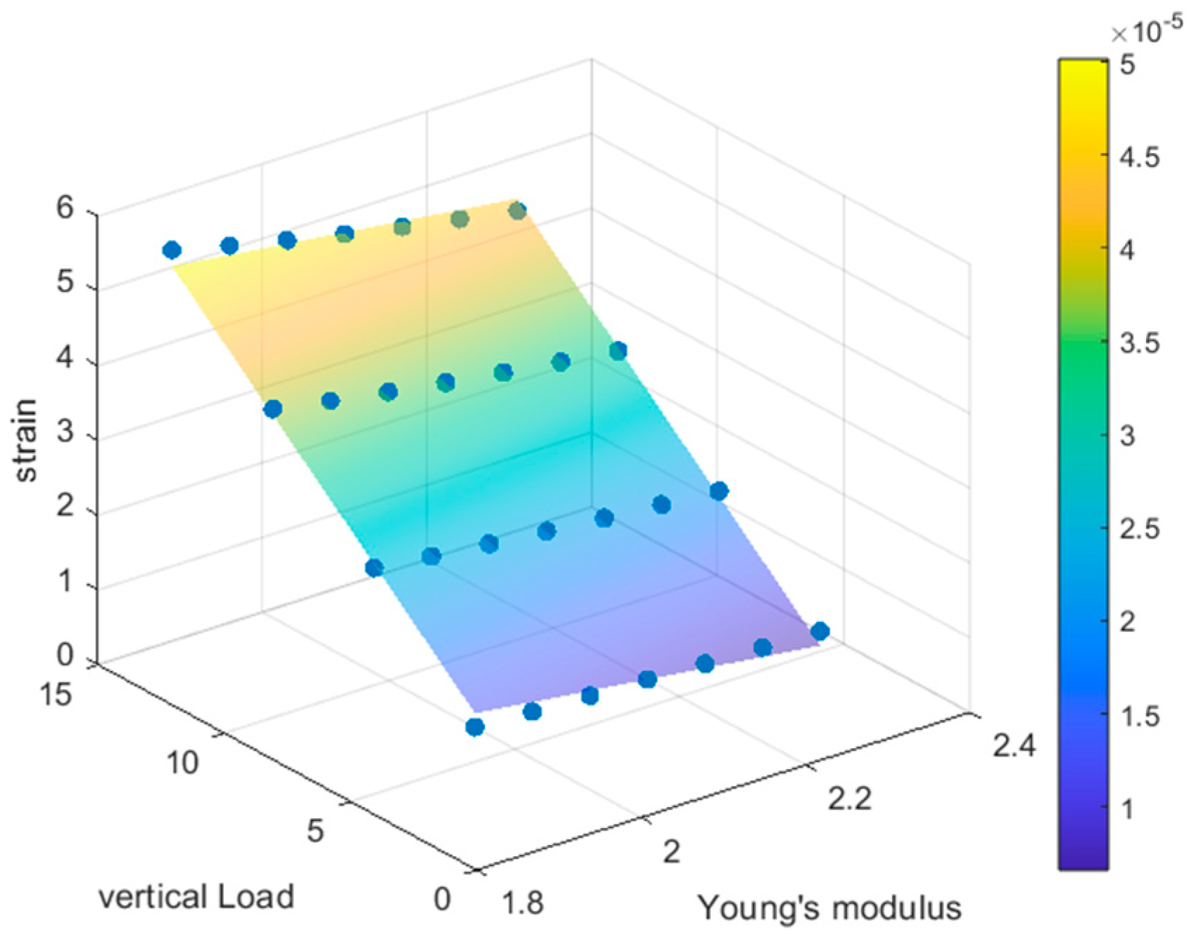
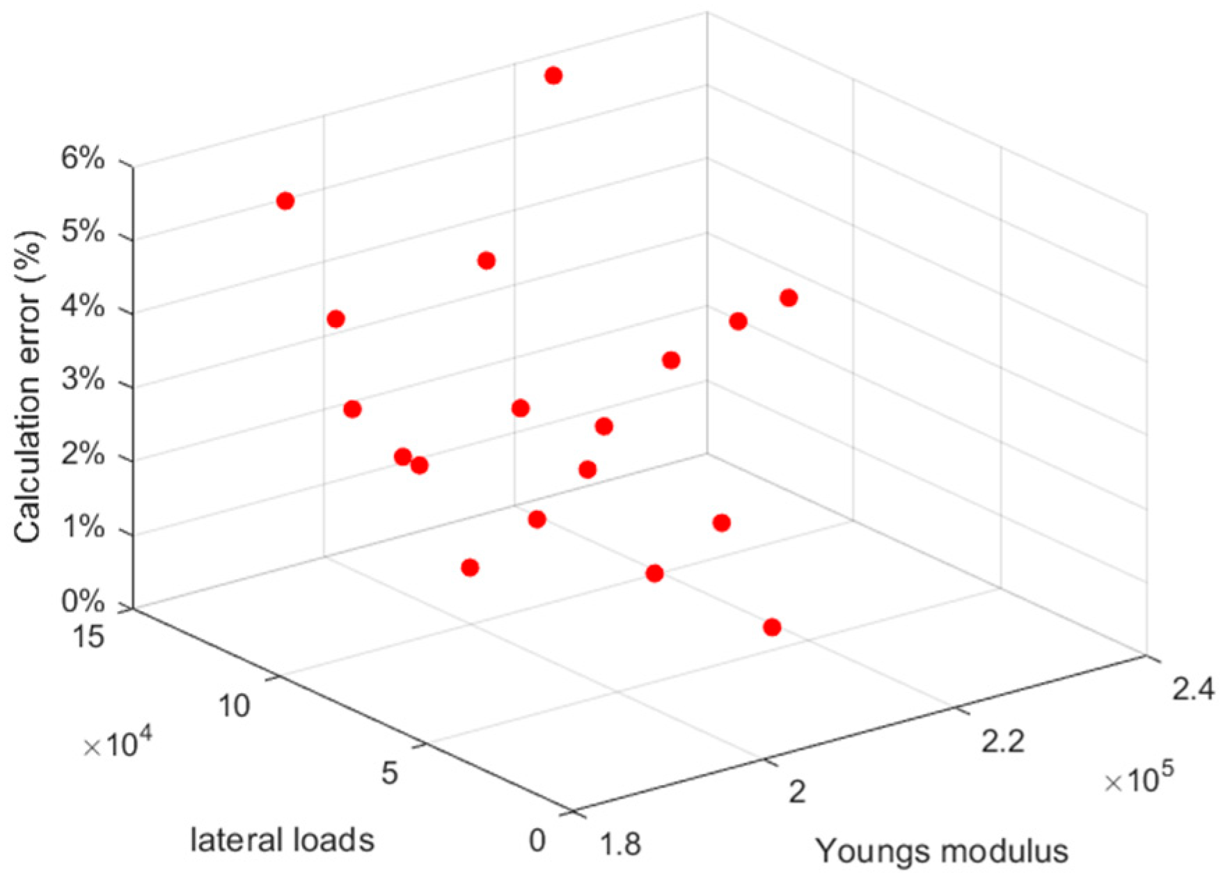
4.2. Accuracy Analysis of IFOPCE

To validate the accuracy of the IFOPCE method, we used a scanning method to verify the accuracy of the proxy model. This study calculates the vertical strain $X_{\mathrm{VSi}}$ and lateral strain $X_{\mathrm{LSi}}$ using the Finite Element Method and compares them with the vertical strain $X_{\mathrm{VI}}$ and lateral strain $X_{\mathrm{LI}}$ obtained by the IFOPCE method, as shown in Figure 5 and Figure 6.

To more clearly analyze the accuracy of IFOPCE, the computational error of the IFOPCE is defined as follows [23]:

$$\Delta X={\displaystyle \frac{X_{Su}-X_{Si}}{X_{Si}}}\times 100\%$$

(25)

In the formula, $X_{Su}$ represents the strain calculated by the IFOPCE, and $X_{Si}$ represents the strain obtained from the simulation model. The accuracy verification of the IFOPCE is illustrated in Figure 7 and Figure 8.

As shown in Figure 7 and Figure 8, the errors between the IFOPCE and the simulation model under vertical and lateral loads are approximately 5%. Therefore, the IFOPCE derived using the PCE demonstrates a high level of computational accuracy.

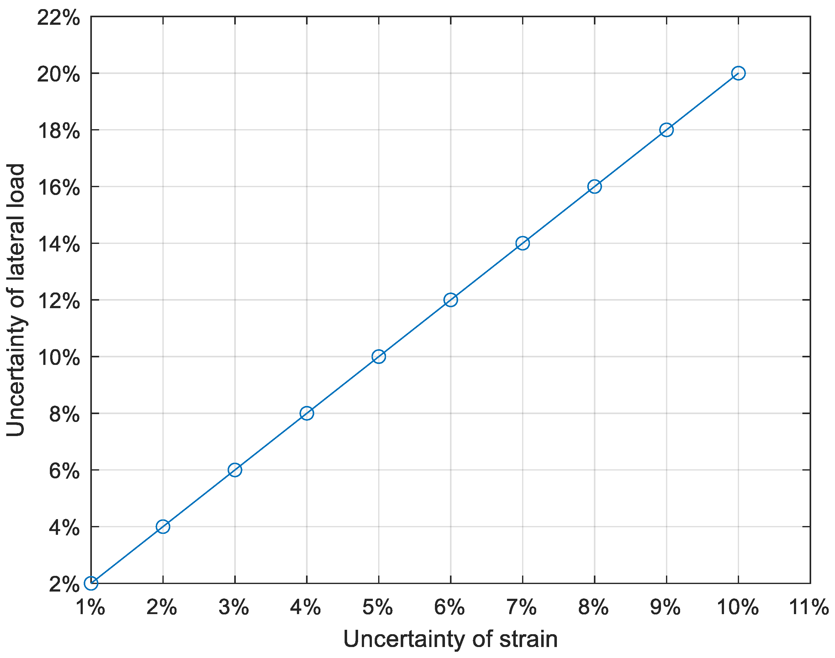
4.3. Influence of Parameter Uncertainty on Load Identification Uncertainty

Young’s modulus and strain were set as uncertain parameters, one at a time, and it was investigated how these parameter uncertainties affect the uncertainty in load identification.

To analyze the impact of input parameter uncertainties on response uncertainties, the following uncertainty calculation formulas are defined:

$$x^{\mathrm{I}}=x^m+\Delta x\times e^{\mathrm{I}}$$

(26)

In the above formula, $x^I$ represents the interval variable, $x^m$ is the midpoint of the interval, $\Delta x$ represents the uncertainty of the interval variable, and $e^I$ denotes the unit interval variable [−1, 1].

To investigate the influence of uncertainty in Young’s modulus on the identification uncertainty of vertical and lateral loads, Young’s modulus E was defined as an interval variable [24]. The uncertainty of Young’s modulus is set to range from 1% to 10% [25]. Based on this setting, the uncertainties of the vertical and lateral loads are presented in

Table 1. The influence of Young’s modulus uncertainty on vertical load uncertainty.

Uncertainty of Young’s Modulus	The Variation Range of Young’s Modulus	XV	${\mathbf{F}}_{\mathbf{V}}$	Uncertainty of Load
1%	[207,900, 212,100]	1.57 × 10−5	[48,870, 50,676.2]	3.6%
2%	[205,800, 214,200]	1.57 × 10−5	[47,966.9, 51,579.3]	7.3%
3%	[203,700, 216,300]	1.57 × 10−5	[47,063.8, 52,482.3]	10.9%
4%	[201,600, 218,400]	1.57 × 10−5	[46,160.8, 53,385.4]	14.5%
5%	[199,500, 220,500]	1.57 × 10−5	[45,257.7, 54,288.5]	18.1%
6%	[197,400, 222,600]	1.57 × 10−5	[44,354.6, 55,191.6]	21.8%
7%	[195,300, 224,700]	1.57 × 10−5	[43,451.5, 56,094.7]	25.4%
8%	[193,200, 226,800]	1.57 × 10−5	[42,548.4, 56,997.8]	29%
9%	[191,100, 228,900]	1.57 × 10−5	[41,645.3, 57,900.9]	32.7%
10%	[189,000, 231,000]	1.57 × 10−5	[40,742.3, 58,803.9]	36.3%

and

Table 2. The influence of Young’s modulus uncertainty on lateral load uncertainty.

Uncertainty of Young’s Modulus	The Variation Range of Young’s Modulus	XL	${\mathbf{F}}_{\mathbf{L}}$	Uncertainty of Load
1%	[207,900, 212,100]	1.33 × 10−4	[68,923.6, 70,729.6]	2.6%
2%	[205,800, 214,200]	1.33 × 10−4	[68,020.6, 71,632.6]	5.2%
3%	[203,700, 216,300]	1.33 × 10−4	[67,117.5, 72,535.6]	7.8%
4%	[201,600, 218,400]	1.33 × 10−4	[66,214.5, 73,438.6]	10.3%
5%	[199,500, 220,500]	1.33 × 10−4	[65,311.5, 74,341.6]	12.9%
6%	[197,400, 222,600]	1.33 × 10−4	[64,408.5, 75,244.6]	15.5%
7%	[195,300, 224,700]	1.33 × 10−4	[63,505.5, 76,147.7]	18.1%
8%	[193,200, 226,800]	1.33 × 10−4	[62,602.5, 77,050.7]	20.7%
9%	[191,100, 228,900]	1.33 × 10−4	[61,699.5, 77,953.7]	23.3%
10%	[189,000, 231,000]	1.33 × 10−4	[60,796.5, 78,856.7]	25.9%

, respectively.

To better illustrate the impact of uncertainty in Young’s modulus on the uncertainties of vertical and lateral loads, the data from Table 1 and Table 2 are graphically presented in Figure 9.

As shown in Figure 9, the uncertainty in Young’s modulus has a more significant impact on the uncertainty of the vertical load than on that of the lateral load.

To investigate the impact of strain uncertainty on the identification uncertainty of vertical and lateral loads, strain was defined as an interval variable [26]. Based on this definition, the uncertainties of vertical and lateral loads are presented in

Table 3. The influence of strain uncertainty on vertical load uncertainty.

Uncertainty of Strain	The Variation Range of Strain	E	${\mathbf{F}}_{\mathbf{V}}$	Uncertainty of Load
1%	[1.5543 × 10−5, 1.5857 × 10−5]	210,000	[49,275.3, 50,270.9]	2%
2%	[1.5386 × 10−5, 1.6014 × 10−5]	210,000	[48,777.5, 50,768.7]	4%
3%	[1.5229 × 10−5, 1.6171 × 10−5]	210,000	[48,279.6, 51,266.5]	6%
4%	[1.5072 × 10−5, 1.6328 × 10−5]	210,000	[47,781.8, 51,764.4]	8%
5%	[1.4915 × 10−5, 1.6485 × 10−5]	210,000	[47,284.0, 52,262.2]	10%
6%	[1.4758 × 10−5, 1.6642 × 10−5]	210,000	[46,786.2, 52,760.0]	12%
7%	[1.4601 × 10−5, 1.6799 × 10−5]	210,000	[46,288.4, 53,257.8]	14%
8%	[1.4444 × 10−5, 1.6956 × 10−5]	210,000	[45,790.6, 53,755.6]	16%
9%	[1.4287 × 10−5, 1.7113 × 10−5]	210,000	[45,292.8, 54,253.4]	18%
10%	[1.413 × 10−5, 1.727 × 10−5]	210,000	[44,794.9, 54,751.3]	20%

and

Table 4. The influence of strain uncertainty on lateral load uncertainty.

Uncertainty of Strain	The Variation Range of Strain	E	${\mathbf{F}}_{\mathbf{L}}$	Uncertainty of Load
1%	[1.3167 × 10−4, 1.3433 × 10−4]	210,000	[69,128.3, 70,524.8]	2%
2%	[1.3034 × 10−4, 1.3566 × 10−4]	210,000	[68,430.0, 71,223.1]	4%
3%	[1.2901 × 10−4, 1.3699 × 10−4]	210,000	[67,731.8, 71,921.4]	6%
4%	[1.2768 × 10−4, 1.3832 × 10−4]	210,000	[67,033.5, 72,619.6]	8%
5%	[1.2635 × 10−4, 1.3965 × 10−4]	210,000	[66,335.2, 73,317.9]	10%
6%	[1.2502 × 10−4, 1.4098 × 10−4]	210,000	[65,637.0, 74,016.2]	12%
7%	[1.2369 × 10−4, 1.4231 × 10−4]	210,000	[64,938.7, 74,714.4]	14%
8%	[1.2236 × 10−4, 1.4364 × 10−4]	210,000	[64,240.4, 75,412.7]	16%
9%	[1.2103 × 10−4, 1.4497 × 10−4]	210,000	[63,542.2, 76,111.0]	18%
10%	[1.197 × 10−4, 1.463 × 10−4]	210,000	[62,843.9, 74,809.2]	20%

, respectively.

Similarly, to better illustrate the effect of strain uncertainty on the uncertainties of vertical and lateral loads, the data from Table 3 and Table 4 are graphically presented in Figure 10 and Figure 11, respectively.

As illustrated in Figure 10 and Figure 11, the impact of strain uncertainty on the uncertainty of vertical load is nearly identical to its impact on the uncertainty of lateral load.

The variations in the uncertainty of vertical load and lateral load when both Young’s modulus and strain are treated as interval variables [27] are presented in

Table 5. Effects of Young’s modulus uncertainty and strain uncertainty on vertical load uncertainty.

Uncertainty of Variables	The Variation Range of Strain	The Variation Range of Young’s Modulus	${\mathbf{F}}_{\mathbf{V}}$	Uncertainty of Load
1%	[1.5543 × 10−5, 1.5857 × 10−5]	[207,900, 212,100]	[49,275.3, 50,270.9]	5.6%
2%	[1.5386 × 10−5, 1.6014 × 10−5]	[205,800, 214,200]	[48,777.5, 50,768.7]	11.3%
3%	[1.5229 × 10−5, 1.6171 × 10−5]	[203,700, 216,300]	[48,279.6, 51,266.5]	16.9%
4%	[1.5072 × 10−5, 1.6328 × 10−5]	[201,600, 218,400]	[47,781.8, 51,764.4]	22.5%
5%	[1.4915 × 10−5, 1.6485 × 10−5]	[199,500, 220,500]	[47,284.0, 52,262.2]	28.1%
6%	[1.4758 × 10−5, 1.6642 × 10−5]	[197,400, 222,600]	[46,786.2, 52,760.0]	33.8%
7%	[1.4601 × 10−5, 1.6799 × 10−5]	[195,300, 224,700]	[46,288.4, 53,257.8]	39.4%
8%	[1.4444 × 10−5, 1.6956 × 10−5]	[193,200, 226,800]	[45,790.6, 53,755.6]	45.0%
9%	[1.4287 × 10−5, 1.7113 × 10−5]	[191,100, 228,900]	[45,292.8, 54,253.4]	50.7%
10%	[1.413 × 10−5, 1.727 × 10−5]	[189,000, 231,000]	[44,794.9, 54,751.3]	56.3%

and

Table 6. Effects of Young’s modulus uncertainty and strain uncertainty on lateral load uncertainty.

Uncertainty of Variables	The Variation Range of Strain	The Variation Range of Young’s Modulus	${\mathbf{F}}_{\mathbf{L}}$	Uncertainty of Load
1%	[1.3167 × 10−4, 1.3433 × 10−4]	[207,900, 212,100]	[68,225.3, 71,427.9]	4.6%
2%	[1.3034 × 10−4, 1.3566 × 10−4]	[205,800, 214,200]	[66,624.0, 73,029.1]	9.2%
3%	[1.2901 × 10−4, 1.3699 × 10−4]	[203,700, 216,300]	[65,022.7, 74,630.4]	13.8%
4%	[1.2768 × 10−4, 1.3832 × 10−4]	[201,600, 218,400]	[63,421.5, 76,231.7]	18.3%
5%	[1.2635 × 10−4, 1.3965 × 10−4]	[199,500, 220,500]	[61,820.2, 77,833.0]	22.9%
6%	[1.2502 × 10−4, 1.4098 × 10−4]	[197,400, 222,600]	[60,218.9, 79,434.2]	27.5%
7%	[1.2369 × 10−4, 1.4231 × 10−4]	[195,300, 224,700]	[58,617.6, 81,035.5]	32.1%
8%	[1.2236 × 10−4, 1.4364 × 10−4]	[193,200, 226,800]	[57,016.4, 82,636.8]	36.7%
9%	[1.2103 × 10−4, 1.4497 × 10−4]	[191,100, 228,900]	[55,415.1, 84,238.1]	41.3%
10%	[1.197 × 10−4, 1.463 × 10−4]	[189,000, 231,000]	[53,813.8, 85,839.3]	45.9%

, respectively.

To better illustrate the effect of uncertainties in Young’s modulus and strain on the uncertainties of vertical and lateral loads, the data from Table 5 and Table 6 are presented graphically in Figure 12.

As shown in Figure 12, uncertainties in Young’s modulus and strain have a more significant effect on the uncertainty of vertical load than on that of lateral load.

The results of the three case studies clearly demonstrate that uncertainties in Young’s modulus and strain notably affect wheel–rail loads. Furthermore, in our study, we have addressed the combined effect of strain uncertainty and Young’s modulus uncertainty on load uncertainty, as shown in Figure 12. The figure illustrates that the combined effect of these uncertainties on the load uncertainty is the product of their individual effects. This approach provides a clear understanding of how the uncertainties interact and influence the overall load uncertainty. Therefore, it is essential to account for parameter uncertainties when identifying wheel–rail loads.

While our method offers valuable insights into the uncertainty analysis of wheel–rail contact loads, it has limitations. First-order polynomial expansion, though computationally efficient, may not handle highly non-linear uncertainties, restricting its application to problems with high non-linearity. Additionally, the method is designed for static or quasi-static scenarios and cannot be directly extended to dynamic loads or time-varying conditions without significant modifications.

Our study highlights the importance of addressing uncertainties and complex conditions in wheel–rail load analysis. Current methods often face limitations in handling parameter sensitivity and validation. Future research could benefit from exploring advanced uncertainty handling methods, such as the dynamic model proposed by Angiulli et al. [28], which demonstrates the potential for more accurate stress distribution and dynamic response modeling under complex conditions. Such advancements could significantly improve the reliability and accuracy of wheel–rail load analysis.

5. Conclusions

This paper proposed a method named IFOPCE for the uncertainty analysis of wheel–rail contact loads, which can decouple the variational range of wheel–rail contact loads. In IFOPCE, the uncertainties are dealt with interval model. The wheel–rail contact load decoupled model is derived based on IFOPCE. The proposed method is used to analyze the uncertainties in a wheel–rail contact system. The main conclusions are as follows:

• The proposed IFOPCE method can effectively obtain the variational range of the vertical and lateral forces of wheel–rail contact, which means the first-order polynomial expansion is suitable for interval uncertainty analysis of wheel–rail contact systems.
• The uncertainty of parameters such as Young’s modulus and strain has a significant effect on the uncertainty of wheel–rail load identification. Therefore, it is necessary to consider parameter uncertainties for identifying wheel–rail contact loads.

References

1. Smith, J.; Doe, A. Ground-based measurement techniques for rail vehicle load identification. J. Rail Transp. Eng. 2022, 15, 234–250. [Google Scholar]
2. Brown, L.; Green, M. On-board monitoring systems for dynamic load assessment in rail vehicles. Veh. Syst. Dyn. 2023, 61, 567–585. [Google Scholar]
3. Jónsson, J.G.; Svensson, E.; Christensen, J.T. Validation of strain gauges for rail stress measurement. IEEE/ASME Trans. Mechatron. 1997, 2, 180–187. [Google Scholar]
4. Zhao, G.; Tian, Y.; Liu, T.; Zhao, G. Development of a continuous monitoring system for vertical forces on railway tracks. J. Sound Vib. 2000, 234, 819–836. [Google Scholar]
5. Huang, H. Enhanced understanding of vertical force testing and development of a new detection system. J. Transp. Eng. 2005, 131, 411–420. [Google Scholar]
6. Zhou, W.; Fang, C.; Han, T.; Li, G. A new track-side measurement method for high-precision positioning in railway track monitoring. J. Mod. Transp. 2010, 18, 177–183. [Google Scholar]
7. Zhang, Y. Introduction of fiber Bragg grating sensing technology to improve the stability and reliability of measurement systems. Sens. Actuators A Phys. 2015, 227, 108–115. [Google Scholar]
8. Matsumoto, A. Use of non-contact gap sensors to measure lateral forces, simplifying system installation and maintenance. JSME Int. J. Ser. C Mech. Syst. Mach. Elem. Manuf. 2008, 51, 747–753. [Google Scholar]
9. Pedro, U.; Escalona, J. Comparative study of different measurement methods and exploration of laser as an alternative. Meas. Sci. Technol. 2014, 25, 125202. [Google Scholar]
10. Ren, Y. Application of state space theory to make wheel-rail force calculation more efficient. Mech. Syst. Signal Process. 2017, 94, 256–270. [Google Scholar]
11. Le Maître, O.P.; Knio, O.M. Spectral Methods for Uncertainty Quantification: With Applications to Computational Fluid Dynamics; Springer: Berlin/Heidelberg, Germany, 2019. [Google Scholar]
12. Ghanem, R.G.; Spanos, P.D. Stochastic Finite Elements: A Spectral Approach. J. Eng. Mech. 2021, 147, 04021001. [Google Scholar]
13. Jakeman, J.D.; Eldred, M.S.; Sargsyan, K. Enhancing polynomial chaos expansions with adaptive sparse grids. SIAM J. Sci. Comput. 2020, 42, A1667–A1690. [Google Scholar]
14. Liu, Y.; Ghanem, R.G. Data-driven polynomial chaos expansion for machine learning regression. J. Comput. Phys. 2020, 410, 109387. [Google Scholar]
15. Chen, S.; Lian, H.; Yang, X. Interval static displacement analysis for structures with interval parameters. Int. J. Numer. Methods Eng. 2002, 53, 393–407. [Google Scholar] [CrossRef]
16. Zhu, T.; Wang, X.; Wu, J.; Zhang, J.; Xiao, S.; Lu, L.; Yang, B.; Yang, G. Comprehensive identification of wheel-rail forces in railway vehicles based on time-domain and machine learning methods. Mech. Syst. Signal Process. 2024, 222, 111635. [Google Scholar] [CrossRef]
17. Wiener, N. The homogeneous chaos. Am. J. Math. 1938, 60, 897–936. [Google Scholar] [CrossRef]
18. Stein, M. Large sample properties of simulations using Latin hypercube sampling. Technometrics 1987, 29, 143–151. [Google Scholar] [CrossRef]
19. Versaci, M.; Laganà, F.; Morabito, F.C.; Palumbo, A.; Angiulli, G. Adaptation of an Eddy Current Model for Characterizing Subsurface Defects in CFRP Plates Using FEM Analysis Based on Energy Functional. Mathematics 2024, 12, 2854. [Google Scholar] [CrossRef]
20. Wen, T.; He, J.; Zhang, C.; He, J. wheel–rail contact force for a heavy-load train can be measured using a collaborative calibration algorithm. Information 2024, 15, 535. [Google Scholar] [CrossRef]
21. Zhang, P.; Moraal, J.; Li, Z. Design, calibration and validation of a wheel-rail contact force measurement system in V-Track. Measurement 2021, 175, 109105. [Google Scholar] [CrossRef]
22. Yang, C.; Tian, G.; Robinson, M.; Ibrahim, E.T. Wheel-rail force measurement based on wireless LC resonance sensing. IEEE Sens. J. 2023, 23, 17470–17479. [Google Scholar] [CrossRef]
23. Bruni, S.; Meijaard, J.P.; Rill, G.; Schwab, A.L. State-of-the-art and challenges of railway and road vehicle dynamics with multibody dynamics approaches. Multibody Syst. Dyn. 2020, 49, 1–32. [Google Scholar] [CrossRef]
24. Liu, Q.; Lei, X.; Rose, J.G.; Chen, H.-P.; Feng, Q.; Luo, X. Vertical wheel-rail force waveform identification using wavenumber domain method. Mech. Syst. Signal Process. 2021, 159, 107784. [Google Scholar] [CrossRef]
25. Jiang, C.; Wang, S.; Wang, B.Q.; Zhang, J.H.; Zhao, T.Y. Probabilistic reliability assessment of power systems with wind power based on Latin Hypercube Sampling. Trans. China Electrotech. Soc. 2016, 31, 193–206. [Google Scholar]
26. Kettler, M.; Zauchner, P.; Unterweger, H. Determination of wheel loads from runway cranes based on rail strain measurement. Eng. Struct. 2020, 213, 110546. [Google Scholar] [CrossRef]
27. Sarikavak, Y.; Goda, K. Dynamic wheel/rail interactions for high-speed trains on a ballasted track. J. Mech. Sci. Technol. 2022, 36, 689–698. [Google Scholar] [CrossRef]
28. Angiulli, G.; Calcagno, S.; De Carlo, D.; Laganá, F.; Versaci, M. Second-Order Parabolic Equation to Model, Analyze, and Forecast Thermal-Stress Distribution in Aircraft Plate Attack Wing–Fuselage. Mathematics 2020, 8, 6. [Google Scholar] [CrossRef]
Figure 1. Wheel–rail contact load.
Mathematics 13 00656 g001
Figure 2. Three-dimensional model of wheel–rail contact.
Mathematics 13 00656 g002
Figure 3. Schematic diagram of 10 kN lateral load.
Mathematics 13 00656 g003
Figure 4. Schematic diagram of 10 kN vertical load.
Mathematics 13 00656 g004
Figure 5. Strain response range under vertical force.
Mathematics 13 00656 g005
Figure 6. Strain response range under lateral force.
Mathematics 13 00656 g006
Figure 7. Error plot of IFOPCE under vertical load.
Mathematics 13 00656 g007
Figure 8. Error plot of IFOPCE under lateral load.
Mathematics 13 00656 g008
Figure 9. The influence of uncertainty in Young’s modulus on uncertainty under different loads.
Mathematics 13 00656 g009
Figure 10. The influence of strain uncertainty on vertical load uncertainty.
Mathematics 13 00656 g010
Figure 11. The influence of strain uncertainty on lateral load uncertainty.
Mathematics 13 00656 g011
Figure 12. The influence of uncertainty in variables on uncertainty under different loads.
Mathematics 13 00656 g012