Output Feedback Optimal Control for Discrete-Time Singular Systems Driven by Stochastic Disturbances and Markov Chains

Abstract

This paper delves into the exploration of the indefinite linear quadratic optimal control (LQOC) problem for discrete-time stochastic singular systems driven by discrete-time Markov chains. Initially, the conversion of the indefinite LQOC problem mentioned above for stochastic singular systems into an equivalent problem of normal stochastic systems is executed through a sequence of transformations. Following this, the paper furnishes sufficient and necessary conditions for resolving the transformed LQOC problem with indefinite matrix parameters, alongside optimal control strategies ensuring system regularity and causality, thereby establishing the solvability of the optimal controller. Additionally, conditions are derived to verify the definiteness of the transformed LQOC problem and the uniqueness of solutions for the generalized Markov jumping algebraic Riccati equation (GMJARE). The study attains optimal controls and nonnegative cost values, guaranteeing system admissibility. The results of the finite horizon are extended to the infinite horizon. Furthermore, it introduces the design of an output feedback controller using the LMI method. Finally, a demonstrative example demonstrates the validity of the main findings.

1. Introduction

Singular systems (also referred to as implicit or descriptor or combined differential and algebraic systems) are often more appropriate for modeling real-world systems such as those found in mechanics, biology, economics, and chemistry, etc. [1,2,3,4]. Recent academic studies on singular systems have prominently emphasized investigations into stability analysis, fuzzy control methodologies, quantized regulation techniques, adaptive control strategies, and related domains [5,6,7]. Stochastic singular systems are widely used in power systems, financial markets, biomedicine, and robot control, etc. For example, in power systems, the system can be used to model the dynamic behavior of the grid, taking into account the effects of random fluctuations such as load variations and renewable energy intermittency, and thus improve the stability and reliability of the grid. In financial markets, stochastic singular systems can be used to model asset price fluctuations and help in risk management. In the field of biomedicine, it can be used to model the dynamic behavior of biological systems and assist in disease diagnosis and treatment. In robot control, it can be used to model the dynamic behavior of a robot and improve its adaptability in a complex environment. These applications show the reliability and importance of stochastic singular systems and provide a broad prospect for subsequent research. Furthermore, researchers have integrated Markov chains into the discrete-time singular systems, adding complexity to the systems while yielding significant findings [8,9,10]. With further research, the stochastic theory has made considerable advancements in the modeling of mechanical engineering, circuit dynamics, and economic systems and has been extended to singular systems. Notably, stochastic singular systems offer superior expressiveness concerning the structural features inherent in dynamic systems when compared to conventional singular systems [11,12,13]. Incorporating stochastic disturbances within a system provides a means to emulate the uncertainties and fluctuations characteristic of real-world contexts. These uncertainties may emanate from a myriad of factors, including environmental volatility, external interferences, or inherent stochasticity within the system dynamics. By integrating stochastic disturbances, a more accurate evaluation of the system’s resilience, equilibrium, and capacity to accommodate diverse environmental stimuli can be achieved. Hence, the examination of stochastic singular systems driven by discrete-time Markov chains bears substantial pragmatic implications.

Reference [14] pioneered the LQOC problem, significantly influencing modern control theory. On the one hand, the LQOC problem provides a framework for optimizing controller design by minimizing a quadratic cost function, thereby achieving a balance between system stability, performance, and robustness. On the other hand, the LQOC problem studied in this paper is to adjust the weights of system states and inputs in the cost function according to practical needs, allowing for flexible optimization of system performance metrics such as response speed, stability, and energy consumption. Hence, the LQOC problem is currently being applied in various dynamic systems, including mechanical, electrical, and control systems, with notable applications in engineering, robotics, aerospace, and other fields [15,16]. Simultaneously, the Riccati equation stands as a pivotal tool in addressing the LQOC problem in the discrete-time case. By solving the Riccati equation, the linear feedback optimal controller in the discrete time case was obtained, and the optimal control of the studied system was finally realized [17,18]. Recently, the study of the LQOC problem has attracted the attention of many scholars. Reference [19] centered on the LQOC problem applied to discrete-time Markovian jumping systems (DTMJSs), with a particular emphasis on constraining control actions within a suitable subspace. Reference [20] concerned singular DTMJSs in infinite and finite horizons to address the LQOC problem with indefinite parameters. References [21,22] analyzed the LQOC problem in fractional-order discrete systems. Recent works in this area have shown that despite weight matrices Q and R having certain uncertainties in the stochastic system, the associated stochastic LQOC problem possibly still be well-posed. In discrete-time LQOC problems, positive definiteness, which was necessary for the control weighting matrix, will not be a mandatory condition, and it may even be negative in the presence of uncertainty factors within the system [23,24]. The above article fails to take into account the influence of stochastic disturbances on the system in practical applications. Thus, this paper investigated the subject where the LQOC problem of the discrete-time stochastic singular systems was affected by stochastic disturbances and discrete-time Markov chains.

Based on the above discussion, we investigated discrete-time stochastic singular systems with stochastic disturbances and discrete-time Markov chains. Compared with existing studies in this field, our findings highlight the following motivations and advantages.

•

In this paper, both the state and control weighting matrices could be introduced by indefinite ones in the quadratic cost function; that is, it allows negative eigenvalues for the weighting matrix. Secondly, an equivalent transformation from the indefinite LQOC problem of stochastic singular systems to normal stochastic systems is obtained in this paper, with the condition for equivalent transformation expressed in terms of the initial coefficient matrix of singular stochastic systems, which is straightforward to verify and imposes relatively few constraints.

•

This paper introduces stochastic disturbances to simulate the actual impact of a stochastic environment on the operation of real systems while also considering the output feedback control to enhance the robustness of the closed-loop system. Additionally, for the purpose of ensuring the stochastic admissibility of the singular stochastic systems of the system under study, this paper constructs a Lyapunov function with relatively low conservatism and utilizes MATLAB’s LMI toolbox to design the controller gains.

The structure of the paper is outlined as follows. In Section 2, the transformation equivalently converts the indefinite LQOC problem of stochastic singular systems driven by discrete-time Markov chains into an indefinite LQOC problem for regular systems through a sequence of equivalent transformations. Section 3 establishes necessary and sufficient conditions for the solvability of the indefinite LQOC problem. Specifically, it proves that the corresponding optimal control strategy and optimal cost can be obtained, ensuring the regularity and causality of the resulting closed-loop system. Additionally, criteria are provided to guarantee the definiteness of the transformed LQOC problem for stochastic singular systems, and it is shown that the semi-positive definite solution to the GMJARE is unique. Furthermore, the acquisition of the optimal control gain matrix and optimal cost values is detailed, demonstrating that the resulting closed-loop system is stochastically admissible with the output feedback control. At the end of Section 3, the specific form of the optimal control gain matrix is derived using the rigorous LMI method. Finally, in Section 4, a numerical example with four Markovian switching modes is presented to validate the main results.

2. Foundation and Problem Formulation

Consider a class of discrete-time singular systems subjected to stochastic disturbances and driven by discrete-time Markov chains:

$$\left\{\begin{array}{cc}E{x}_{k+1}=A_{\theta \left(k\right)}{x}_k+B_{\theta \left(k\right)}{u}_k+(C_{\theta \left(k\right)}{x}_k+D_{\theta \left(k\right)}{u}_k){\omega }_k,\hfill & \\ y_k=G_{\theta \left(k\right)}{x}_k+H_{\theta \left(k\right)}{\omega }_k,\hfill \end{array}\right.$$

(1)

where $x_k\in {\mathbb{R}}^n$, $u_k\in {\mathbb{R}}^m$ and $y_k\in {\mathbb{R}}^{\tilde{n}}$. The matrix $E\in {\mathbb{R}}^{n\times n}$ is singular and $\mathrm{rank}\left(E\right)=r<n$. $\theta \left(k\right)$ represents a Markov chain in discrete-time case to take values in the positive-integer set $\mathbb{L}=\{1,\cdots ,l\}$ and its transition probabilities are $p_{ij}$, which means the probability of $\theta (k+1)$ being j under $\theta \left(k\right)=i$, with $0\le p_{ij}\le 1$ and ${\sum }_{i=1}^l{p}_{ij}=1$ ($i,j\in \mathbb{L}$). All the system parameter matrices can be abbreviated as $A_i\in {\mathbb{R}}^{n\times n}$, $B_i\in {\mathbb{R}}^{n\times m}$, $C_i\in {\mathbb{R}}^{n\times n}$, $D_i\in {\mathbb{R}}^{n\times m}$, $G_i\in {\mathbb{R}}^{\tilde{n}\times n}$, $H_i\in {\mathbb{R}}^{\tilde{n}}$ for $\theta \left(k\right)=i$. Assume that $\theta \left(k\right)$ is unrelated to the initial state $x_0$. $\{{\omega }_k:k=1,2,\cdots \}$ is a one-dimensional white noise in a given complete probability space $(\Omega ,\mathcal{F},\mathbb{P})$, where ${\omega }_k$ and $\theta \left(k\right)$ are independent with each other.

Problem 1.

For the LQOC problem of system (1), it defines the quadratic cost function as

$$\begin{array}{cc}\hfill & J(x_0,\theta \left(0\right),u_k,N+1)\hfill \\ \hfill & ={\displaystyle \frac{1}{2}}\mathbf{E}\left\{\sum _{k=0}^N{\left[\begin{array}{c}{x}_k\\ u_k\end{array}\right]}^{\mathrm{T}}\left[\begin{array}{cc}{Q}_{\theta \left(k\right)}& S_{\theta \left(k\right)}\\ S_{\theta \left(k\right)}^{\mathrm{T}}& R_{\theta \left(k\right)}\end{array}\right]\left[\begin{array}{c}{x}_k\\ u_k\end{array}\right]+x_{N+1}^{\mathrm{T}}{E}^{\mathrm{T}}{P}_{\theta (N+1)}E{x}_{N+1}\right\},\hfill \end{array}$$

(2)

where $\mathbf{E}$ stands for the mathematical expectation. It is worth mentioning that the weight matrix $\left[\begin{array}{cc}{Q}_i& S_i\\ S_i^{\mathrm{T}}& R_i\end{array}\right]$ for the system states and control inputs is only symmetric for $Q_i\in {\mathbb{R}}^{n\times n}$, $S_i\in {\mathbb{R}}^{n\times m}$, $R_i\in {\mathbb{R}}^{m\times m}$ with $\theta \left(k\right)=i\in \mathbb{L}$, while $P_{\theta (N+1)}\in {\mathbb{R}}^{n\times n}$ is symmetric.

Note that the weight matrix $\left[\begin{array}{cc}{Q}_i& S_i\\ S_i^{\mathrm{T}}& R_i\end{array}\right]$ in LQOC Problem 1 is merely symmetric and thus may appear inappropriate at this stage. To solve LQOC Problem 1, it is necessary to obtain the controller $u_k^{*}$ in a ${\mathcal{F}}_k$-measurable space that minimizes (2) over the set of admissible controls of (1). The optimal value function is defined as

$$J^{*}=\underset{u_k,k\in [0,N]}{\min }J(x_0,\theta \left(0\right),u_k,N+1).$$

(3)

Now, we will introduce the following definitions and lemma needed for our analysis in this paper.

Definition 1

([2,25]). Consider a class of systems of the form as $E{x}_{k+1}=A_i{x}_k$.

(i) 

If $\det (zE-A_i)\ne 0$ for any $i\in \mathbb{L}$, the regularity will be satisfied.

(ii) 

If it is regular and $\mathrm{degree}\left(\det (zE-A_i)\right)=\mathrm{rank}\left(E\right)$ for any $i\in \mathbb{L}$, causality will be satisfied.

(iii) 

If the consider system is regular, causal and stochastically stable, stochastic admissibility will be satisfied.

Definition 2

([26]). For the compatible initial $(x_0,\theta \left(0\right))$, if

$$\underset{u_k,k\in [0,N]}{\inf }J(x_0,\theta \left(0\right),u_k,N+1)>-\infty ,$$

the LQOC Problem 1 is referred to be well-posed.

Definition 3

([26]). The LQOC Problem 1 is called attainable if there has an admissible control $u_k^{*}$ that minimizes (2) for any initial state $(x_0,\theta \left(0\right))$.

Assumption 1.

For system (1), suppose that

$$\mathrm{rank}\left[\begin{array}{ccc}0& E& 0\\ E& A_i& B_i\end{array}\right]=n+\mathrm{rank}\left(E\right)=n+r,\forall i\in \mathbb{L}.$$

(4)

And it holds that $\mathrm{rank}(E,C_i)=\mathrm{rank}\left(E\right)=r,\forall i\in \mathbb{L}$.

Remark 1.

The rank condition in Assumption 1 ensures that the singular system preserves regularity and causality in each mode. This is a fundamental requirement in the design of control systems. Second, this rank condition also implies the controllability and observability of the system in each mode. For singular systems, these properties are defined through the rank of the matrix. The existence of Assumption 1 ensures that the system has enough degrees of freedom in each mode to achieve the control objective.

In the following, the form of LQOC Problem 1 after a series of transformations will be given. First, assume that the singular matrix E satisfies the following singular value decomposition (SVD):

$$\mathcal{U}E\mathcal{V}=\left[\begin{array}{cc}\sum _r& 0\\ 0& 0\end{array}\right],$$

(5)

where ${\delta }_l>0(l=1,2,\dots ,r)$ and ${\sum }_r=\mathrm{diag}\{{\delta }_1,{\delta }_2,\dots ,{\delta }_r\}$. $\mathcal{U}\in {\mathbb{R}}^{n\times n}$ and $\mathcal{V}\in {\mathbb{R}}^{n\times n}$ are the corresponding orthogonal matrices. Consequently, indicate

$$\begin{array}{cc}\hfill & {\mathcal{V}}^{-\mathrm{T}}{x}_k=\left[\begin{array}{c}{x}_k^1\\ x_k^2\end{array}\right],\mathcal{U}{A}_i\mathcal{V}=\left[\begin{array}{cc}{A}_i^1& A_i^2\\ A_i^3& A_i^4\end{array}\right],\mathcal{U}{B}_i=\left[\begin{array}{c}{B}_i^1\\ B_i^2\end{array}\right],\hfill \\ \hfill & \mathcal{U}{C}_i\mathcal{V}=\left[\begin{array}{cc}{C}_i^1& C_i^2\\ 0& 0\end{array}\right],\mathcal{U}{D}_i=\left[\begin{array}{c}{D}_i^1\\ 0\end{array}\right],G_i\mathcal{V}=\left[\begin{array}{cc}{G}_i^1& G_i^2\end{array}\right],\hfill \end{array}$$

(6)

where $x_k^1\in {\mathbb{R}}^r$, $x_k^2\in {\mathbb{R}}^{n-r}$, $A_i^1\in {\mathbb{R}}^{r\times r}$, $A_i^4\in {\mathbb{R}}^{(n-r)\times (n-r)}$, $B_i^1\in {\mathbb{R}}^{r\times m}$, $B_i^2\in {\mathbb{R}}^{(n-r)\times m}$, $C_i^1\in {\mathbb{R}}^{r\times r}$, $C_i^2\in {\mathbb{R}}^{r\times (n-r)}$, $D_i^1\in {\mathbb{R}}^{r\times m}$, $G_i^1\in {\mathbb{R}}^{\tilde{n}\times r}$ and $G_i^2\in {\mathbb{R}}^{\tilde{n}\times (n-r)}$. Thus system (1) can be viewed as restrictively equivalent to system

$$\left\{\begin{array}{cc}\hfill & \left[\begin{array}{cc}\sum _r& 0\\ 0& 0\end{array}\right]\left[\begin{array}{c}{x}_{k+1}^1\\ x_{k+1}^2\end{array}\right]=\left[\begin{array}{cc}{A}_i^1& A_i^2\\ A_i^3& A_i^4\end{array}\right]\left[\begin{array}{c}{x}_k^1\\ x_k^2\end{array}\right]+\left[\begin{array}{c}{B}_i^1\\ B_i^2\end{array}\right]u_k\hfill \\ \hfill & +\left(\left[\begin{array}{cc}{C}_i^1& C_i^2\\ 0& 0\end{array}\right]\left[\begin{array}{c}{x}_k^1\\ x_k^2\end{array}\right]+\left[\begin{array}{c}{D}_i^1\\ 0\end{array}\right]u_k\right){\omega }_k,\hfill \\ \hfill & y_k=G_i^1{x}_k^1+G_i^2{x}_k^2+H_i{\omega }_k.\hfill \end{array}\right.$$

(7)

Meanwhile, the corresponding equivalent transformation of (2) can also be given as

$$\begin{array}{cc}\hfill & J(x_0,\theta \left(0\right),u_k,N+1)\hfill \\ \hfill & ={\displaystyle \frac{1}{2}}\mathbf{E}\left\{\sum _{k=0}^N{\left[\begin{array}{c}{x}_k^1\\ x_k^2\\ u_k\end{array}\right]}^{\mathrm{T}}{\check{Q}}_i\left[\begin{array}{c}{x}_k^1\\ x_k^2\\ u_k\end{array}\right]+{\left(x_{N+1}^1\right)}^{\mathrm{T}}{\Sigma }_r{P}_{\theta (N+1)}^1{\Sigma }_r{x}_{N+1}^1\right\},\hfill \end{array}$$

(8)

where

$$\begin{array}{cc}\hfill & {\check{Q}}_i={\left[\begin{array}{cc}V& 0\\ 0& I\end{array}\right]}^{\mathrm{T}}\left[\begin{array}{cc}{Q}_i& S_i\\ S_i^{\mathrm{T}}& R_i\end{array}\right]\left[\begin{array}{cc}V& 0\\ 0& I\end{array}\right]=\left[\begin{array}{ccc}{Q}_i^1& Q_i^2& S_i^1\\ {\left(Q_i^2\right)}^{\mathrm{T}}& Q_i^4& S_i^2\\ {\left(S_i^1\right)}^{\mathrm{T}}& {\left(S_i^2\right)}^{\mathrm{T}}& R_i\end{array}\right],\hfill \\ \hfill & V^{\mathrm{T}}{Q}_{i}V=\left[\begin{array}{cc}{Q}_i^1& Q_i^2\\ {\left(Q_i^2\right)}^{\mathrm{T}}& Q_i^4\end{array}\right],\mathcal{U}{P}_{\theta (N+1)}{\mathcal{U}}^{\mathrm{T}}=\left[\begin{array}{cc}{P}_{\theta (N+1)}^1& P_{\theta (N+1)}^2\\ {\left(P_{\theta (N+1)}^2\right)}^{\mathrm{T}}& P_{\theta (N+1)}^4\end{array}\right],\hfill \\ \hfill & V^{\mathrm{T}}{S}_i=\left[\begin{array}{c}{S}_i^1\\ S_i^2\end{array}\right],\hfill \end{array}$$

(9)

and $Q_i^1\in {\mathbb{R}}^{r\times r}$, $Q_i^4\in {\mathbb{R}}^{(n-r)\times (n-r)}$, $S_i^1\in {\mathbb{R}}^{r\times m}$, $P_{\theta (N+1)}^1\in {\mathbb{R}}^{r\times r}$. According to [20], Assumption 1 is synonymous with a full-row rank matrix $[A_i^4,B_i^2]$. Suppose that there is a nonsingular matrix $M_i$ satisfying

$$\left[\begin{array}{cc}{A}_i^4& B_i^2\end{array}\right]M_i=\left[\begin{array}{cc}{I}_{n-r}& 0\end{array}\right]$$

(10)

with appropriate dimensions for any $i\in \mathbb{L}$. It is important at this point, $M_i$ and $M_j$ are dependent on the Markovian switching modes i and j, thus we will introduce a non-singular matrix M that is uncorrelated with the Markovian switching mode to replace $M_i(i\in \mathbb{L})$ in the follow-up study.

Remark 2.

The purpose of the proposed Equation (10) is to transform the singular system into an ordinary system by matrix transformation. This transformation is mathematically sound because it provides a way to simplify the solution of the problem while preserving the dynamics of the system. This is crucial for designing effective controllers. By choosing an appropriate matrix $M_i$, a complex singular system can be transformed into a more tractable ordinary system. Moreover, the matrix $M_i$ in (10) is nonsingular, which means that the transformation is invertible. This ensures that the transformed system is mathematically equivalent to the original system and no information is lost. Moreover, it not only improves the computational efficiency, but also reduces the difficulty of implementing complex control algorithms.

Proposition 1.

For Assumption 1, there exists a nonsingular matrix M, it holds that

$$\left[\begin{array}{cc}{A}_i^4& B_i^2\end{array}\right]M=\left[\begin{array}{cc}{\overline{A}}_i^4& 0\end{array}\right]$$

(11)

if and only if

$$\mathrm{rank}\left[\begin{array}{cccc}E& A_i& 0& B_i\\ 0& A_j& E& B_j\\ 0& E& 0& 0\end{array}\right]=n+2r$$

(12)

for $i,j\in \mathbb{L}$, where ${\overline{A}}_i^4\in {\mathbb{R}}^{(n-r)\times (n-r)}$ is nonsingular.

Proof. 

From (4) and (5), it follows that

$$\begin{array}{cc}\hfill \mathrm{rank}\left[\begin{array}{cccc}0& E& 0& 0\\ E& A_i& 0& B_i\\ 0& A_j& E& B_j\end{array}\right]& =\mathrm{rank}\left[\begin{array}{ccccccc}0& 0& \sum _r& 0& 0& 0& 0\\ 0& 0& 0& 0& 0& 0& 0\\ \sum _r& 0& A_i^1& A_i^2& 0& 0& B_i^1\\ 0& 0& A_i^3& A_i^4& 0& 0& B_i^2\\ 0& 0& A_j^1& A_j^2& \sum _r& 0& B_j^1\\ 0& 0& A_j^3& A_j^4& 0& 0& B_j^2\end{array}\right]\hfill \\ \hfill & =3r+\mathrm{rank}\left[\begin{array}{cc}{A}_i^4& B_i^2\\ A_j^4& B_j^2\end{array}\right]=n+2r,\hfill \\ \hfill & \iff \mathrm{rank}\left[\begin{array}{cc}{A}_i^4& B_i^2\\ A_j^4& B_j^2\end{array}\right]=n-r,\forall i,j\in \mathbb{L}.\hfill \end{array}$$

(13)

Taking into account $\mathrm{rank}\left[A_i^4{B}_i^2\right]=n-r$, $\left[A_i^4{B}_i^2\right]$ and $\left[A_j^4{B}_j^2\right]$ are linearly dependent can be further obtained. Therefore, there is a matrix $J_{ij}\in {\mathbb{R}}^{(n-r)\times (n-r)}$ with a nonsingular property such that $\left[A_j^4{B}_j^2\right]=J_{ij}\left[A_i^4{B}_i^2\right]$. From (9), one has $\left[A_j^4{B}_j^2\right]=J_{ij}\left[A_i^4{B}_i^2\right]M_i=\left[J_{ij}0\right]$. Without loss of generality, we can choose $i=1$, $M=M_1$ and ${\overline{A}}_j^4=J_{j1}$. The proof is completed. □

To proceed, denote

$$\overline{M}=\left[\begin{array}{ccc}{I}_r& 0& 0\\ 0& M_{11}& M_{12}\\ 0& M_{21}& M_{22}\end{array}\right],M=\left[\begin{array}{cc}{M}_{11}& M_{12}\\ M_{21}& M_{22}\end{array}\right]$$

with

$$\left[\begin{array}{cc}{A}_i^2& B_i^1\end{array}\right]M=\left[\begin{array}{cc}{\overline{A}}_i^2& {\overline{B}}_i^1\end{array}\right],\left[\begin{array}{cc}{C}_i^2& D_i^1\end{array}\right]M=\left[\begin{array}{cc}{\overline{C}}_i^2& {\overline{D}}_i^1\end{array}\right],$$

where $M_{11}\in {\mathbb{R}}^{(n-r)\times (n-r)}$, $M_{12}\in {\mathbb{R}}^{(n-r)\times m}$, $M_{21}\in {\mathbb{R}}^{m\times (n-r)}$, $M_{22}\in {\mathbb{R}}^{m\times m}$, ${\overline{A}}_i^2\in {\mathbb{R}}^{r\times (n-r)}$, ${\overline{B}}_i^1\in {\mathbb{R}}^{r\times m}$, ${\overline{C}}_i^2\in {\mathbb{R}}^{r\times (n-r)}$, ${\overline{D}}_i^1\in {\mathbb{R}}^{r\times m}$. Then using the following nonsingular linear transformation

$$\begin{array}{c}\hfill \left[\begin{array}{c}{x}_k^1\\ x_k^2\\ u_k\end{array}\right]=\overline{M}\left[\begin{array}{c}{x}_k^1\\ {\overline{x}}_k^2\\ {\overline{u}}_k\end{array}\right]=\left[\begin{array}{ccc}{I}_r& 0& 0\\ 0& M_{11}& M_{12}\\ 0& M_{21}& M_{22}\end{array}\right]\left[\begin{array}{c}{x}_k^1\\ {\overline{x}}_k^2\\ {\overline{u}}_k\end{array}\right],\end{array}$$

(14)

system (7) can be transformed into

$$\left\{\begin{array}{c}{\Sigma }_r{x}_{k+1}^1=(A_i^1-{\overline{A}}_i^2{\left({\overline{A}}_i^4\right)}^{-1}{A}_i^3)x_k^1+{\overline{B}}_i^1{\overline{u}}_k\hfill \\ +((C_i^1-{\overline{C}}_i^2{\left({\overline{A}}_i^4\right)}^{-1}{A}_i^3)x_k^1+{\overline{D}}_i^1{\overline{u}}_k){\omega }_k,\hfill \\ 0=A_i^3{x}_k^1+{\overline{A}}_i^4{\overline{x}}_k^2,\hfill \\ y_k=(G_i^1-G_i^2{\left({\overline{A}}_i^4\right)}^{-1}{A}_i^3)x_k^1+H_i{\omega }_k.\hfill \end{array}\right.$$

(15)

Let ${\overline{A}}_i^1=(A_i^1-{\overline{A}}_i^2{\left({\overline{A}}_i^4\right)}^{-1}{A}_i^3)$, ${\overline{C}}_i^1=(C_i^1-{\overline{C}}_i^2{\left({\overline{A}}_i^4\right)}^{-1}{A}_i^3)$, and ${\overline{G}}_i^1=G_i^1-G_i^2{\left({\overline{A}}_i^4\right)}^{-1}{A}_i^3$, then (15) can be converted to

$$\left\{\begin{array}{c}{\Sigma }_r{x}_{k+1}^1={\overline{A}}_i^1{x}_k^1+{\overline{B}}_i^1{\overline{u}}_k+({\overline{C}}_i^1{x}_k^1+{\overline{D}}_i^1{\overline{u}}_k){\omega }_k,\hfill \\ 0=A_i^3{x}_k^1+{\overline{A}}_i^4{\overline{x}}_k^2\hfill \\ y_k={\overline{G}}_i^1{x}_k^1+H_i{\omega }_k.\hfill \end{array}\right.$$

(16)

From the second formula of (16) and Proposition 1, we can obtain ${\overline{x}}_k^2=-{\left({\overline{A}}_i^4\right)}^{-1}{A}_i^3{x}_k^1$. By substituting this formula into (14), one has

$$\left[\begin{array}{c}{x}_k^1\\ x_k^2\\ u_k\end{array}\right]=\left[\begin{array}{cc}{I}_r& 0\\ -M_{11}{\left({\overline{A}}_i^4\right)}^{-1}{A}_i^3& M_{12}\\ -M_{21}{\left({\overline{A}}_i^4\right)}^{-1}{A}_i^3& M_{22}\end{array}\right]\left[\begin{array}{c}{x}_k^1\\ {\overline{u}}_k\end{array}\right].$$

(17)

Under (17), the function (8) can be expressed as

$$\begin{array}{cc}\hfill & J(x_0^1,\theta \left(0\right),{\overline{u}}_k,N+1)\hfill \\ \hfill =& {\displaystyle \frac{1}{2}}\mathbf{E}\left\{\sum _{k=0}^N{\left[\begin{array}{c}{x}_k^1\\ {\overline{u}}_k\end{array}\right]}^{\mathrm{T}}\left[\begin{array}{cc}{\tilde{Q}}_i& {\tilde{S}}_i\\ {\tilde{S}}_i^{\mathrm{T}}& {\tilde{R}}_i\end{array}\right]\left[\begin{array}{c}{x}_k^1\\ {\overline{u}}_k\end{array}\right]+{\left(x_{N+1}^1\right)}^{\mathrm{T}}{\Sigma }_r{P}_{\theta (N+1)}^1{\Sigma }_r{x}_{N+1}^1\right\},\hfill \end{array}$$

(18)

where

$$\begin{array}{cc}\hfill & {\tilde{Q}}_i={\left[\begin{array}{c}{I}_r\\ -M_{11}{\left({\overline{A}}_i^4\right)}^{-1}{A}_i^3\\ -M_{21}{\left({\overline{A}}_i^4\right)}^{-1}{A}_i^3\end{array}\right]}^{\mathrm{T}}\left[\begin{array}{ccc}{Q}_i^1& Q_i^2& S_i^1\\ {\left(Q_i^2\right)}^{\mathrm{T}}& Q_i^4& S_i^2\\ {\left(S_i^1\right)}^{\mathrm{T}}& {\left(S_i^2\right)}^{\mathrm{T}}& R_i\end{array}\right]\left[\begin{array}{c}{I}_r\\ -M_{11}{\left({\overline{A}}_i^4\right)}^{-1}{A}_i^3\\ -M_{21}{\left({\overline{A}}_i^4\right)}^{-1}{A}_i^3\end{array}\right],\hfill \\ \hfill & {\tilde{S}}_i={\left[\begin{array}{c}{I}_r\\ -M_{11}{\left({\overline{A}}_i^4\right)}^{-1}{A}_i^3\\ -M_{21}{\left({\overline{A}}_i^4\right)}^{-1}{A}_i^3\end{array}\right]}^{\mathrm{T}}\left[\begin{array}{cc}{Q}_i^2& S_i^1\\ Q_i^4& S_i^2\\ {\left(S_i^2\right)}^{\mathrm{T}}& R_i\end{array}\right]\left[\begin{array}{c}{M}_{12}\\ M_{22}\end{array}\right],\hfill \\ \hfill & {\tilde{R}}_i={\left[\begin{array}{c}{M}_{12}\\ M_{22}\end{array}\right]}^{\mathrm{T}}\left[\begin{array}{cc}{Q}_i^4& S_i^2\\ {\left(S_i^2\right)}^{\mathrm{T}}& R_i\end{array}\right]\left[\begin{array}{c}{M}_{12}\\ M_{22}\end{array}\right].\hfill \end{array}$$

Problem 2.

For the LQOC problem of system (16), the corresponding quadratic cost function is defined by (18).

According to the above analysis and transformation, LQOC Problem 1 and LQOC Problem 2 are equivalent, as shown in (17). Therefore, in Section 3, LQOC Problem 1 will be solved using LQOC Problem 2. Subsequently, some lemmas will be presented to prove the main results of Section 3.

Lemma 1

([27]). Allow matrices $\mathfrak{F}={\mathfrak{F}}^{\mathrm{T}}$, $\mathfrak{H}$ and $\mathfrak{G}={\mathfrak{G}}^{\mathrm{T}}$ with suitable dimensions. And the quadratic form is $q(x,u)=\mathbf{E}\{x^{\mathrm{T}}\mathfrak{F}x+2x^{\mathrm{T}}\mathfrak{H}u+u^{\mathrm{T}}\mathfrak{G}u\}$, where x and u are random variables with appropriate dimensions defined in a probability space $(\Omega ,\mathcal{F},\mathbb{P})$. The following conditions are considered to be equivalent.

(i) 

There is $\underset{u}{\inf }q(x,u)>-\infty$ for any random variable x.

(ii) 

There is $\underset{u}{\inf }q(x,u)=\mathbf{E}\left\{x^{\mathrm{T}}\mathcal{S}x\right\}$ for any x and matrix $\mathcal{S}$, where matrix $\mathcal{S}$ is symmetric.

(iii) 

$\mathfrak{H}(I-\mathfrak{G}{\mathfrak{G}}^{+})=0$ and $\mathfrak{G}\ge 0$.

(iv) 

$\mathrm{Ker}\left(\mathfrak{G}\right)\subseteq \mathrm{Ker}\left(\mathfrak{H}\right)$ and $\mathfrak{G}\ge 0$.

(v) 

There is $\left[\begin{array}{cc}\mathfrak{F}-T& \mathfrak{H}\\ {\mathfrak{H}}^{\mathrm{T}}& \mathfrak{G}\end{array}\right]\ge 0$ for the existing symmetric matrix T.

In addition, there exists $\mathcal{S}=\mathfrak{F}-\mathfrak{H}{\mathfrak{G}}^{+}{\mathfrak{H}}^{\mathrm{T}}$ such that (ii) is satisfied if any of the above conditions holds. Furthermore, it holds $\mathcal{S}\ge T$ for any T in (v). Eventually, the optimal control $u^{+}=-{\mathfrak{G}}^{+}{\mathfrak{H}}^{\mathrm{T}}x$ and the optimal value $q(x,u^{*})=\mathbf{E}\left\{x^{\mathrm{T}}(\mathfrak{F}-\mathfrak{H}{\mathfrak{G}}^{+}{\mathfrak{H}}^{\mathrm{T}})x\right\}$ can be obtained for any random variable x.

3. Main Result

From above, we know that LQOC Problem 1 and LQOC Problem 2 can be studied equivalently. Therefore, in this section, we directly investigate the solvability of LQOC Problem 2, which is the system’s indefinite LQOC problem. It can be obtained by Lemma 1 that the LQOC Problem 2 is clearly well-posed when all the matrices $P_i^1(i\in \mathbb{L})$ should be symmetric and satisfy the following LMI condition

$$\left[\begin{array}{cc}{\widehat{\mathcal{Q}}}_i\left(k\right)& {\mathfrak{S}}_i^{\mathrm{T}}\left(k\right)\\ \ast & {\mathcal{R}}_i\left(k\right)\end{array}\right]\ge 0,$$

(19)

where ${\mathfrak{E}}_i(k+1)={\displaystyle \sum _{j=\theta (k+1)=1}^l}{p}_{ij}{P}_j^1$, ${\widehat{\mathcal{Q}}}_i\left(k\right)={\left({\overline{A}}_i^1\right)}^{\mathrm{T}}{\mathfrak{E}}_i(k+1){\overline{A}}_i^1+{\left({\overline{C}}_i^1\right)}^{\mathrm{T}}{\mathfrak{E}}_i(k+1){\overline{C}}_i^1+{\tilde{Q}}_i-{\Sigma }_r{P}_i^1{\Sigma }_r$, ${\mathcal{R}}_i\left(k\right)={\tilde{R}}_i+{\left({\overline{B}}_i^1\right)}^{\mathrm{T}}{\mathfrak{E}}_i(k+1){\overline{B}}_i^1+{\left({\overline{D}}_i^1\right)}^{\mathrm{T}}{\mathfrak{E}}_i(k+1){\overline{D}}_i^1$ and ${\mathfrak{S}}_i^{\mathrm{T}}\left(k\right)={\left({\overline{A}}_i^1\right)}^{\mathrm{T}}{\mathfrak{E}}_i(k+1){\overline{B}}_i^1+{\left({\overline{C}}_i^1\right)}^{\mathrm{T}}{\mathfrak{E}}_i(k+1){\overline{D}}_i^1+{\tilde{S}}_i$.

Immediately following, we will obtain the optimal control and cost value for LQOC Problem 2 by some consequent results.

Theorem 1.

When there exists ${\overline{u}}_k$ for $k\in [0,N]$, LQOC Problem 2 is solvable if and only if the following GMJARE can be solved,

$$\left\{\begin{array}{c}{\Sigma }_r{\check{P}}_i^1\left(k\right){\Sigma }_r={\left({\overline{A}}_i^1\right)}^{\mathrm{T}}{\mathfrak{E}}_i(k+1){\overline{A}}_i^1+{\left({\overline{C}}_i^1\right)}^{\mathrm{T}}{\mathfrak{E}}_i(k+1){\overline{C}}_i^1\hfill \\ +{\tilde{Q}}_i-{\mathfrak{S}}_i^{\mathrm{T}}\left(k\right){\mathcal{R}}_i^{+}\left(k\right){\mathfrak{S}}_i\left(k\right),\hfill \\ {\mathfrak{S}}_i^{\mathrm{T}}\left(k\right)={\mathfrak{S}}_i^{\mathrm{T}}\left(k\right){\mathcal{R}}_i^{+}\left(k\right){\mathcal{R}}_i\left(k\right),\hfill \\ {\mathcal{R}}_i\left(k\right)\ge 0,\hfill \end{array}\right.$$

(20)

Furthermore, the optimal control is defined by

$${\overline{u}}_k^{*}=-{\mathcal{R}}_i^{+}\left(k\right){\mathfrak{S}}_i\left(k\right)x_k^1.$$

(21)

Finally, the corresponding optimal cost value is

$$J(x_0^1,\theta \left(0\right),{\overline{u}}_k^{*},N+1)={\displaystyle \frac{1}{2}}\mathbf{E}\left\{{\left(x_0^1\right)}^{\mathrm{T}}{\Sigma }_r{\check{P}}_{\theta \left(0\right)}^1\left(0\right){\Sigma }_r{x}_0^1\right\}.$$

(22)

Proof. 

In the first part, the proof of necessity holds. Assuming that LQOC Problem 2 can be solved, we will demonstrate that when (21) and (22) hold, there exists a symmetric matrix ${\check{P}}_i^1\left(k\right)(i\in \mathbb{L})$ satisfying (20). By further induction assumptions, we firstly show that (20)–(22) holds when $k=N$. From this, the following middle-range issue is introduced by

$$J(x_{\tau }^1,\theta \left(\tau \right),{\overline{u}}_k^{*},N+1)=\underset{{\overline{u}}_k,k\in [\tau ,N]}{\inf }J(x_{\tau }^1,\theta \left(\tau \right),{\overline{u}}_k,N+1),$$

(23)

and

$$\begin{array}{cc}\hfill & J(x_{\tau }^1,\theta \left(\tau \right),{\overline{u}}_k,N+1)\hfill \\ & ={\displaystyle \frac{1}{2}}\mathbf{E}\left\{\sum _{k=\tau }^N{\left[\begin{array}{c}\begin{array}{c}{x}_k^1\\ {\overline{u}}_k\end{array}\end{array}\right]}^{\mathrm{T}}\left[\begin{array}{c}\begin{array}{cc}{\tilde{Q}}_i& {\tilde{S}}_i\\ {\tilde{S}}_i^{\mathrm{T}}& {\tilde{R}}_i\end{array}\end{array}\right]\left[\begin{array}{c}\begin{array}{c}{x}_k^1\\ {\overline{u}}_k\end{array}\end{array}\right]+{\left(x_{N+1}^1\right)}^{\mathrm{T}}{\Sigma }_r{P}_{\theta (N+1)}^1{\Sigma }_r{x}_{N+1}^1|{\mathcal{F}}_{\tau }\right\}.\hfill \end{array}$$

(24)

Notice that the discrete-time Markov chain $\theta \left(k\right)$ and the disturbance signal ${\omega }_k$ are independent with each other. Combining with system (16) for $\tau =N$, (24) could be transformed to

$$\begin{array}{cc}\hfill & J\left(x_N^1,\theta \left(N\right),{\overline{u}}_N,N+1\right)\hfill \\ \hfill & ={\displaystyle \frac{1}{2}}\mathbf{E}\left\{{\left(x_N^1\right)}^{\mathrm{T}}{\widehat{\mathcal{Q}}}_{\theta \left(N\right)}\left(N\right)x_N^1+{\overline{u}}_N^{\mathrm{T}}{\mathcal{R}}_{\theta \left(N\right)}\left(N\right){\overline{u}}_N+2{\left(x_N^1\right)}^{\mathrm{T}}{\mathfrak{S}}_{\theta \left(N\right)}^{\mathrm{T}}\left(N\right){\overline{u}}_N\right\},\hfill \end{array}$$

(25)

where

$$\begin{array}{cc}\hfill & {\widehat{\mathcal{Q}}}_{\theta \left(N\right)}\left(N\right)={\tilde{Q}}_{\theta \left(N\right)}+{\left({\overline{A}}_{\theta \left(N\right)}^1\right)}^{\mathrm{T}}{\mathfrak{E}}_{\theta \left(N\right)}(N+1){\overline{A}}_{\theta \left(N\right)}^1+{\left({\overline{C}}_{\theta \left(N\right)}^1\right)}^{\mathrm{T}}{\mathfrak{E}}_{\theta \left(N\right)}(N+1){\overline{C}}_{\theta \left(N\right)}^1,\hfill \\ \hfill & {\mathcal{R}}_{\theta \left(N\right)}\left(N\right)={\tilde{R}}_{\theta \left(N\right)}+{\left({\overline{B}}_{\theta \left(N\right)}^1\right)}^{\mathrm{T}}{\mathfrak{E}}_{\theta \left(N\right)}(N+1){\overline{B}}_{\theta \left(N\right)}^1+{\left({\overline{D}}_{\theta \left(N\right)}^1\right)}^{\mathrm{T}}{\mathfrak{E}}_{\theta \left(N\right)}(N+1){\overline{D}}_{\theta \left(N\right)}^1,\hfill \\ \hfill & {\mathfrak{S}}_{\theta \left(N\right)}^{\mathrm{T}}\left(N\right)={\tilde{S}}_{\theta \left(N\right)}+{\left({\overline{A}}_{\theta \left(N\right)}^1\right)}^{\mathrm{T}}{\mathfrak{E}}_{\theta \left(N\right)}(N+1){\overline{B}}_{\theta \left(N\right)}^1+{\left({\overline{C}}_{\theta \left(N\right)}^1\right)}^{\mathrm{T}}{\mathfrak{E}}_{\theta \left(N\right)}(N+1){\overline{D}}_{\theta \left(N\right)}^1,\hfill \\ \hfill & {\mathfrak{E}}_{\theta \left(N\right)}(N+1)=\sum _{\theta (N+1)=1}^l{p}_{\theta \left(N\right)\theta (N+1)}{P}_{\theta (N+1)}^1.\hfill \end{array}$$

Later, it follows from the conclusion of Lemma 1 that there exists suitable ${\check{P}}_{\theta \left(N\right)}^1\left(N\right)$ such that

$$\underset{{\overline{u}}_N}{\inf }J(x_N^1,\theta \left(N\right),{\overline{u}}_N,N+1)={\displaystyle \frac{1}{2}}\mathbf{E}\left\{{\left(x_N^1\right)}^{\mathrm{T}}{\Sigma }_r{\check{P}}_{\theta \left(N\right)}^1\left(N\right){\Sigma }_r{x}_N^1\right\},$$

(26)

where

$$\left\{\begin{array}{c}{\Sigma }_r{\check{P}}_{\theta \left(N\right)}^1\left(N\right){\Sigma }_r={\tilde{Q}}_{\theta \left(N\right)}+{\left({\overline{A}}_{\theta \left(N\right)}^1\right)}^{\mathrm{T}}{\mathfrak{E}}_{\theta \left(N\right)}(N+1){\overline{A}}_{\theta \left(N\right)}^1\hfill \\ +{\left({\overline{C}}_{\theta \left(N\right)}^1\right)}^{\mathrm{T}}{\mathfrak{E}}_{\theta \left(N\right)}(N+1){\overline{C}}_{\theta \left(N\right)}^1-{\mathfrak{S}}_{\theta \left(N\right)}^{\mathrm{T}}\left(N\right){\mathcal{R}}_{\theta \left(N\right)}^{+}\left(N\right){\mathfrak{S}}_{\theta \left(N\right)}\left(N\right),\hfill \\ {\mathfrak{S}}_{\theta \left(N\right)}^{\mathrm{T}}\left(N\right)={\mathfrak{S}}_{\theta \left(N\right)}^{\mathrm{T}}\left(N\right){\mathcal{R}}_{\theta \left(N\right)}^{+}\left(N\right){\mathcal{R}}_{\theta \left(N\right)}\left(N\right),\hfill \\ {\mathcal{R}}_{\theta \left(N\right)}\left(N\right)\ge 0.\hfill \end{array}\right.$$

(27)

Furthermore, the corresponding optimal control expression can be obtained by

$${\overline{u}}_N^{*}=-{\mathcal{R}}_{\theta \left(N\right)}^{+}\left(N\right){\mathfrak{S}}_{\theta \left(N\right)}\left(N\right)x_N^1.$$

(28)

In the case of $k=N$, when (26)–(28) hold, it is convenient to obtain that (20)–(22) hold. Subsequently, we suppose that (20) has a solution ${\check{P}}_i^1(l+1)$ with $\theta \left(l\right)=i$ such that (21) and (22) holding as well for $l\in [0,N-1]$. Therefore, from system (16) and the Bellman equation, we can obtain that

$$\begin{array}{cc}\hfill & \underset{{\overline{u}}_k,k\in [l,N]}{\inf }J(x_l^1,\theta \left(l\right)=i,{\overline{u}}_k,N+1)=\underset{{\overline{u}}_l}{\inf }J(x_l^1,\theta \left(l\right)=i,{\overline{u}}_l,l+1)\hfill \\ \hfill & =\underset{{\overline{u}}_l}{\inf }{\displaystyle \frac{1}{2}}\mathbf{E}\left\{{\left[\begin{array}{c}\begin{array}{c}{x}_l^1\\ {\overline{u}}_l\end{array}\end{array}\right]}^{\mathrm{T}}\left[\begin{array}{c}\begin{array}{cc}{\tilde{Q}}_i& {\tilde{S}}_i\\ {\tilde{S}}_i^{\mathrm{T}}& {\tilde{R}}_i\end{array}\end{array}\right]\left[\begin{array}{c}\begin{array}{c}{x}_l^1\\ {\overline{u}}_l\end{array}\end{array}\right]+{\left(x_{l+1}^1\right)}^{\mathrm{T}}{\Sigma }_r{P}_{\theta (l+1)}^1{\Sigma }_r{x}_{l+1}^1|{\mathcal{F}}_l\right\}.\hfill \end{array}$$

(29)

Similarly, there exists ${\check{P}}_i^1\left(l\right)$ satisfying

$$\left\{\begin{array}{c}{\Sigma }_r{\check{P}}_i^1\left(l\right){\Sigma }_r={\left({\overline{A}}_i^1\right)}^{\mathrm{T}}{\mathfrak{E}}_i(l+1){\overline{A}}_i^1+{\left({\overline{C}}_i^1\right)}^{\mathrm{T}}{\mathfrak{E}}_i(l+1){\overline{C}}_i^1\hfill \\ +{\tilde{Q}}_i-{\mathfrak{S}}_i^{\mathrm{T}}\left(l\right){\mathcal{R}}_i^{+}\left(l\right){\mathfrak{S}}_i\left(l\right),\hfill \\ {\mathfrak{S}}_i^{\mathrm{T}}\left(l\right)={\mathfrak{S}}_i^{\mathrm{T}}\left(l\right){\mathcal{R}}_i^{+}\left(l\right){\mathcal{R}}_i\left(l\right),\hfill \\ {\mathcal{R}}_i\left(l\right)\ge 0,\hfill \end{array}\right.$$

(30)

such that

$$\underset{{\overline{u}}_l}{\inf }J(x_l^1,\theta \left(l\right)=i,{\overline{u}}_l,l+1)={\displaystyle \frac{1}{2}}\mathbf{E}\left\{{\left(x_l^1\right)}^{\mathrm{T}}{\Sigma }_r{\check{P}}_i^1\left(l\right){\Sigma }_r{x}_l^1\right\},$$

(31)

and its optimal control is

$${\overline{u}}_l^{*}=-{\mathcal{R}}_{\theta \left(l\right)}^{+}\left(l\right){\mathfrak{S}}_{\theta \left(l\right)}\left(l\right)x_l^1,$$

(32)

From (29), (31) and (32), the conclusion that can be drawn is that

$$\begin{array}{cc}\hfill & \underset{{\overline{u}}_k,k\in [l,N]}{\inf }J(x_l^1,\theta \left(l\right),{\overline{u}}_k,N+1)\hfill \\ & =J(x_l^1,\theta \left(l\right),{\overline{u}}_k^{*},N+1)={\displaystyle \frac{1}{2}}\mathbf{E}\left\{{\left(x_l^1\right)}^{\mathrm{T}}{\Sigma }_r{\check{P}}_{\theta \left(l\right)}^1\left(l\right){\Sigma }_r{x}_l^1\right\},\hfill \end{array}$$

(33)

with

$${\overline{u}}_{k,k\in [l,N]}^{*}=-{\mathcal{R}}_{\theta \left(l\right)}^{+}\left(k\right){\mathfrak{S}}_{\theta \left(l\right)}\left(k\right)x_k^1,$$

(34)

then, (20)–(22) hold when $k=l\in [0,N-1]$. To sum up, we can conclude that (20)–(22) is satisfied when $k\in [0,N]$.

In the second part, we prove that the sufficiency holds. Thus, we need to display that when GMJARE (20) can be solved, then (21) and (22) are obtainable. We get

$$V(k,x_k^1)=\mathbf{E}\left\{{\left(x_k^1\right)}^{\mathrm{T}}{\Sigma }_r{P}_{\theta \left(k\right)}^1{\Sigma }_r{x}_k^1\right\}.$$

(35)

It is evident that ${\widehat{\mathcal{Q}}}_i\left(k\right)-{\mathfrak{S}}_i^{\mathrm{T}}\left(k\right){\mathcal{R}}_i\left(k\right){\mathfrak{S}}_i\left(k\right)\le 0$ from (19) and the Schur Complement lemma. Then applying (16), GMJARE (20) and the Moore–Penrose pseudoinverse definition with $\theta \left(k\right)=i$, we can obtain that

$$\begin{array}{cc}\hfill & V\left(k+1,x_{k+1}^1\right)-V\left(k,x_k^1\right)\hfill \\ \hfill & =\mathbf{E}\{{\left(x_{k+1}^1\right)}^{\mathrm{T}}{\Sigma }_r\sum _{j=1}^l\left(p_{ij}{P}_j^1\right){\Sigma }_r{x}_{k+1}^1-{\left(x_k^1\right)}^{\mathrm{T}}{\Sigma }_r{P}_i^1{\Sigma }_r{x}_k^1\}\hfill \\ \hfill & =\mathbf{E}\{{({\overline{A}}_i^1{x}_k^1+{\overline{B}}_i^1{\overline{u}}_k+({\overline{C}}_i^1{x}_k^1+{\overline{D}}_i^1{\overline{u}}_k){\omega }_k)}^{\mathrm{T}}{\mathfrak{E}}_i(k+1)({\overline{A}}_i^1{x}_k^1\hfill \\ \hfill & +{\overline{B}}_i^1{\overline{u}}_k+({\overline{C}}_i^1{x}_k^1+{\overline{D}}_i^1{\overline{u}}_k){\omega }_k)-{\left(x_k^1\right)}^{\mathrm{T}}{\Sigma }_r{P}_i^1{\Sigma }_r{x}_k^1\hfill \\ \hfill & +\left[\begin{array}{cc}{\left(x_k^1\right)}^{\mathrm{T}}& {\overline{u}}_k^{\mathrm{T}}\end{array}\right]\left[\begin{array}{cc}{\tilde{Q}}_i& {\tilde{S}}_i\\ {\tilde{S}}_i^{\mathrm{T}}& {\tilde{R}}_i\end{array}\right]\left[\begin{array}{c}{x}_k^1\\ {\overline{u}}_k\end{array}\right]-\left[\begin{array}{cc}{\left(x_k^1\right)}^{\mathrm{T}}& {\overline{u}}_k^{\mathrm{T}}\end{array}\right]\left[\begin{array}{cc}{\tilde{Q}}_i& {\tilde{S}}_i\\ {\tilde{S}}_i^{\mathrm{T}}& {\tilde{R}}_i\end{array}\right]\left[\begin{array}{c}{x}_k^1\\ {\overline{u}}_k\end{array}\right]\}\hfill \\ \hfill & \le \mathbf{E}\{-\left[\begin{array}{cc}{\left(x_k^1\right)}^{\mathrm{T}}& {\overline{u}}_k^{\mathrm{T}}\end{array}\right]\left[\begin{array}{cc}{\tilde{Q}}_i& {\tilde{S}}_i\\ {\tilde{S}}_i^{\mathrm{T}}& {\tilde{R}}_i\end{array}\right]\left[\begin{array}{c}{x}_k^1\\ {\overline{u}}_k\end{array}\right]+{\left(x_k^1\right)}^{\mathrm{T}}{\mathfrak{S}}_i^{\mathrm{T}}\left(k\right){\mathcal{R}}_i\left(k\right){\mathfrak{S}}_i\left(k\right)x_k^1\hfill \\ \hfill & +2{\left(x_k^1\right)}^{\mathrm{T}}{\mathfrak{S}}_i^{\mathrm{T}}\left(k\right){\mathcal{R}}_i^{+}\left(k\right){\mathcal{R}}_i\left(k\right){\overline{u}}_k+{\overline{u}}_k^{\mathrm{T}}{\mathcal{R}}_i\left(k\right){\overline{u}}_k\}\hfill \\ \hfill & =\mathbf{E}\{{\left({\overline{u}}_k+{\mathcal{R}}_i^{+}\left(k\right){\mathfrak{S}}_i\left(k\right)x_k^1\right)}^{\mathrm{T}}{\mathcal{R}}_i\left(k\right)\left({\overline{u}}_k+{\mathcal{R}}_i^{+}\left(k\right){\mathfrak{S}}_i\left(k\right)x_k^1\right)\hfill \\ \hfill & -\left[\begin{array}{cc}{\left(x_k^1\right)}^{\mathrm{T}}& {\overline{u}}_k^{\mathrm{T}}\end{array}\right]\left[\begin{array}{cc}{\tilde{Q}}_i& {\tilde{S}}_i\\ {\tilde{S}}_i^{\mathrm{T}}& {\tilde{R}}_i\end{array}\right]\left[\begin{array}{c}{x}_k^1\\ {\overline{u}}_k\end{array}\right]\}.\hfill \end{array}$$

(36)

When $k=0$ to N, the two sides of the above formula are processed by the corresponding summation

$$\begin{array}{cc}\hfill & V\left(N+1,x_{N+1}^1\right)-V\left(0,x_0^1\right)\hfill \\ \hfill & =\sum _{k=0}^N\mathbf{E}\{{\left({\overline{u}}_k+{\mathcal{R}}_i^{+}\left(k\right){\mathfrak{S}}_i\left(k\right)x_k^1\right)}^{\mathrm{T}}{\mathcal{R}}_i\left(k\right)\left({\overline{u}}_k+{\mathcal{R}}_i^{+}\left(k\right){\mathfrak{S}}_i\left(k\right)x_k^1\right)\hfill \\ \hfill & -\left[\begin{array}{cc}{\left(x_k^1\right)}^{\mathrm{T}}& {\overline{u}}_k^{\mathrm{T}}\end{array}\right]\left[\begin{array}{cc}{\tilde{Q}}_i& {\tilde{S}}_i\\ {\tilde{S}}_i^{\mathrm{T}}& {\tilde{R}}_i\end{array}\right]\left[\begin{array}{c}{x}_k^1\\ {\overline{u}}_k\end{array}\right]\},\hfill \end{array}$$

(37)

and this indicates that

$$\begin{array}{cc}\hfill & J\left(x_0^1,\theta \left(0\right),{\overline{u}}_k,N+1\right)\hfill \\ \hfill & ={\displaystyle \frac{1}{2}}\mathbf{E}\{\sum _{k=0}^N\left[{({\overline{u}}_k+{\mathcal{R}}_i^{+}\left(k\right){\mathfrak{S}}_i\left(k\right)x_k^1)}^{\mathrm{T}}{\mathcal{R}}_i\left(k\right)({\overline{u}}_k+{\mathcal{R}}_i^{+}\left(k\right){\mathfrak{S}}_i\left(k\right)x_k^1)\right]\hfill \\ \hfill & +{\left(x_0^1\right)}^{\mathrm{T}}{\Sigma }_r{P}_{\theta \left(0\right)}^1{\Sigma }_r{x}_0^1\}.\hfill \end{array}$$

(38)

Since ${\mathcal{R}}_i\left(k\right)\ge 0$, it holds

$$\begin{array}{c}\hfill J(x_0^1,\theta \left(0\right),{\overline{u}}_k,N+1)\ge {\displaystyle \frac{1}{2}}\mathbf{E}\left\{{\left(x_0^1\right)}^{\mathrm{T}}{\Sigma }_r{P}_{\theta \left(0\right)}^1{\Sigma }_r{x}_0^1\right\},\end{array}$$

(39)

with ${\overline{u}}_{k,k\in [l,N]}^{*}=-{\mathcal{R}}_{\theta \left(l\right)}^{+}\left(k\right){\mathfrak{S}}_{\theta \left(l\right)}\left(k\right)x_k^1$. Subsequently, the value of optimal cost can be obtained

$$J(x_0^1,\theta \left(0\right),{\overline{u}}_k^{*},N+1)={\displaystyle \frac{1}{2}}\mathbf{E}\left\{{\left(x_0^1\right)}^{\mathrm{T}}{\Sigma }_r{\check{P}}_{\theta \left(0\right)}^1\left(0\right){\Sigma }_r{x}_0^1\right\}.$$

Therefore, $V(k+1,x_{k+1}^1)-V(k,x_k^1)$ is always less than 0. That concludes the proof of Theorem 1. □

Theorem 1 proves that the optimal controller is solvable and its cost function will also reach the optimal value under the determined optimal controller. The following Theorem 2 will be further solved for the specific form of the optimal controller via LMI.

With Assumption 1 and (16), the LQOC Problem 2 is solvable if there is a matrix ${\check{P}}_i^1\left(k\right)$ satisfying GMJARE (20), while the unique solution of the optimal control expression is described by

$${\overline{u}}_k^{*}=-{\mathcal{R}}_i^{+}\left(k\right){\mathfrak{S}}_i\left(k\right)x_k^1\triangleq -K_i{x}_k^1.$$

(40)

Secondly, the corresponding cost value of LQOC Problem 2 is given by

$$J(x_0^1,\theta \left(0\right),{\overline{u}}_k^{*},N+1)={\displaystyle \frac{1}{2}}\mathbf{E}\left\{{\left(x_0^1\right)}^{\mathrm{T}}{\Sigma }_r{\check{P}}_{\theta \left(0\right)}^1\left(0\right){\Sigma }_r{x}_0^1\right\}.$$

(41)

Eventually, it will have the following closed-loop system equation

$$\left\{\begin{array}{c}{\Sigma }_r{x}_{k+1}^1=({\overline{A}}_i^1-{\overline{B}}_i^1{K}_i)x_k^1+({\overline{C}}_i^1-{\overline{D}}_i^1{K}_i)x_k^1{\omega }_k,\hfill \\ 0=A_i^3{x}_k^1+{\overline{A}}_i^4{\overline{x}}_k^2,\hfill \\ y_k={\overline{G}}_i^1{x}_k^1+H_i{\omega }_k.\hfill \end{array}\right.$$

(42)

Building on previous work, we now translate the indefinite LQOC Problem 1 into a infinite-horizon definite LQOC Problem 3.

Problem 3.

Under system (16), the equivalent transformation is considered by

$$\left\{\begin{array}{c}{x}_{k+1}^1={\tilde{A}}_i^1{x}_k^1+{\tilde{B}}_i^1{\overline{u}}_k+({\tilde{C}}_i^1{x}_k^1+{\tilde{D}}_i^1{\overline{u}}_k){\omega }_k,\hfill \\ y_k={\overline{G}}_i^1{x}_k^1+H_i{\omega }_k.\hfill \end{array}\right.$$

(43)

where ${\tilde{A}}_i^1={\Sigma }_r^{-1}{\overline{A}}_i^1$, ${\tilde{B}}_i^1={\Sigma }_r^{-1}{\overline{B}}_i^1$, ${\tilde{C}}_i^1={\Sigma }_r^{-1}{\overline{C}}_i^1$, ${\tilde{D}}_i^1={\Sigma }_r^{-1}{\overline{D}}_i^1$ and the quadratic cost function associated is given by

$$J(x_0^1,\theta \left(0\right),{\overline{u}}_k)={\displaystyle \frac{1}{2}}\mathbf{E}\left\{\sum _{k=0}^{\infty }{\left[\begin{array}{c}\begin{array}{c}{x}_k^1\\ {\overline{u}}_k\end{array}\end{array}\right]}^{\mathrm{T}}\left[\begin{array}{c}\begin{array}{cc}{\tilde{Q}}_i& {\tilde{S}}_i\\ {\tilde{S}}_i^{\mathrm{T}}& {\tilde{R}}_i\end{array}\end{array}\right]\left[\begin{array}{c}\begin{array}{c}{x}_k^1\\ {\overline{u}}_k\end{array}\end{array}\right]\right\}.$$

(44)

The LQOC Problem 3 is to find a $\mathcal{F}$-measurable controller ${\overline{u}}_k^{*}$, to minimize (44) subject to (43) and guarantee that $J(x_0^1,\theta \left(0\right),{\overline{u}}_k)\ge 0$. It can be found that the LQOC Problem 1 is equivalent to the LQOC Problem 3, if the LQOC Problem 3 has a solution, then the LQOC Problem 1 solvable as well.

Notice that $\left[\begin{array}{c}\begin{array}{cc}{\tilde{Q}}_i& {\tilde{S}}_i\\ {\tilde{S}}_i^{\mathrm{T}}& {\tilde{R}}_i\end{array}\end{array}\right]\ge 0,\forall i\in \mathbb{L}$ and ${\tilde{R}}_i>0$ are easily derived by the original coefficient matrices of system (1) and weight matrices of cost function (2), while $\left[\begin{array}{c}\begin{array}{cc}{\tilde{Q}}_i& {\tilde{S}}_i\\ {\tilde{S}}_i^{\mathrm{T}}& {\tilde{R}}_i\end{array}\end{array}\right]\ge 0,\forall i\in \mathbb{L}$, then $J(x_0^1,\theta \left(0\right),{\overline{u}}_k)\ge 0$, which shows the success of the definite LQOC Problem 3 in infinite horizon based on [28].

Next, we consider the LQOC Problem 3, then define the following GMJARE

$$\left\{\begin{array}{c}{\check{P}}_i^1\left(k\right)={\left({\tilde{A}}_i^1\right)}^{\mathrm{T}}{\mathfrak{E}}_i(k+1){\tilde{A}}_i^1+{\left({\tilde{C}}_i^1\right)}^{\mathrm{T}}{\mathfrak{E}}_i(k+1){\tilde{C}}_i^1\hfill \\ +{\tilde{Q}}_i-{\widetilde{{\mathfrak{S}}_i}}^{\mathrm{T}}\left(k\right){\widetilde{{\mathcal{R}}_i}}^{+}\left(k\right)\widetilde{{\mathfrak{S}}_i}\left(k\right),\hfill \\ {\widetilde{{\mathfrak{S}}_i}}^{\mathrm{T}}\left(k\right)={\widetilde{{\mathfrak{S}}_i}}^{\mathrm{T}}\left(k\right){\widetilde{{\mathcal{R}}_i}}^{+}\left(k\right)\widetilde{{\mathcal{R}}_i}\left(k\right),\hfill \\ \widetilde{{\mathcal{R}}_i}\left(k\right)\ge 0,\hfill \end{array}\right.$$

(45)

where $\widetilde{{\mathcal{R}}_i}\left(k\right)={\tilde{R}}_i+{\left({\tilde{B}}_i^1\right)}^{\mathrm{T}}{\mathfrak{E}}_i(k+1){\tilde{B}}_i^1+{\left({\tilde{D}}_i^1\right)}^{\mathrm{T}}{\mathfrak{E}}_i(k+1){\tilde{D}}_i^1$ and ${\widetilde{{\mathfrak{S}}_i}}^{\mathrm{T}}\left(k\right)={\left({\tilde{A}}_i^1\right)}^{\mathrm{T}}{\mathfrak{E}}_i(k+1){\tilde{B}}_i^1+{\left({\tilde{C}}_i^1\right)}^{\mathrm{T}}{\mathfrak{E}}_i(k+1){\tilde{D}}_i^1+{\tilde{S}}_i$.

On the basis of $\left[\begin{array}{c}\begin{array}{cc}{\tilde{Q}}_i& {\tilde{S}}_i\\ {\tilde{S}}_i^{\mathrm{T}}& {\tilde{R}}_i\end{array}\end{array}\right]\ge 0,\forall i\in \mathbb{L}$ and ${\tilde{R}}_i>0$, we find that the existing solution ${\check{P}}_i^1\left(k\right)>0$ for GMJARE (45) could directly judge the solvability of the LQOC Problem 3. We may reasonably come to the conclusion.

Proposition 2.

With Assumption 1, (12), $\left[\begin{array}{c}\begin{array}{cc}{\tilde{Q}}_i& {\tilde{S}}_i\\ {\tilde{S}}_i^{\mathrm{T}}& {\tilde{R}}_i\end{array}\end{array}\right]\ge 0,\forall i\in \mathbb{L}$ and ${\tilde{R}}_i>0$, if GMJARE (45) has a solution ${\check{P}}_i^1\left(k\right)>0$, then the LQOC Problem 3 is solvable. Moreover, the unique optimal control is

$${\overline{u}}_k^{*}=-{\tilde{\mathcal{R}}}_i^{+}\left(k\right){\tilde{\mathfrak{S}}}_i\left(k\right)x_k^1\triangleq -{\overline{K}}_i{x}_k^1,$$

(46)

with its optimal cost value function as

$$J(x_0^1,\theta \left(0\right),{\overline{u}}_k)={\displaystyle \frac{1}{2}}\mathbf{E}\left\{{\left(x_0^1\right)}^{\mathrm{T}}{\check{P}}_{\theta \left(0\right)}^1\left(0\right)x_0^1\right\}.$$

(47)

Hence, it can achieve the stochastic stability for the closed-loop system

$$x_{k+1}^1={\tilde{A}}_i^1{x}_k^1+{\tilde{B}}_i^1{\overline{u}}_k+({\tilde{C}}_i^1{x}_k^1+{\tilde{D}}_i^1{\overline{u}}_k){\omega }_k.$$

(48)

In system (1), it is assumed that the state information is unmeasurable, while the input and output data remain measurable. The output feedback control law ${\overline{u}}_k$ is given by

$${\overline{u}}_k=L_i{y}_k=L_i({\overline{G}}_i{x}_k+H_i{\omega }_k).$$

(49)

Just like in (46), the objective is to attain a numerical approximate solution with $L_i$. Interestingly, a relationship can be observed between the optimal state feedback control (46) and the static output feedback control (49). Thus, to achieve the minimum value of the cost function (44), the minimal cost (47) can be attained via the following optimal output-feedback control law.

$${\overline{u}}_k^{*}=L_i^{*}{y}_k.$$

(50)

where the matrix $L_i^{*}$ is a suitable optimal control gain for the system (1).

Theorem 2.

Under Theorem 1, the optimal closed-loop system (43) is stochastically admissible with the the control law (49), if there exist matrices ${\mathcal{R}}_i$, ${\mathfrak{S}}_i$ and $L_i$, symmetric matrices ${\tilde{Q}}_i={\tilde{Q}}_i^{\mathrm{T}}$, $P_i^1={\left(P_i^1\right)}^{\mathrm{T}}$ and ${\check{P}}_i^1={\left({\check{P}}_i^1\right)}^{\mathrm{T}}$, positive-definite symmetric matrices ${\mathfrak{E}}_i>0$, $U_1>0$ and $U_2>0$ such that

$$\begin{array}{cc}\hfill & \left[\begin{array}{c}\begin{array}{ccccccccc}{\widehat{\Lambda }}_i^{11}& {\Lambda }_i^{12}& {\Lambda }_i^{13}& {\Lambda }_i^{14}& ({\left({\tilde{A}}_i^1\right)}^{\mathrm{T}}+L_i^{\mathrm{T}}{\left({\tilde{B}}_i^1\right)}^{\mathrm{T}}-I)U_1& {\Lambda }_i^{16}& 0& 0& 0\\ *& {\widehat{\Lambda }}_i^{22}& {\Lambda }_i^{23}& {\Lambda }_i^{24}& H_i^{\mathrm{T}}{L}_i^{\mathrm{T}}{\left({\tilde{B}}_i^1\right)}^{\mathrm{T}}{U}_1+U_2& 0& {\Lambda }_i^{27}& 0& 0\\ *& *& {\widehat{\Lambda }}_i^{33}& {\Lambda }_i^{34}& \left({\overline{G}}_i^{\mathrm{T}}{L}_i^{\mathrm{T}}{\left({\tilde{D}}_i^1\right)}^{\mathrm{T}}\right)U_1+U_2& 0& 0& {\Lambda }_i^{38}& 0\\ *& *& *& {\widehat{\Lambda }}_i^{44}& H_i^{\mathrm{T}}{L}_i^{\mathrm{T}}{\left({\tilde{B}}_i^1\right)}^{\mathrm{T}}{U}_1+U_2& 0& 0& 0& {\Lambda }_i^{49}\\ *& *& *& *& -2U_1& 0& 0& 0& 0\\ *& *& *& *& *& {\displaystyle \frac{1}{2}}{\Lambda }_i^{66}& 0& 0& 0\\ *& *& *& *& *& *& {\Lambda }_i^{77}& 0& 0\\ *& *& *& *& *& *& *& {\displaystyle \frac{1}{2}}{\Lambda }_i^{77}& 0\\ *& *& *& *& *& *& *& *& {\Lambda }_i^{77}\end{array}\end{array}\right]<0,\hfill \end{array}$$

(51)

where ${\widehat{\Lambda }}_i^{11}=2{\left({\tilde{A}}_i^1\right)}^{\mathrm{T}}{\mathfrak{E}}_i{\tilde{A}}_i^1+2{\left({\tilde{C}}_i^1\right)}^{\mathrm{T}}{\mathfrak{E}}_i{\tilde{C}}_i^1-P_i^1$, ${\widehat{\Lambda }}_i^{22}={\left({\tilde{A}}_i^1\right)}^{\mathrm{T}}{\mathfrak{E}}_i{\tilde{A}}_i^1+{\left({\tilde{C}}_i^1\right)}^{\mathrm{T}}{\mathfrak{E}}_i{\tilde{C}}_i^1-2U_2{\tilde{B}}_i^1{L}_i$, ${\widehat{\Lambda }}_i^{33}=2{\left({\tilde{A}}_i^1\right)}^{\mathrm{T}}{\mathfrak{E}}_i{\tilde{A}}_i^1-2U_2({\tilde{C}}_i^1+{\tilde{D}}_i^1{L}_i{\overline{G}}_i)$, ${\widehat{\Lambda }}_i^{44}={\left({\tilde{A}}_i^1\right)}^{\mathrm{T}}{\mathfrak{E}}_i{\tilde{A}}_i^1+{\left({\tilde{C}}_i^1\right)}^{\mathrm{T}}{\mathfrak{E}}_i{\tilde{C}}_i^1-2U_2{\tilde{D}}_i^1{L}_i{H}_i$ and

$$\begin{array}{cc}\hfill & {\Lambda }_i^{16}=\left[\begin{array}{cccc}{\overline{G}}_i^{\mathrm{T}}{L}_i^{\mathrm{T}}{\left({\tilde{B}}_i^1\right)}^{\mathrm{T}}& H_i^{\mathrm{T}}{L}_i^{\mathrm{T}}{\left({\tilde{B}}_i^1\right)}^{\mathrm{T}}& {\overline{G}}_i^{\mathrm{T}}{L}_i^{\mathrm{T}}{\left({\tilde{D}}_i^1\right)}^{\mathrm{T}}& {\overline{H}}_i^{\mathrm{T}}{L}_i^{\mathrm{T}}{\left({\tilde{D}}_i^1\right)}^{\mathrm{T}}\end{array}\right],\hfill \\ \hfill & {\Lambda }_i^{66}=\mathrm{diag}\{{\mathfrak{E}}_i-2I,{\mathfrak{E}}_i-2I,{\mathfrak{E}}_i-2I,{\mathfrak{E}}_i-2I\},\hfill \\ \hfill & {\Lambda }_i^{27}=\left[\begin{array}{ccc}{\overline{G}}_i^{\mathrm{T}}{L}_i^{\mathrm{T}}{\left({\tilde{B}}_i^1\right)}^{\mathrm{T}}& {\overline{G}}_i^{\mathrm{T}}{L}_i^{\mathrm{T}}{\left({\tilde{D}}_i^1\right)}^{\mathrm{T}}& H_i^{\mathrm{T}}{L}_i^{\mathrm{T}}{\left({\tilde{D}}_i^1\right)}^{\mathrm{T}}\end{array}\right],\hfill \\ \hfill & {\Lambda }_i^{77}=\mathrm{diag}\{{\mathfrak{E}}_i-2I,{\mathfrak{E}}_i-2I,{\mathfrak{E}}_i-2I\},\hfill \\ \hfill & {\Lambda }_i^{38}=\left[\begin{array}{ccc}{\overline{G}}_i^{\mathrm{T}}{L}_i^{\mathrm{T}}{\left({\tilde{B}}_i^1\right)}^{\mathrm{T}}& H_i^{\mathrm{T}}{L}_i^{\mathrm{T}}{\left({\tilde{B}}_i^1\right)}^{\mathrm{T}}& H_i^{\mathrm{T}}{L}_i^{\mathrm{T}}{\left({\tilde{D}}_i^1\right)}^{\mathrm{T}}\end{array}\right],\hfill \\ \hfill & {\Lambda }_i^{49}=\left[\begin{array}{ccc}{H}_i^{\mathrm{T}}{L}_i^{\mathrm{T}}{\left({\tilde{B}}_i^1\right)}^{\mathrm{T}}& {\overline{G}}_i^{\mathrm{T}}{L}_i^{\mathrm{T}}{\left({\tilde{D}}_i^1\right)}^{\mathrm{T}}& {\overline{G}}_i^{\mathrm{T}}{L}_i^{\mathrm{T}}{\left({\tilde{B}}_i^1\right)}^{\mathrm{T}}\end{array}\right]\hfill \end{array}$$

Proof. 

Choose a stochastic Lyapunov function

$$\begin{array}{cc}\hfill & \tilde{V}(k,x_k^1)=\mathbf{E}\left\{{\left(x_k^1\right)}^{\mathrm{T}}{P}_i^1{x}_k^1\right\}\hfill \end{array}$$

(52)

with $\theta (k+1)=j$. Then, the differential of $V(k,x_k^1)$ is obtained as follows:

$$\begin{array}{cc}\hfill & \Delta \tilde{V}(k,x_k^1)=\tilde{V}(k+1,x_{k+1}^1)-\tilde{V}(k,x_k^1)\hfill \\ \hfill & =\mathbf{E}\left\{{\left(x_{k+1}^1\right)}^{\mathrm{T}}\sum _{j=0}^l{p}_{i\left(j\right)}{P}_j^1{x}_{k+1}^1-{\left(x_k^1\right)}^{\mathrm{T}}{P}_i^1{x}_k^1\right\}\hfill \\ \hfill & =\mathbf{E}\left\{{\left(x_{k+1}^1\right)}^{\mathrm{T}}{\mathfrak{E}}_i{x}_{k+1}^1-{\left(x_k^1\right)}^{\mathrm{T}}{P}_i^1{x}_k^1\right\}.\hfill \end{array}$$

(53)

In what follows, system (43) will be further discussed. It is from (53) that

$$\begin{array}{cc}\hfill & \Delta \tilde{V}(k,x_k^1)=\tilde{V}(k+1,x_{k+1}^1)-\tilde{V}(k,x_k^1)\hfill \\ \hfill & =\left[\begin{array}{cccc}{\left(x_k^1\right)}^{\mathrm{T}}& {\omega }_k^{\mathrm{T}}& x_k^1{\omega }_k^{\mathrm{T}}& {\left({\omega }_k^2\right)}^{\mathrm{T}}\end{array}\right]{\Theta }_i\left[\begin{array}{c}{x}_k^1\\ {\omega }_k\\ x_k^1{\omega }_k\\ {\omega }_k^2\end{array}\right],\hfill \end{array}$$

(54)

where

$$\begin{array}{cc}\hfill & {\Theta }_i=\left[\begin{array}{c}\begin{array}{cccc}{\left({\Theta }_i^1\right)}^{\mathrm{T}}{\mathfrak{E}}_i{\Theta }_i^1& H_i^{\mathrm{T}}{L}_i^{\mathrm{T}}{\left({\tilde{B}}_i^1\right)}^{\mathrm{T}}{\mathfrak{E}}_i{\Theta }_i^1& {\left({\Theta }_i^2\right)}^{\mathrm{T}}{\mathfrak{E}}_i{\Theta }_i^1& H_i^{\mathrm{T}}{L}_i^{\mathrm{T}}{\left({\tilde{D}}_i^1\right)}^{\mathrm{T}}{\mathfrak{E}}_i{\Theta }_i^1\\ *& H_i^{\mathrm{T}}{L}_i^{\mathrm{T}}{\left({\tilde{B}}_i^1\right)}^{\mathrm{T}}{\mathfrak{E}}_i{\tilde{B}}_i^1{L}_i{H}_i& {\left({\Theta }_i^2\right)}^{\mathrm{T}}{\mathfrak{E}}_i{\tilde{B}}_i^1{L}_i{H}_i& H_i^{\mathrm{T}}{L}_i^{\mathrm{T}}{\left({\tilde{D}}_i^1\right)}^{\mathrm{T}}{\mathfrak{E}}_i{\tilde{B}}_i^1{L}_i{H}_i\\ *& *& {\left({\Theta }_i^2\right)}^{\mathrm{T}}{\mathfrak{E}}_i{\Theta }_i^2& H_i^{\mathrm{T}}{L}_i^{\mathrm{T}}{\left({\tilde{D}}_i^1\right)}^{\mathrm{T}}{\mathfrak{E}}_i{\Theta }_i^2\\ *& *& *& H_i^{\mathrm{T}}{L}_i^{\mathrm{T}}{\left({\tilde{D}}_i^1\right)}^{\mathrm{T}}{\mathfrak{E}}_i{\tilde{D}}_i^1{L}_i{H}_i\end{array}\end{array}\right],\hfill \\ \hfill & {\Theta }_i^1={\tilde{A}}_i^1+{\tilde{B}}_i^1{L}_i{\overline{G}}_i^1,{\Theta }_i^2={\tilde{C}}_i^1+{\tilde{D}}_i^1{L}_i{\overline{G}}_i^1.\hfill \end{array}$$

Let ${\eta }_k=x_{k+1}^1-x_k^1$. Introduce a symmetric matrix $U_1$ and $U_2$, then we can get

$$\mathrm{sym}\left[({\eta }_k^{\mathrm{T}}{U}_1-{({\omega }_k+x_k^1{\omega }_k+{\omega }_k^2)}^{\mathrm{T}}{U}_2)(x_{k+1}^1-x_k^1-{\eta }_k)\right]=0.$$

(55)

By substituting (43) and (49) into (55), we can utilize the matrix inequality method and obtain that

$$\begin{array}{cc}\hfill & \tilde{V}\left(k+1,x_{k+1}^1\right)-\tilde{V}\left(k,x_k^1\right)\hfill \\ \hfill & =\left[\begin{array}{cccc}{\left(x_k^1\right)}^{\mathrm{T}}& {\omega }_k^{\mathrm{T}}& {\left(x_k^1{\omega }_k\right)}^{\mathrm{T}}& {\left({\omega }_k^2\right)}^{\mathrm{T}}\end{array}\right]{\Theta }_i\left[\begin{array}{c}{x}_k^1\\ {\omega }_k\\ x_k^1{\omega }_k\\ {\omega }_k^2\end{array}\right]+\mathrm{sym}\left[\right({\eta }_k^{\mathrm{T}}{U}_1-({\omega }_k+x_k^1{\omega }_k\hfill \\ \hfill & +{\omega }_k^2{)}^{\mathrm{T}}{U}_2\left)({\tilde{A}}_i^1{x}_k^1+{\tilde{B}}_i^1{\overline{u}}_k+({\tilde{C}}_i^1{x}_k^1+{\tilde{D}}_i^1{\overline{u}}_k){\omega }_k-x_k^1-{\eta }_k)\right]\hfill \\ \hfill & \le {\left[\begin{array}{c}{x}_k^1\\ {\omega }_k\\ x_k^1{\omega }_k\\ {\omega }_k^2\\ {\eta }_k\end{array}\right]}^{\mathrm{T}}\left[\begin{array}{ccccc}{\Lambda }_i^{11}& {\Lambda }_i^{12}& {\Lambda }_i^{13}& {\Lambda }_i^{14}& ({\left({\tilde{A}}_i^1\right)}^{\mathrm{T}}+L_i^{\mathrm{T}}{\left({\tilde{B}}_i^1\right)}^{\mathrm{T}}-I)U_1\\ *& {\Lambda }_i^{22}& {\Lambda }_i^{23}& {\Lambda }_i^{24}& H_i^{\mathrm{T}}{L}_i^{\mathrm{T}}{\left({\tilde{B}}_i^1\right)}^{\mathrm{T}}{U}_1+U_2\\ *& *& {\Lambda }_i^{33}& {\Lambda }_i^{34}& \left({\overline{G}}_i^{\mathrm{T}}{L}_i^{\mathrm{T}}{\left({\tilde{D}}_i^1\right)}^{\mathrm{T}}\right)U_1+U_2\\ *& *& *& {\Lambda }_i^{44}& H_i^{\mathrm{T}}{L}_i^{\mathrm{T}}{\left({\tilde{B}}_i^1\right)}^{\mathrm{T}}{U}_1+U_2\\ *& *& *& *& -2U_1\end{array}\right]\left[\begin{array}{c}{x}_k^1\\ {\omega }_k\\ x_k^1{\omega }_k\\ {\omega }_k^2\\ {\eta }_k\end{array}\right]\hfill \\ \hfill & \triangleq {\tilde{\lambda }}_k^{\mathrm{T}}{\Lambda }_i{\tilde{\lambda }}_k,\hfill \end{array}$$

(56)

where

$$\begin{array}{cc}\hfill & {\Lambda }_i^{11}=2{\left({\tilde{A}}_i^1\right)}^{\mathrm{T}}{\mathfrak{E}}_i{\tilde{A}}_i^1+2{\left({\tilde{C}}_i^1\right)}^{\mathrm{T}}{\mathfrak{E}}_i{\tilde{C}}_i^1+2{\overline{G}}_i^{\mathrm{T}}{L}_i^{\mathrm{T}}{\left({\tilde{B}}_i^1\right)}^{\mathrm{T}}{\mathfrak{E}}_i{\tilde{B}}_i^1{L}_i{\overline{G}}_i\hfill \\ \hfill & +2H_i^{\mathrm{T}}{L}_i^{\mathrm{T}}{\left({\tilde{B}}_i^1\right)}^{\mathrm{T}}{\mathfrak{E}}_i{\tilde{B}}_i^1{L}_i{H}_i+2{\overline{G}}_i^{\mathrm{T}}{L}_i^{\mathrm{T}}{\left({\tilde{D}}_i^1\right)}^{\mathrm{T}}{\mathfrak{E}}_i{\tilde{D}}_i^1{L}_i{\overline{G}}_i\hfill \\ \hfill & +2H_i^{\mathrm{T}}{L}_i^{\mathrm{T}}{\left({\tilde{D}}_i^1\right)}^{\mathrm{T}}{\mathfrak{E}}_i{\tilde{D}}_i^1{L}_i{H}_i-P_i^1,\hfill \\ \hfill & {\Lambda }_{12i}={\Lambda }_{13i}={\Lambda }_{14i}=(-{\left({\tilde{A}}_i^1\right)}^{\mathrm{T}}-L_i^{\mathrm{T}}{\left({\tilde{B}}_i^1\right)}^{\mathrm{T}}+I)U_2,\hfill \\ \hfill & {\Lambda }_i^{22}={\left({\tilde{A}}_i^1\right)}^{\mathrm{T}}{\mathfrak{E}}_i{\tilde{A}}_i^1+{\left({\tilde{C}}_i^1\right)}^{\mathrm{T}}{\mathfrak{E}}_i{\tilde{C}}_i^1+{\overline{G}}_i^{\mathrm{T}}{L}_i^{\mathrm{T}}{\left({\tilde{B}}_i^1\right)}^{\mathrm{T}}{\mathfrak{E}}_i{\tilde{B}}_i^1{L}_i{\overline{G}}_i\hfill \\ \hfill & +H_i^{\mathrm{T}}{L}_i^{\mathrm{T}}{\left({\tilde{D}}_i^1\right)}^{\mathrm{T}}{\mathfrak{E}}_i{\tilde{D}}_i^1{L}_i{H}_i+{\overline{G}}_i^{\mathrm{T}}{L}_i^{\mathrm{T}}{\left({\tilde{D}}_i^1\right)}^{\mathrm{T}}{\mathfrak{E}}_i{\tilde{D}}_i^1{L}_i{\overline{G}}_i\hfill \\ \hfill & -2U_2{\tilde{B}}_i^1{L}_i,\hfill \\ \hfill & {\Lambda }_i^{23}=-U_2({\tilde{C}}_i^1+{\tilde{D}}_i^1{L}_i{\overline{G}}_i)-L_i^{\mathrm{T}}{\left({\tilde{B}}_i^1\right)}^{\mathrm{T}}{U}_2,\hfill \\ \hfill & {\Lambda }_i^{24}=-U_2{\tilde{D}}_i^1{L}_i{H}_i-L_i^{\mathrm{T}}{\left({\tilde{B}}_i^1\right)}^{\mathrm{T}}{U}_2,\hfill \end{array}$$

$$\begin{array}{cc}\hfill & {\Lambda }_i^{33}=2{\left({\tilde{A}}_i^1\right)}^{\mathrm{T}}{\mathfrak{E}}_i{\tilde{A}}_i^1+2{\overline{G}}_i^{\mathrm{T}}{L}_i^{\mathrm{T}}{\left({\tilde{B}}_i^1\right)}^{\mathrm{T}}{\mathfrak{E}}_i{\tilde{B}}_i^1{L}_i{\overline{G}}_i\hfill \\ \hfill & +H_i^{\mathrm{T}}{L}_i^{\mathrm{T}}{\left({\tilde{B}}_i^1\right)}^{\mathrm{T}}{\mathfrak{E}}_i{\tilde{B}}_i^1{L}_i{H}_i+H_i^{\mathrm{T}}{L}_i^{\mathrm{T}}{\left({\tilde{D}}_i^1\right)}^{\mathrm{T}}{\mathfrak{E}}_i{\tilde{D}}_i^1{L}_i{H}_i\hfill \\ \hfill & -2U_2({\tilde{C}}_i^1+{\tilde{D}}_i^1{L}_i{\overline{G}}_i),\hfill \\ \hfill & {\Lambda }_i^{34}=-U_2{\tilde{D}}_i^1{L}_i{H}_i-({\left({\tilde{C}}_i^1\right)}^{\mathrm{T}}+{\overline{G}}_i^{\mathrm{T}}{L}_i^{\mathrm{T}}{\left({\tilde{D}}_i^1\right)}^{\mathrm{T}})U_2,\hfill \\ \hfill & {\Lambda }_i^{44}={\left({\tilde{A}}_i^1\right)}^{\mathrm{T}}{\mathfrak{E}}_i{\tilde{A}}_i^1+{\left({\tilde{C}}_i^1\right)}^{\mathrm{T}}{\mathfrak{E}}_i{\tilde{C}}_i^1+{\overline{G}}_i^{\mathrm{T}}{L}_i^{\mathrm{T}}{\left({\tilde{B}}_i^1\right)}^{\mathrm{T}}{\mathfrak{E}}_i{\tilde{B}}_i^1{L}_i{\overline{G}}_i\hfill \\ \hfill & -2U_2{\tilde{D}}_i^1{L}_i{H}_i+H_i^{\mathrm{T}}{L}_i^{\mathrm{T}}{\left({\tilde{B}}_i^1\right)}^{\mathrm{T}}{\mathfrak{E}}_i{\tilde{B}}_i^1{L}_i{H}_i\hfill \\ \hfill & +{\overline{G}}_i^{\mathrm{T}}{L}_i^{\mathrm{T}}{\left({\tilde{D}}_i^1\right)}^{\mathrm{T}}{\mathfrak{E}}_i{\tilde{D}}_i^1{L}_i{\overline{G}}_i.\hfill \end{array}$$

We know that ${({\mathfrak{E}}_i-I)}^{\mathrm{T}}{\mathfrak{E}}_i^{-1}({\mathfrak{E}}_i-I)\ge 0$, so it could be deduced that $-{\mathfrak{E}}_i^{-1}\le {\mathfrak{E}}_i-2I$. From the Schur Complement lemma, ${\Lambda }_i<0$ is equivalent to (51) in Theorem 2.

So taking iteration from 0 to ∞ and taking expectation of (56), it is obtained under the zero initial condition that

$$-\mathbf{E}\left\{\sum _{k=0}^N\Delta \tilde{V}(k,x_k^1)\right\}<0.$$

(57)

Noting that ${\widehat{\Lambda }}_i<0$ and inequality (57), which completes the proof. □

4. Simulations Example

Three-dimensional discrete-time stochastic singular systems (16) driven by a one-dimensional stochastic disturbances ${\omega }_k$ and a discrete-time Makrov chain with four switching modes are chosen by

$$\begin{array}{cc}\hfill & E=\left[\begin{array}{ccc}{\displaystyle \frac{5}{3}}& 0& 0\\ -{\displaystyle \frac{4}{3}}& 2& 0\\ -{\displaystyle \frac{2}{3}}& 0& 0\end{array}\right],A_1=\left[\begin{array}{ccc}4.35& -0.78& 3.2\\ -5.44& 4.19& -6.4\\ -2.78& 0.87& -3.2\end{array}\right],\hfill \\ \hfill & A_2=\left[\begin{array}{ccc}2.82& 10.57& -6.8\\ 1.31& -14.59& 13.6\\ -1.12& -8.35& 6.8\end{array}\right],A_3=\left[\begin{array}{ccc}-3.82& 16.75& 13.33\\ 13.69& -27.9& -26.67\\ 5.53& -15.1& -13.33\end{array}\right],\hfill \\ \hfill & A_4=\left[\begin{array}{ccc}-0.57& 2.7& 10.67\\ 4.37& 1.4& -21.33\\ 0.71& -1.08& -10.67\end{array}\right],B_1=\left[\begin{array}{c}1.1\\ -2.12\\ -0.44\end{array}\right],\hfill \\ \hfill & B_2=\left[\begin{array}{c}0.2\\ 0.58\\ -0.08\end{array}\right],B_3=\left[\begin{array}{c}0.33\\ -1.62\\ -0.13\end{array}\right],B_4=\left[\begin{array}{c}1.73\\ -3.31\\ -0.69\end{array}\right],\hfill \\ \hfill & C_1=\left[\begin{array}{ccc}1.3& 0.68& 0.1667\\ -2.26& -0.83& -0.13\\ -0.52& -0.27& -0.07\end{array}\right],C_2=\left[\begin{array}{ccc}-0.23& 0.27& -0.08\\ -0.03& -0.77& 2.07\\ 0.09& -0.11& 0.03\end{array}\right],\hfill \\ \hfill & C_3=\left[\begin{array}{ccc}0.27& 0.15& 0.33\\ -0.39& -0.64& -0.07\\ -0.11& -0.06& -0.13\end{array}\right],C_4=\left[\begin{array}{ccc}0.43& 0.7& 0\\ -0.61& -1.02& 0.4\\ -0.17& -0.28& 0\end{array}\right],\hfill \\ \hfill & D_1=\left[\begin{array}{c}1.18\\ -1.37\\ -0.47\end{array}\right],D_2=\left[\begin{array}{c}2.43\\ -4.23\\ -0.97\end{array}\right],D_3=\left[\begin{array}{c}-1.47\\ 0.59\\ 0.59\end{array}\right],D_4=\left[\begin{array}{c}0.85\\ -0.36\\ -0.34\end{array}\right],\hfill \\ \hfill & H_1=1.92,H_2=0.24,H_3=-1.32,H_4=1.88\hfill \end{array}$$

with the three-dimensional state $x_k={[x_k^1,x_k^2]}^{\mathrm{T}}$ and $x_{1k}={[x_k^{11},x_k^{12}]}^{\mathrm{T}}$. And the jumping transfer matrix is given by

$$p_{ij}=\left[\begin{array}{cccc}0.15& 0.6& 0.05& 0.2\\ 0.05& 0.2& 0.6& 0.15\\ 0.05& 0.25& 0.1& 0.6\\ 0.6& 0.1& 0.2& 0.1\end{array}\right].$$

First, we calculated the SVD of the corresponding system parameters and transformed the system matrix using the SVD results, and constructed the LMI conditions based on the transformed system matrix. Subsequently, the solution of GMJARE is obtained by solving the LMI using MATLAB. The optimal control gain matrix is calculated from the solution of GMJARE and the optimal control law is formed. Through the calculation of MATLAB LMI toolbox, the feasibility solution of our designed LMI in Theorem 2 can be obtained, where the weighting matrices in Problem 3 are given by

$$\begin{array}{cc}\hfill & {\tilde{Q}}_1=\left[\begin{array}{cc}0.58& -0.12\\ -0.12& 2.28\end{array}\right],{\tilde{Q}}_2=\left[\begin{array}{cc}0.14& 0.15\\ 0.15& 0.23\end{array}\right],\hfill \\ \hfill & {\tilde{Q}}_3=\left[\begin{array}{cc}1.23& 1.32\\ 1.32& -0.34\end{array}\right],{\tilde{Q}}_4=\left[\begin{array}{cc}-0.51& 0.16\\ 0.16& 0.12\end{array}\right],\hfill \\ \hfill & {\tilde{S}}_1=\left[\begin{array}{c}0.90\\ 0.31\end{array}\right],{\tilde{S}}_2=\left[\begin{array}{c}0.31\\ -0.04\end{array}\right],{\tilde{S}}_3=\left[\begin{array}{c}-0.31\\ 0.09\end{array}\right],{\tilde{S}}_4=\left[\begin{array}{c}-0.52\\ 0.59\end{array}\right],\hfill \\ \hfill & {\tilde{R}}_1=4.21,{\tilde{R}}_2=-0.94,{\tilde{R}}_3=2.79,{\tilde{R}}_4=3.32,\hfill \end{array}$$

and the obtained parameters are as follows

$$\begin{array}{cc}\hfill & L_1=\left[\begin{array}{cc}-0.1731& 0.1424\end{array}\right],L_2=\left[\begin{array}{cc}-0.0163& -0.0089\end{array}\right],\hfill \\ \hfill & L_3=\left[\begin{array}{cc}0.0067& 0.0693\end{array}\right],L_4=\left[\begin{array}{cc}-0.0105& 0.0496\end{array}\right],\hfill \\ \hfill & U_1=\left[\begin{array}{cc}0.7984& 0.0184\\ 0.0184& 0.8037\end{array}\right],U_2=\left[\begin{array}{cc}0.6978& -0.1086\\ -0.1086& 0.8186\end{array}\right].\hfill \end{array}$$

In this simulation example, an indefinite weight matrix is allowed to be introduced into the quadratic cost function, i.e., the weight matrix can have negative eigenvalues. This is significantly innovative compared with the traditional linear quadratic optimal control problem. Traditional methods usually require the weight matrix to be positive definite or positive semi-definite. However, through a series of equivalent transformations and theoretical derivations, we successfully solve the challenge brought by the indefinite weight matrix, which provides a broader space for flexible optimization of system performance. 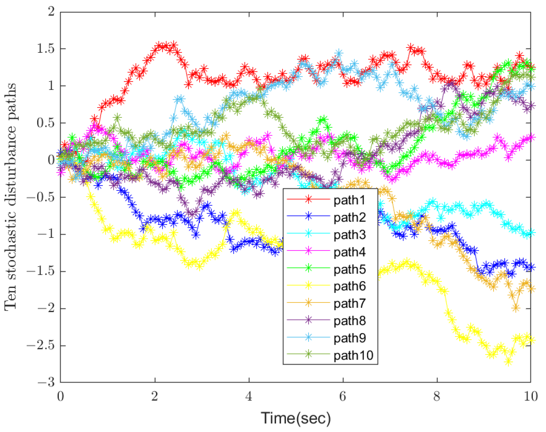Then the LQOC problem ${\mathfrak{E}}_i(i\in \{1,2,3,4\})$ in total could be indefinite. Thus the conditions of Theorem 2 are satisfied. We consider both random disturbance and discrete-time Markov chain in the modeling. The simulation results under the influence of 10 independent sets of disturbances and their average values are also presented. This comprehensive consideration enables the system to better simulate the uncertainty and dynamic changes in the real world and improves the robustness and adaptability of the system. In the existing research, few works can deal with these two complex factors at the same time, so it is significantly innovative in this respect. The initial condition is given by $x_0={[x_0^{11},x_0^{12},x_0^2]}^{\mathrm{T}}={[-1,1,0.02]}^{\mathrm{T}}$. The simulation results are given in Figure 1, Figure 2, Figure 3, Figure 4, Figure 5 and Figure 6.

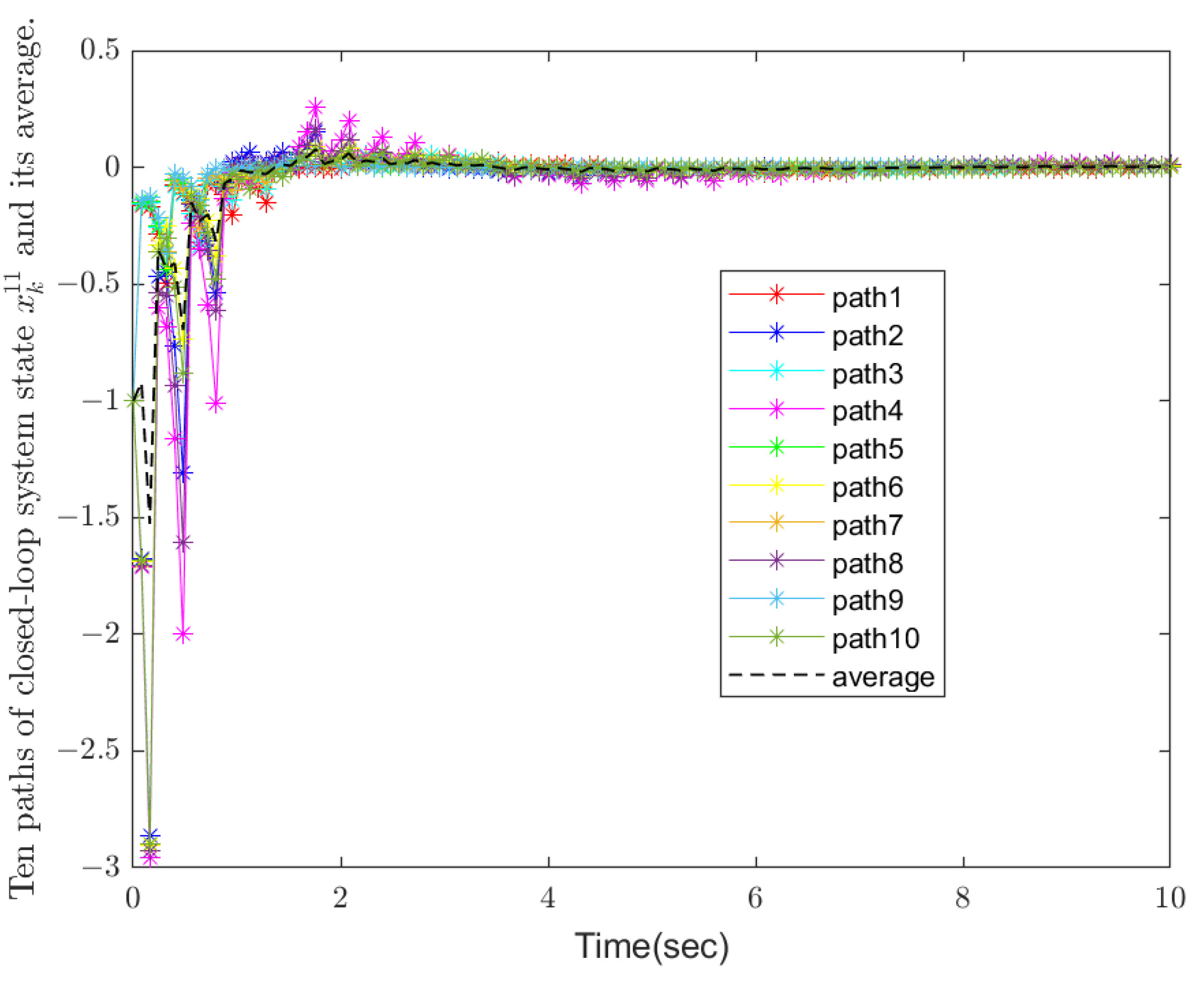
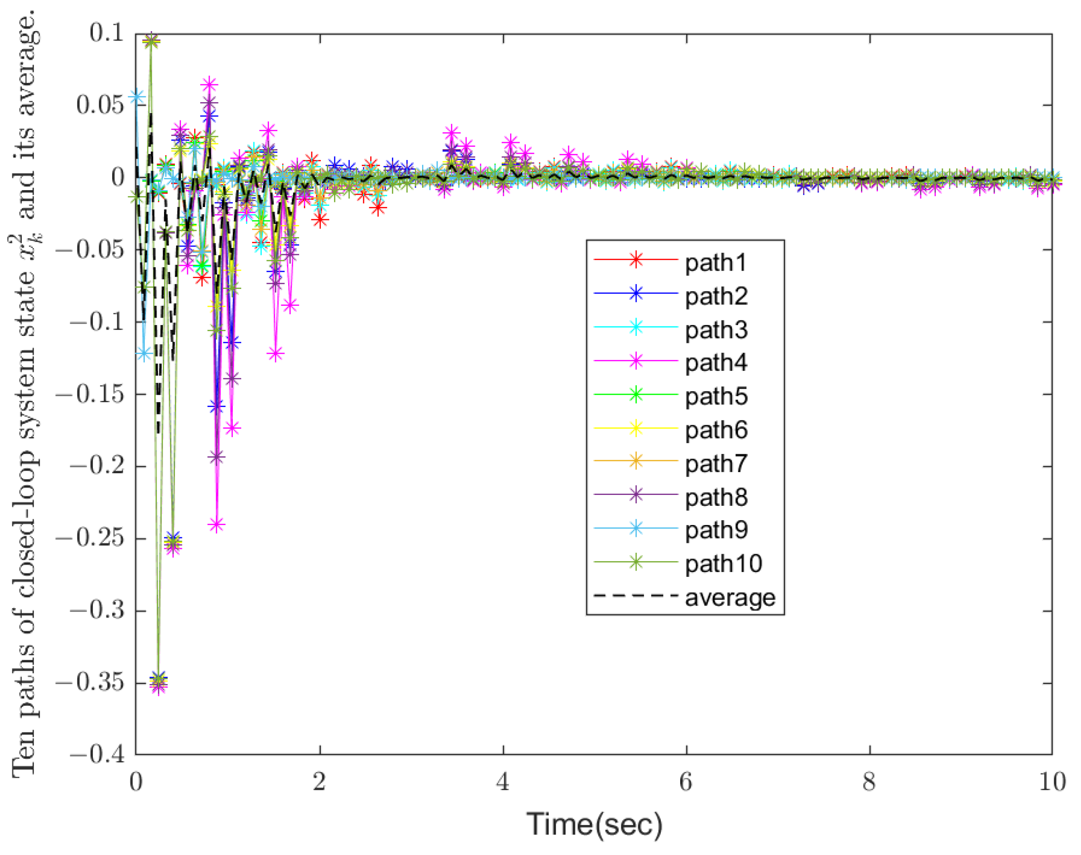
Figure 1 and Figure 2 show ten paths of stochastic disturbances and switching modes, respectively. It is easy to see that all the ten stochastic disturbances are independent and completely random, making the results more convincing and closer to real-world scenarios. Figure 3, Figure 4 and Figure 5 demonstrate the state trajectories $x_k^{11}$, $x_k^{12}$, and $x_k^2$ of the closed-loop systems along ten stochastic disturbances, while their average trajectories under ten samples are also shown, respectively. It indicates that each system state gradually smooths and tends to stabilize within a finite time. Then, Figure 6 shows control signals $u_k$, and it demonstrates that the designed controller is effective for the system. Finally, the optimal output feedback controller has been calculated by Theorem 2. Obviously, the figure shows that each of the 10 stochastic singular systems can reach stability and hold within $t=10$ under the influence of 10 independently generated stochastic disturbances, and the experimental simulation shows that the method has good results.

5. Conclusions

In conclusion, this study tackled the indefinite LQOC problem in discrete-time stochastic singular systems driven by stochastic disturbances and discrete-time Markov chains. This paper transformed the problem equivalently and proposed conditions for solvability, obtaining optimal control strategies and ensuring system regularity and causality. Definiteness conditions were established, yielding unique solutions for the GMJARE. This paper acquired optimal controls and nonnegative cost values to ensure system admissibility. And the related research conclusions are extended from the finite horizon to the infinite horizon. Output feedback controller design was presented using the LMI method, validated through illustrative examples. Future research could explore extensions to more complex system dynamics, investigate robustness to uncertainties, and consider practical implementation aspects for real-world applications. Additionally, incorporating machine learning techniques for adaptive control in stochastic environments could further enhance system performance and robustness.

References

1. Dai, L.Y. Singular Control Systems, Lecture Notes in Control and Information Sciences; Springer: Berlin, Germany, 1989. [Google Scholar]
2. Lam, J.; Xu, S.Y. Robust Control and Filtering of Singular Systems; Springer: Berlin, Germany, 2006. [Google Scholar]
3. Xia, Y.Q.; Zhang, J.H.; Boukas, E.K. Control for discrete singular hybrid systems. Automatica 2008, 44, 2635–2641. [Google Scholar] [CrossRef]
4. Yang, H.L.; Yang, L.J.; Ivanov, I.G. Reachable set estimation of discrete singular systems with time-varying delays and bounded peak inputs. Mathematics 2025, 13, 79. [Google Scholar] [CrossRef]
5. Chang, X.H.; Wang, X.Y.; Hou, L.W. New LMI approach to H control of discrete-time singular systems. Appl. Math. Comput. 2024, 474, 128703. [Google Scholar] [CrossRef]
6. Xu, Y.C.; Zhang, Y.J.; Zhang, J.F. Singularity-free adaptive control of discrete-time linear systems without prior knowledge of the high-frequency gain. Automatica 2024, 165, 111657. [Google Scholar] [CrossRef]
7. Wang, X.Y.; Zhang, Y.Q.; Yan, J.J.; Shi, Y. Event-triggered finite-time state estimation for discrete singular Markovian systems with quantization. J. Frankl. Inst. 2023, 360, 14430–14442. [Google Scholar] [CrossRef]
8. Han, Y.Y.; Zhou, S.S. Novel criteria of stochastic stability for discrete-time Markovian jump singular systems via supermartingale approach. IEEE Trans. Autom. Control 2022, 67, 6940–6947. [Google Scholar] [CrossRef]
9. Zhang, L.; Zong, G.D.; Zhao, X.D.; Zhao, N.; Sharaf, S. Reachable Set Control for Discrete-Time Takagi-Sugeno Fuzzy Singular Markov Jump System. IEEE Trans. Fuzzy Syst. 2023, 31, 3173–3184. [Google Scholar] [CrossRef]
10. Kao, Y.G.; Han, Y.Q.; Zhu, Y.Z.; Shu, Z. Stability analysis of delayed discrete singular piecewise homogeneous Markovian jump systems with unknown transition probabilities via sliding-mode approach. IEEE Trans. Autom. Control 2024, 69, 315–322. [Google Scholar] [CrossRef]
11. Zhang, Q.L.; Zhang, J.Y.; Wang, Y.Y. Sliding-mode control for singular Markovian jump systems with Brownian motion based on stochastic sliding mode surface. IEEE Trans. Syst. Man, Cybern. Syst. 2019, 49, 494–505. [Google Scholar] [CrossRef]
12. Zhou, H.; Hu, Y.Z.; Zhao, J.J. Numerical method for singular drift stochastic differential equation driven by fractional Brownian motion. J. Comput. Appl. Math. 2024, 447, 115902. [Google Scholar] [CrossRef]
13. Wang, S.Q.; Lian, G.G.; Cheng, C.; Chen, H.T. A novel method of rolling bearings fault diagnosis based on singular spectrum decomposition and optimized stochastic configuration network. Neurocomputing 2024, 574, 127278. [Google Scholar] [CrossRef]
14. Kalman, R.E. Contributions to the theory of optimal control. Bol. Soc. Mexicana 1960, 5, 102–119. [Google Scholar]
15. Elsisi, M.; Zaini, H.G.; Mahmoud, K.; Bergies, S.; Ghoneim, S.S.M. Improvement of trajectory tracking by robot manipulator based on a new co-operative optimization algorithm. Mathematics 2021, 9, 3231. [Google Scholar] [CrossRef]
16. Messerer, F.; Baumgartner, K.; Nurkanovic, A.; Diehl, M. Approximate propagation of normal distributions for stochastic optimal control of nonsmooth systems. Nonlinear Anal. Hybrid Syst. 2024, 53, 101499. [Google Scholar] [CrossRef]
17. Ferrante, A.; Ntogramatzidis, L. The generalized continuous algebraic Riccati equation and impulse-free continuous-time LQ optimal control. Automatica 2014, 50, 1176–1180. [Google Scholar] [CrossRef]
18. Ntogramatzidis, L.; Ferrante, A. On the solution of the Riccati differential equation arising from the LQ optimal control problem. Syst. Control Lett. 2010, 59, 114–121. [Google Scholar] [CrossRef]
19. Chávez-Fuentes, J.R.; Costa, E.F.; Terra, M.H.; Rocha, K.D.T. The linear quadratic optimal control problem for discrete-time Markov jump linear singular systems. Automatica 2021, 127, 109506. [Google Scholar] [CrossRef]
20. Li, Y.C.; Ma, S.P. Finite and infinite horizon indefinite linear quadratic optimal control for discrete-time singular Markov jump systems. J. Frankl. Inst. 2021, 358, 8993–9022. [Google Scholar] [CrossRef]
21. Lu, Q.Y.; Zhu, Y.G. LQ optimal control of fractional-order discrete-time uncertain systems. Chaos Solitons Fractals 2021, 147, 110984. [Google Scholar] [CrossRef]
22. Lu, Q.Y.; Zhu, Y.G.; Li, B. Necessary optimality conditions of fractional-order discrete uncertain optimal control problems. Eur. J. Control 2023, 69, 100723. [Google Scholar] [CrossRef]
23. Xu, M.Z.; Tang, M.N.; Meng, Q.X. Forward-backward stochastic evolution equations in infinite dimensions and application to LQ optimal control problems. Syst. Control. Lett. 2024, 185, 105748. [Google Scholar] [CrossRef]
24. Ye, L.W.; Zhao, Z.G.; Liu, F. Stochastic LQ optimal control for Markov jumping systems with multiplicative noise using reinforcement learning. Syst. Control Lett. 2024, 186, 105765. [Google Scholar] [CrossRef]
25. Wang, G.L.; Zhang, Q.L.; Yan, X.G. Analysis and Design of Singular Markovian Jump Sysytems; Springer: Cham, Switzerland, 2015. [Google Scholar]
26. Liu, X.K.; Li, Y.; Zhang, W.H. Stochastic linear quadratic optimal control with constraint for discrete-time systems. Appl. Math. Comput. 2014, 228, 264–270. [Google Scholar] [CrossRef]
27. Rami, M.A.; Chen, X.; Zhou, X.Y. Discrete-time indefinite LQ control with state and control dependent noises. J. Glob. Optim. 2002, 23, 245–265. [Google Scholar] [CrossRef]
28. Zhu, L.M.; Modares, H.; Peen, G.O.; Lewis, F.L.; Yue, B.Z. Adaptive suboptimal output-feedback control for linear systems using integral reinforcement learning. IEEE Trans. Control Syst. Technol. 2015, 23, 264–273. [Google Scholar] [CrossRef]
Figure 1. Ten stochastic disturbance paths.
Mathematics 13 00634 g001
Figure 2. Markovian switching modes.
Mathematics 13 00634 g002
Figure 3. State trajectories x k 11 of the closed-loop model.
Mathematics 13 00634 g003
Figure 4. State trajectories x k 12 of the closed-loop model.
Mathematics 13 00634 g004
Figure 5. State trajectories x k 2 of the closed-loop model.
Mathematics 13 00634 g005
Figure 6. System control signal u k .
Mathematics 13 00634 g006
Disclaimer/Publisher’s Note: The statements, opinions and data contained in all publications are solely those of the individual author(s) and contributor(s) and not of MDPI and/or the editor(s). MDPI and/or the editor(s) disclaim responsibility for any injury to people or property resulting from any ideas, methods, instructions or products referred to in the content.