Abstract
Motor impairment is a critical health issue that restricts disabled people from living their lives normally and with comfort. Detecting motor imagery (MI) in electroencephalography (EEG) signals can make their lives easier. There has been a lot of work on detecting two or four different MI movements, which include bilateral, contralateral, and unilateral upper limb movements. However, there is little research on the challenging problem of detecting more than four motor imagery tasks and unilateral lower limb movements. As a solution to this problem, a spectral-spatio-temporal multiscale network (SSTMNet) has been introduced to detect six imagery tasks. It first performs a spectral analysis of an EEG trial and attends to the salient brain waves (rhythms) using an attention mechanism. Then, the temporal dependency across the entire EEG trial is worked out using a temporal dependency block, resulting in spectral-spatio-temporal features, which are passed to a multiscale block to learn multiscale spectral-–spatio-temporal features. Finally, these features are deeply analyzed by a sequential block to extract high-level features, which are used to detect an MI task. In addition, to deal with the small dataset problem for each MI task, the researchers introduce a data augmentation technique based on Fourier transform, which generates new EEG trials from EEG signals belonging to the same class in the frequency domain, with the idea that the coefficients of the same frequencies must be fused, ensuring label-preserving trials. SSTMNet is thoroughly evaluated on a public-domain benchmark dataset; it achieves an accuracy of 77.52% and an F1-score of 56.19%. t-SNE plots, confusion matrices, and ROC curves are presented, which show the effectiveness of SSTMNet. Furthermore, when it is trained on augmented data generated by the proposed data augmentation method, it results in a better performance, which validates the effectiveness of the proposed technique. The results indicate that its performance is comparable with the state-of-the-art methods. An analysis of the features learned by the model reveals that the block architectural design aids the model in distinguishing between multi-imagery tasks.
Keywords:
brain–computer interface (BCI); EEG brain signal; motor imagery (MI); attention; multiscale; deep learning; convolutional neural network; Gated Recurrent Unit (GRU) MSC:
68T07
1. Introduction
Motor impairment is a critical disability that occurs when motor limbs lose their main movement role due to different reasons [1,2]. At any stage of their lives, people can be affected by short-term or long-term motor disabilities, meaning they cannot practice normal daily routines and activities due to mobility deficits. This has raised the need for communication methods to enable people with motor disabilities to easily interact with their surrounding environment and enhance the quality of their lives. The brain–computer interface (BCI) is one of the communication methods that enables users to interact and control external environments without muscle activity by decoding messages and commands directly with brain signals [3,4,5]. A commonly used non-invasive technique to capture brain activations is electroencephalography (EEG) [6]. Its high temporal resolution, affordable price, and ease of use make EEG a favorable choice for BCI applications [7]. EEG-based motor imagery has become prominent in EEG-based BCI applications and research domains. Many studies have taken advantage of EEG-based MI to address problems related to the control and rehabilitation process [8,9].
The main problem in MI detection is decoding messages and commands from an EEG signal, and different traditional machine learning [10,11] and deep learning [12,13,14] techniques have been proposed to solve this problem. The notable traditional machine learning techniques are based on a common spatial pattern (CSP) in combination with local activity estimation (LAE), Mahalanobis distance, and support vector machines (SVMs) [15,16]. The most representative deep learning models that have been widely used for decoding MI tasks are EEGNet [17], shallow, and DeepNet [18]. Most works based on traditional machine learning and deep learning focus on a small number of MI tasks ranging from two to four. Additionally, MI tasks involve bilateral, contralateral, and unilateral movements of the upper limbs. However, the problem becomes challenging when the number of MI tasks is greater than four and involves unilateral motor imagery, such as the left hand, right hand, left leg, and right leg. There are a few research works that have addressed more than four MI tasks [10,11,13]. These works build solutions based mainly on existing traditional machine learning techniques and deep learning models. This necessitates the development of custom-designed techniques. In view of this, a custom-designed solution has been proposed for this problem, leveraging the spectral and multiscale nature of EEG trials, and in this paper specifically, a deep learning model has been introduced that utilizes attention and sequential modeling techniques, along with CNN layers.
An EEG signal is composed of various brain waves (rhythms or frequency bands) such as delta (0.5–4 Hz), theta (4.0–7.0 Hz), alpha (8.0–12.0 Hz), beta (12.0–30.0 Hz), and gamma (30.00–50.0 Hz) [19]. These brain waves play a key role in decoding motor imagery events from EEG brain signals [7,19]. The MI triggers changes in the brain waves corresponding to a subject’s intent movements. These changes help to discriminate various MI tasks, which eventually causes an MI BCI system to detect MI tasks and interpret them to assist disabled people in interacting with the environment [3,4,5]. However, the existing MI detection methods do not adequately focus on analyzing brain waves and extracting spectral information from EEG trials. Further, the multibranch temporal analysis of an EEG signal [14] and long-term temporal dependencies also play an important role in discriminating MI tasks [14]. Based on these observations, the SSTMNet has been proposed to detect MI tasks. Specifically, the main contributions of this work are as follows:
- A spectral–spatio-temporal multiscale deep network—SSTMNet—that first performs a spectral analysis of an input EEG trial by decomposing each channel into brain waves, paying due attention relevant to an MI task to each brain wave, then working out long-term temporal dependencies and performing a multiscale analysis; finally, it performs a deep analysis to extract high-level spectral–spatio-temporal multiscale features and classifies the trial.
- A data augmentation technique to deal with the small dataset problem for each MI task. It generates new EEG trials from EEG signals belonging to the same class in the frequency domain with the idea that the coefficients of the same frequencies must be fused, ensuring label-preserving trials.
- The effect of the data augmentation technique and the performance of SSTMNet for unilateral MI tasks on the benchmark public-domain dataset are thoroughly evaluated and compared with similar state-of-the-art methods.
- A qualitative analysis of the discriminatory potential of the features learned by the SSTMNet and its decision-making mechanism is presented.
The remaining sections are organized as follows: Section 2 presents an overview of the most relevant state-of-the-art works on EEG-based MI detection. The proposed method is explained in Section 3. The details of the evaluation protocol, the description of the dataset, and data augmentation are provided in Section 4. The experimental results and discussion are described in Section 5 and Section 6, respectively. Finally, Section 7 concludes the paper.
2. Related Works
The problem of decoding MI tasks from EEG signals has been under consideration since the 1990s [20]. The detection of motor imagery patterns in EEG signals is rapidly progressing using conventional machine learning and deep learning techniques. This section reviews the representative works on MI task detection using EEG signals. A summary of the comparison between various methods is presented in Table 1.
Most published works have addressed from two to four motor imagery classes and were evaluated using many benchmark datasets developed for these tasks [21,22,23]. Regarding more than four MI tasks, there are few studies as well as the benchmark datasets [24,25,26,27]. Ofner et al. [25] focused on six MI tasks associated with the right upper limbs (elbow, forearm, and hand) and rest state. Yie et al. [26] developed a dataset that involves six simple and compound MI tasks related to the hands and legs. Jeong et al. [27] developed a dataset that contains eleven MI tasks specific to the same upper limb, including arm-reaching, hand-grasping, and wrist-twisting. Kaya et al. [24] built a large MI dataset that involves five fingers, hands, legs, tongue, and a passive state. It is divided into the following three paradigms: five fingers (5F), hands/legs/tongue and passive (HaLT), and hands and passive state (CLA). Most studies focus on unilateral and contralateral MI tasks for the upper body parts. However, Kaya et al.’s [24] dataset focused on unilateral MI tasks for the hands and legs; they also introduced challenging MI tasks involving using one finger at a time.

Table 1.
Summary comparison of literature reviews between dataset, number of subjects (#Sub), method, number of channels (#Ch), and number of MI tasks (#MI Tasks).
Table 1.
Summary comparison of literature reviews between dataset, number of subjects (#Sub), method, number of channels (#Ch), and number of MI tasks (#MI Tasks).
| References | Dataset | # Sub | Method | # Ch | # MI Tasks | Acc. |
|---|---|---|---|---|---|---|
| Lian et al., (2024) [12] | Private | 10 | CNN + GRU + Attention | 34 | Six Tasks (RH, LH, both hands, both feet, right arm + left leg, and left arm + right leg) | 64.40% |
| Wirawan et al., (2024) [28] | MIMED | 30 | SVM + baseline reduction | 14 | Raising RH, lowering RH, raising LH, lowering LH, standing, and sitting | 83.23% |
| George et al., (2022) [13] | HaLT [24] | DeepNet | 19 | LH, RH, Passive state, LL, Tongue, RL | 81.74–83.01% | |
| George et al., (2022) [14] | DeepNet | - | 81.49% | |||
| George et al. [29]-2022 | 12 | Multi-Shallow Net | - | 81.92% | ||
| Mwata-Velu et al., (2023) [30] | EEGNet | 8–6 | 83.79% | |||
| Yan et al., (2022) [31] | Graph CNN + Attention | 19 | 81.61% | |||
| Yang et al., (2024) [10] | 5F [24] | 8 | Features selection + Feature fusion + Ensemble learning (SVM, RF, NB) | 22 | 5 Fingers | 50.64% |
| Degirmenci et al., (2024) [11] | NoMT + 5F [24] | 13 | Intrinsic Time-Scale Decomposition (ITD) + Ensemble Learning | 19 | 5 Fingers + Passive state | 55% |
A few studies focused on six MI tasks. Lian et al. [12] proposed a hybrid DL model to extract spectral and temporal features. It consists of four stacked CNN layers and two GRU layers, followed by an attention technique to reweight the extracted features. The evaluation was carried out on a private dataset that involved six MI tasks performed by ten healthy subjects, yielding an accuracy of 64.40%. Wirawan et al. [28] developed a motor execution (ME) and imagery (MI) dataset for six motor tasks related to different hand positions, as well as standing and sitting movements. They preprocessed an EEG trial using different methods, such as separating a baseline signal from the trial, normalization, and frequency decomposition. Then, they extracted features using differential entropy and used baseline reduction to overcome inferences in a trial. Finally, they used decision trees and SVM to assess the baseline reduction process in recognizing motor patterns. The results showed that SVM with a baseline reduction approach achieved an 83.23% accuracy.
George et al. [13] employed DeepNet and examined different data augmentation methods on the HaLT paradigm [24]. The accuracy ranged between 81.74% and 83.01% compared to no DA 80.73%. George et al. [14] employed Bi-GRU, DeepNet, and Multi-Branch Shallow Net to classify MI tasks in the HaLT paradigm; they used within- and cross-subject transfer learning approaches, in addition to the subject-specific approach for evaluation. The subject-specific evaluation resulted in a better performance (Bi-GRU 77.70 ± 11.06, DeepNet 81.49 ± 11.43, and Multi-Shallow Net 78.32 ± 7.53). George et al. [29] also conducted a study comparing the performances of traditional methods, existing deep learning models, and their combinations in classifying MI tasks in the HaLT paradigm. Deep learning models showed superior results over conventional methods. The highest accuracy achieved among all experiments was 81.92 ± 6.48 using Multi-Shallow Net. Mwata-Velu et al. [30] used EEGNet and introduced two channel selection methods based on channel-wise accuracy and mutual information. They evaluated their methods using the subject-independent protocol with 10-fold cross-validation in the HaLT paradigm; the study reached an accuracy of 83.79%. Yan et al. [31] employed a graph CNN with an attention mechanism, and the EEG signal was reshaped into two graph representations, spatial–temporal and spatial–spectral. The two representations were fed into the model in parallel and then their features were fused. A subject-specific protocol with a 5-fold CV was used to classify the HaLT paradigm, achieving an accuracy of 81.61%.
Some studies focused on classifying five MI tasks [10,11]. Yang et al. [10] proposed a method for evaluating and selecting EEG signal sub-bands in two stages. Firstly, bands were identified with high correlation coefficients between features and labels, and then their effectiveness was verified by computing their average accuracy using SVM, Random Forests, and Naive Bayes. Then, Fourier transform amplitudes and Riemannian geometry were used to extract features, followed by a feature selection process. Finally, ensemble learning was applied through weight voting. They achieved an average accuracy of 50.64 ± 10.88 in classifying five fingers (5F paradigm). Degirmenci et al. [11] proposed a novel feature extraction method by decomposing EEG signals using the intrinsic time-scale method and selecting the first three high-frequency components (PCRs) for further analysis. Various features such as power, mean, and sample entropy were extracted from individual PCRs and their combinations and analyzed using the feature selection method. Well-known machine learning classifiers were utilized to classify selected features, and the performance of the ensemble learning classifier was the best. The study combined the NoMT and 5F paradigms in [24] to classify six classes, and the accuracy ranged from 35.83 to 55% using a subject-dependent protocol.
The studies in [12,28] focused on a large number of MI tasks, most of which were bilateral and contralateral MI movements, and unilateral MI was evaluated only for hands. In [12], trials were recorded through 34 channels distributed over the skull, leading to interference and redundancy in the recorded signals. In [28], the reported accuracy was on a motor execution dataset rather than motor imagery. Some studies employed existing deep learning models such as DeepNet and EEGNet [13,14,29,30]. Additionally, the studies in [13,29] used many preprocessing techniques such as bandpass filter, baseline correction, artifact correction, data re-referencing, and trial rejection process.
A few studies focused on more than four MI tasks and employed existing deep learning models or traditional machine learning algorithms. As these studies employed existing techniques, they did not deeply analyze the spectral information and multiscale content of an EEG signal and yielded a poor performance. Further research is needed to overcome the limitations of the existing methods.
3. Proposed Methods
In this section, the problem is first formulated, and then the details of the proposed deep learning-based model are presented.
3.1. Mathematical Formulation of the Problem
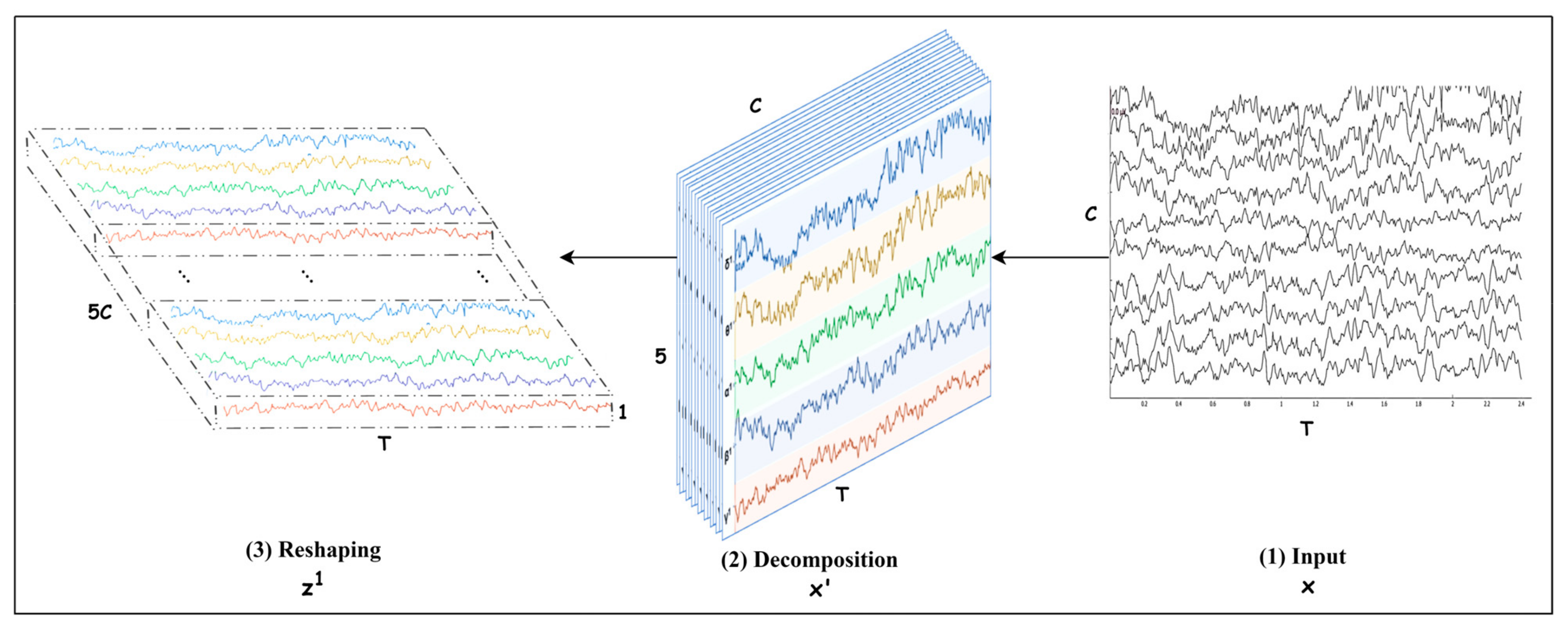
The problem is identifying the motor imagery (MI) class from an EEG trial. An EEG trial consists of channels captured with electrodes placed on the skull during seconds. If the sampling rate is , then the number of samples in each channel is . Let us denote a trial with , then , as shown in Figure 1. Each channel is decomposed into five frequency bands (brain waves) , and then is transformed into where is the number of frequency bands. Further, the bands are stacked in such a way that takes the form where =, as depicted in Figure 1. This representation helps to identify the channel and the frequency bands that play a key role in decoding an MI class. The trial can also be expressed as a time series [, where The details for preprocessing an EEG trial and transforming it into are discussed in Section 3.2.
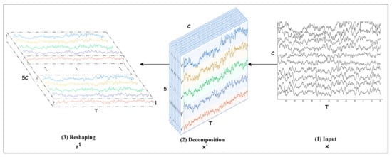
Figure 1.
Spectral decomposition and reshaping.
Let there be six imagery classes, and Y = {left hand, right hand, passive state, left leg, tongue, right leg} is the set of labels of these classes. To identify the MI class of a trial , a mapping needs to be built, which takes a trial as input and yields its class as an output, i.e., , where are parameters of the mapping . Because of the outstanding performance of deep learning in various applications, using a deep learning-based model is designed, which allows end-to-end learning. Section 3.3 introduces the details of the proposed deep learning-based model for
3.2. Preprocessing
This section introduces the preprocessing methods that are applied on the trial . Firstly, the trial is standardized using a local channel standardization method. Afterward, it is transformed from to by the spectral decomposition process.
3.2.1. Local Channel Standardization
The EEG trial is standardized locally. Then, the mean and standard deviation σi are computed for each channel of , i.e.,
Using and , each channel is standardized as follows:
It helps to handle the outliers in each channel independently and unify the mean to be zero and the standard deviation to equal one, which introduces consistency among channels.
3.2.2. Spectral Decomposition
An EEG signal consists of various frequency bands (brain waves), including delta (0.5–4 Hz), theta (4.0–7.0 Hz), alpha (8.0–12.0 Hz), beta (12.0–30.0 Hz), and gamma (30.00–50.0 Hz) [19]. These frequency bands are crucial for decoding motor imagery (MI) events from EEG brain signals [7,19]. MI induces changes in the frequency bands related to a subject’s intended movements. These changes help to distinguish various MI tasks, enabling an MI brain–computer interface (BCI) system to detect and interpret MI tasks, assisting disabled individuals in interacting with their environment [3,4,5]. This indicates that spectral information must be extracted from each channel of an EEG signal by decomposing it into frequency bands.
Due to the temporal localization of 1D discrete wavelet transform (DWT), in this work, DWT is used to decompose the standardized EEG trial into five frequency bands and transform it to . This process is conducted using DWT in PyWavlets package [32] and Daubechies-4 (db4) [33]. Each EEG channel is decomposed into an approximation coefficient A5 and detail coefficients D1, D2, D3, D4, and D5 using five levels of decomposition based on the following equation [33]:
where is the sampling rate and [ is the frequency band at level l. The detail coefficient D1 is noise and A5, D2, D3, D4, and D5 represent delta, theta, alpha, beta, and gamma bands, respectively.
3.3. Proposed Model
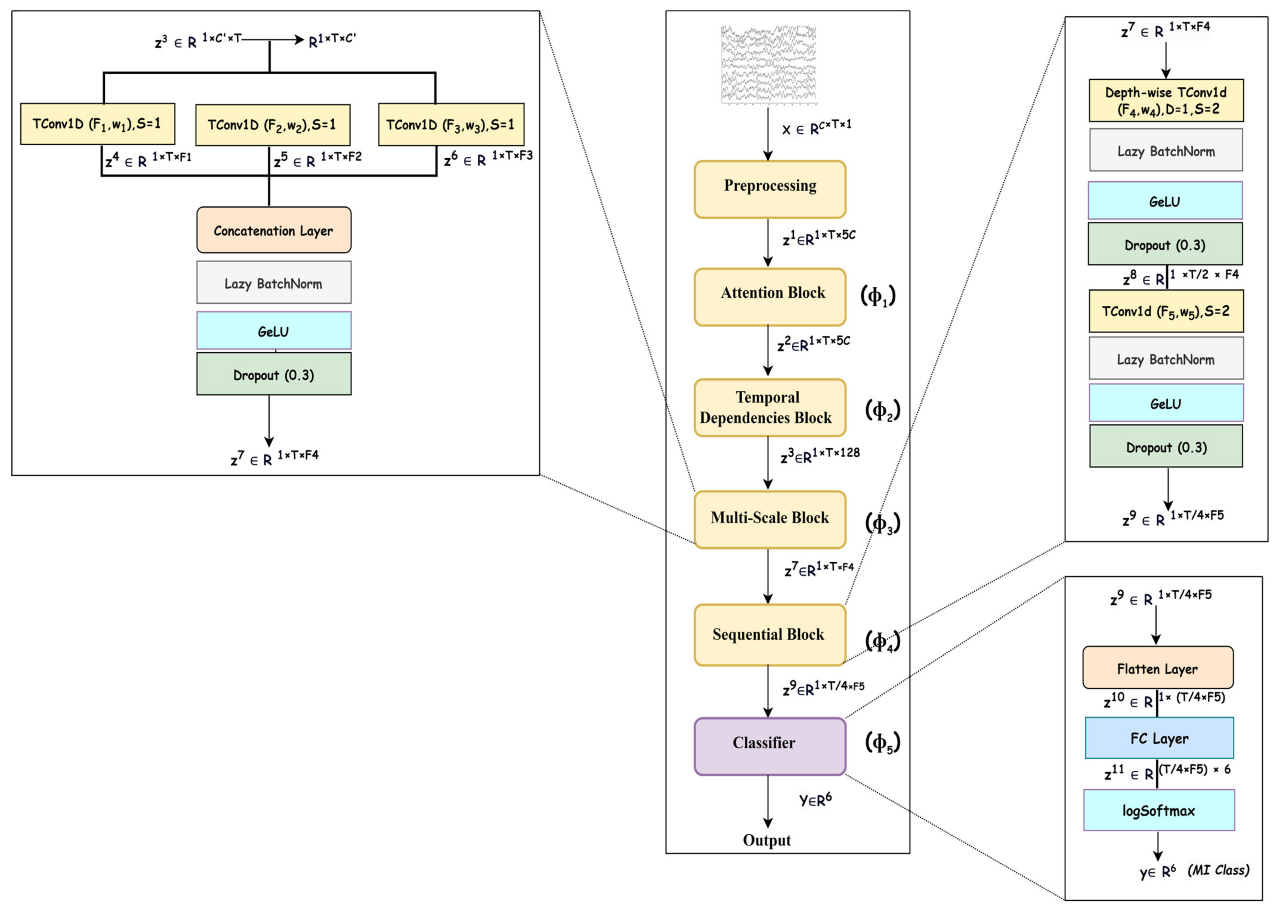
An overview of the deep neural network designed for modeling is shown in Figure 2, and it consists of five blocks that represent f as a composition of five mappings, i.e., , where represents the learnable parameters of all mappings; the details of each mapping are given in the upcoming subsections. As the mappings learn spectral–spatio-temporal and multiscale features, the network SSTMNet is used in the onward discussion.

Figure 2.
Overview of spectral–spatio-temporal multiscale network (SSTMNet).
An EEG trial is captured using electrodes as a signal consisting of channels, which record brain activation due to cognitive tasks in various brain lobes [34]. As MI induces changes in the frequency bands related to a subject’s intended movements, this emphasizes that an EEG trial must be decomposed into frequency bands to extract spectral information from each channel, and attention must be paid to each frequency band depending on its relevance to the MI task. For this reason, the attention block () is utilized to elicit and suppress frequency bands depending on their importance to the motor imagery task. Due to the same reason, this is followed by a temporal dependencies block () to work out the long-range dependencies in the channel and time dimensions of the time series data and extract the spatio-temporal features. This is similar to the source separation of independent component analysis (ICA) [35], but it is more robust because it automatically learns the interaction between signals originating from different lobes at different times, taking into account the temporal and channel dimensions. Furthermore, an EEG signal is composed of features at different scales, and it is necessary to extract discriminative representation through a multiscale signal analysis. Multiscale analysis helps to overcome inter- and intra-subject variability [36]. The multiscale block ( performs multiscale analysis in the temporal dimension to extract multiscale features. Finally, the sequential block () learns high-level features relevant to a specific MI task, which are passed to the classification block () for inference. The details of the architecture are presented in Table 2.
Table 2.
Proposed method architecture including kernel size/Number of filters (#Filters), stride, output, and number of parameters (# Param).
3.3.1. Attention Block
Conducting cognitive tasks triggers multiple brain regions, leading to interaction and information flow between these regions. In addition, the ERS/ERD phenomena in ongoing EEG signals complicate the feature extraction process, because they occur at multiple brain regions, frequencies, and time spans [34]. Focusing on the frequency bands that play crucial roles in MI task detection is essential. For this purpose, each channel of the input EEG trial is decomposed into five frequency bands, producing a multichannel signal , where each channel corresponds to a frequency band. We then apply mapping one to recalibrate to that pays more attention to the salient bands.
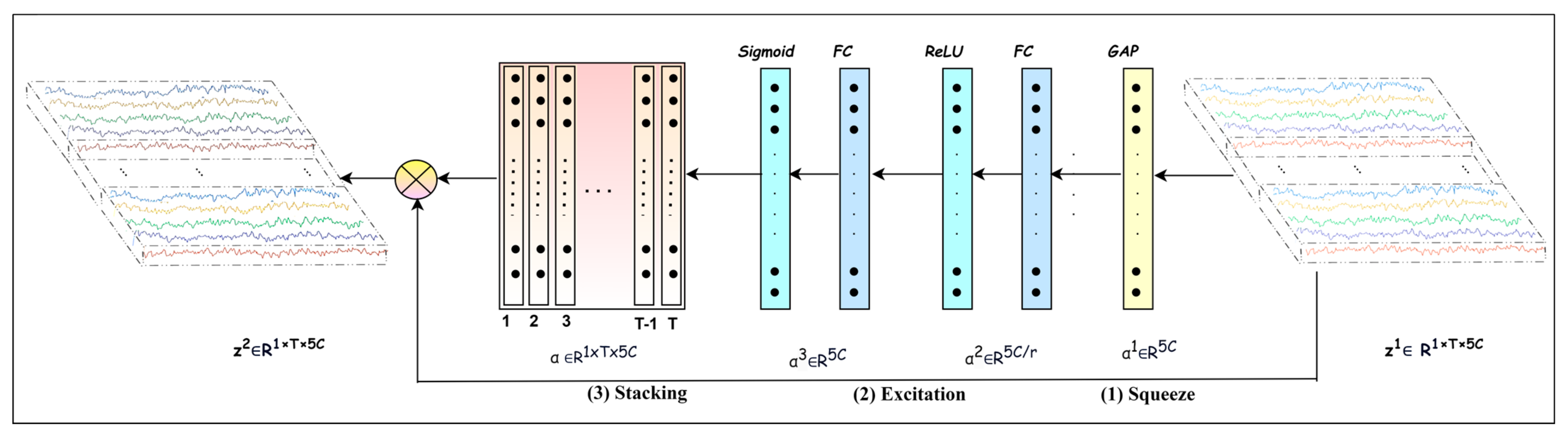
The is built using the attention mechanism introduced in [37], which helps to recalibrate to elicit the discriminative channels and suppress the less discriminative ones, thereby emphasizing effective frequency bands relevant to an MI task. The mapping is composed of different functions, as follows:
where
It is composed of the following three operations: squeeze, excitation, and recalibration. Equation (5) computes the recalibration coefficients using squeeze (Equations (7) and (8)), excitation (Equations (9) and (10)), and stacking operations. In the squeeze operation, applies global average pooling across the temporal dimension, as illustrated in Equations (7) and (8). By computing the average along the temporal dimension of , it shrinks to one statistical descriptor. The excitation operation further analyzes the independent descriptors corresponding to 5C bands to learn the interdependencies between bands and generate the recalibration coefficients representing the importance of each of the bands.
Referring to Figure 3, the excitation operation is implemented using two fully connected layers followed by activation layers. The vector of descriptors is fed into the first fully connected layer followed by activation to reduce its dimension from to and yield The second fully connected layer is followed by activation, and it enlarges its dimension back to generating . In this way, the excitation operation learns the interdependencies among bands. The reduction ratio is selected by experiments, and it is found that r = 10 produced a good performance. Furthermore, this operation using non-linear activation and introduces nonlinearity and ends up with the recalibration coefficients as probability values representing the importance level of each band. Finally, a recalibrated trial is obtained by applying element-wise multiplication between the stacked recalibration coefficients and the input . The objective is to explore salient frequency bands to help the upcoming blocks to extract effective features.
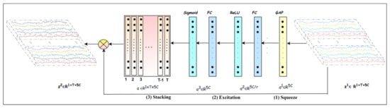
Figure 3.
Attention block.
3.3.2. Temporal Dependencies Block
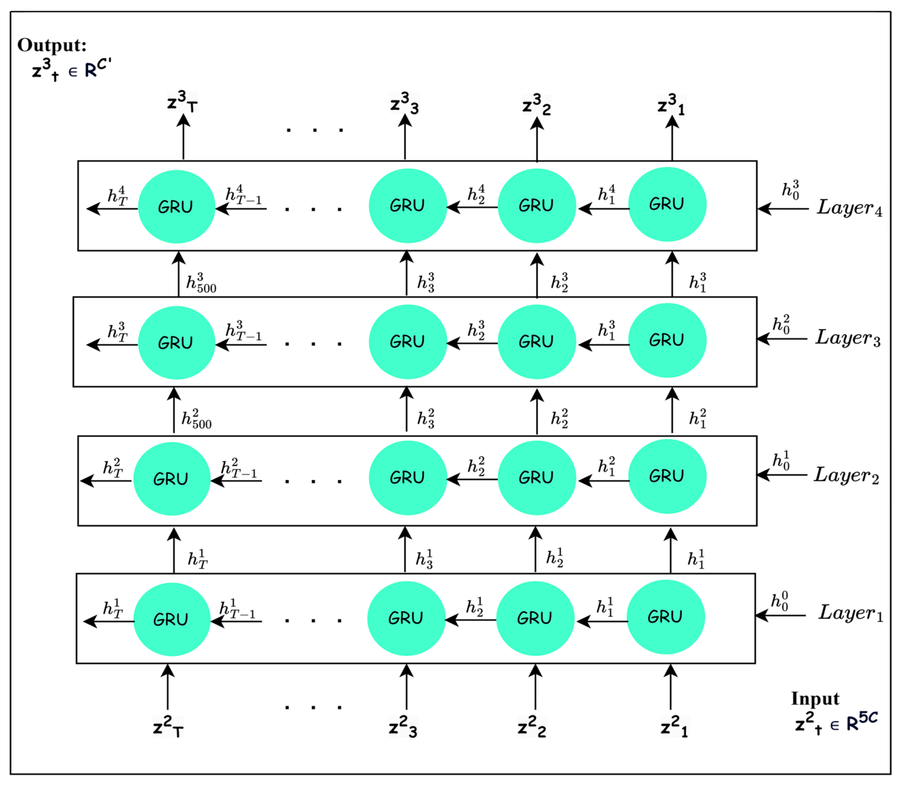
To learn discriminative features, it is important to consider the long-range temporal dependencies between frequency bands after their recalibration. The mapping works out the long-range temporal dependencies. The most sophisticated recurrent neural network architectures, such as LSTM and GRU, have achieved considerable improvements in different fields due to their ability to learn long-term dependencies [38]. Based on the results in [39], the superiority between GRU and LSTM cannot be specified. Several experiments are conducted to demonstrate that GRU is superior to LSTM in the proposed architecture. Thus, as GRU is able to maintain short-term and long-term dependencies [40], is implemented using a GRU block, as shown in Figure 4. For learning deep features with long-range dependencies, four GRU layers are stacked, as depicted in Figure 4, to define mapping , where each layer performs the following operations:
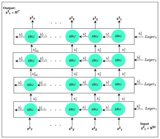
Figure 4.
The typical structure of GRU layers (temporal dependencies block).
The recalibrated signal is reshaped into to be compatible with the input to GRU block. Each GRU layer in the GRU block processes the input information from the current time and previous times using two gates, as explained in Equations (11)–(14) [40].
Firstly, the reset gate trains learnable parameters and to control the amount of insignificant information that should be neglected based on the input and previous hidden state [38,40]. It calculates probability values through the sigmoid function ( to discard insignificant information in the previous hidden state that is included with the reweighted input in computing the candidate value [38,39,40], as shown in Equation (13). Thus, the candidate value includes the high-level features originating from the input and new features that are created from the unforgotten part of the previous hidden state added to the reweighted input .
Secondly, the update gate manages the amount of significant information that should be preserved from as depicted in Equation (12) [38,39,40]. Finally, the weighted features in the hidden state are obtained using linear interpolation between the previous hidden state and current candidate [38,39,40].
The GRU layers are stacked in such a way that the output , I = 1, 2, 3 of the ith GRU is passed to the (i + 1)th layer. The number of GRU layers and the hidden-state features are chosen based on experiments. By stacking four GRU layers, the output is obtained, which contains deep high-level features computed considering the long-range temporal dependencies among the frequency bands.
3.3.3. Multiscale Block
A close look at an EEG signal reveals that features are found at multiple scales due to intra-subject and inter-subject variabilities, and analyzing them using fixed-size convolutional filters will not be able to handle subjects and time variabilities and hinder the extraction of different scales of features [36]. Inspired by this observation, high-level features are analyzed at different scales using multiscale convolutions similar to the naïve inception module [41].
The output from the temporal dependencies block is , which is reshaped from to to be suitable for 1D convolutional layers. Then, the mapping is , which is applied to extract multiscale features. This mapping takes the input and uses three temporal convolutional layers with F1, F2, and F3 filters with sizes of w1, w2, and w3, respectively, to yield multiscale features , and as follows:
As the filter sizes of the temporal convolutional layers are different, they learn multiscale spectral–spatio-temporal features from the high-level spectral–spatio-temporal features . It is found that , , and 25 and F1 = 32, F2 = 32, and F3 = 64 result in deep salient features related to MI tasks. Then, the features , and are concatenated across the channel dimension using a concatenation layer to generate the multiscale features , where . Then, batch normalization is applied with Lazy initialization ( and GeLU activation ( to produce the final features , as shown in Figure 2. Formally, the mapping is defined as follows:
Note that a dropout layer is employed with a dropout rate of 0.3 after the GeLU layer as a regularization layer to avoid overfitting during training. The Optuna package [42] is used in this work to effectively select the best normalization layer, activation function, and dropout value.
3.3.4. Sequential Block
The mapping is applied to learn higher-level multiscale spectral–spatio-temporal features from the output of the multiscale block. To keep the complexity of the model low, this mapping employs one depth-wise convolution layer [43] and one convolution layer, (see Figure 2) as follows:
The depth-wise temporal convolution layer ( is used with a filter size of and number of filters equal to , where . Also, uses a stride of 2 along the temporal dimension to compress the feature maps to half their original size, i.e., T/2. As a result, this reduces the model complexity.
Then, a temporal convolution layer ( is employed to extract compressed higher-level multiscale spectral–spatio-temporal features, as follows:
The layer uses filters of the size and a stride equal to 2, which further downsamples the input feature maps by the ratio of 2 along each dimension. This means that the feature maps are compressed by ratios of 4 and 2 along the time and channel dimensions, respectively, after this operation, which significantly reduces the complexity of the model and helps to avoid overfitting. Note that both convolutional layers are followed by lazy batch normalization (, GeLU activation ( and dropout to enhance the features extraction process. Finally, the mapping is composed of , as follows:
3.3.5. Classification Block
Finally, the mapping takes the learned multiscale spectral–spatio-temporal features and predicts the MI class of the input EEG trial. It first applies the flatten layer ( and one fully connected layer ( with n neurons, where n is the number of MI classes, followed by logSoftmax layer , i.e.,
where is the vector of posterior probabilities, and y is the label of the predicted class, such that
4. Evaluation Procedure
This section presents the evaluation procedure that followed to evaluate the performance of SSTMNet. It also gives a description of the public-domain benchmark EEG MI dataset [24] and performance metrics used to assess SSTMNet’s performance. Finally, the data augmentation method that was applied to the dataset is introduced in detail.
SSTMNet was implemented using Python version 3.10.12, and the experiments were conducted on Google Colab Pro+ equipped with a Tesla T4 GPU and 15 GB RAM. In this section, a detailed description of the training procedure is also provided.
4.1. Dataset Description and Preparation
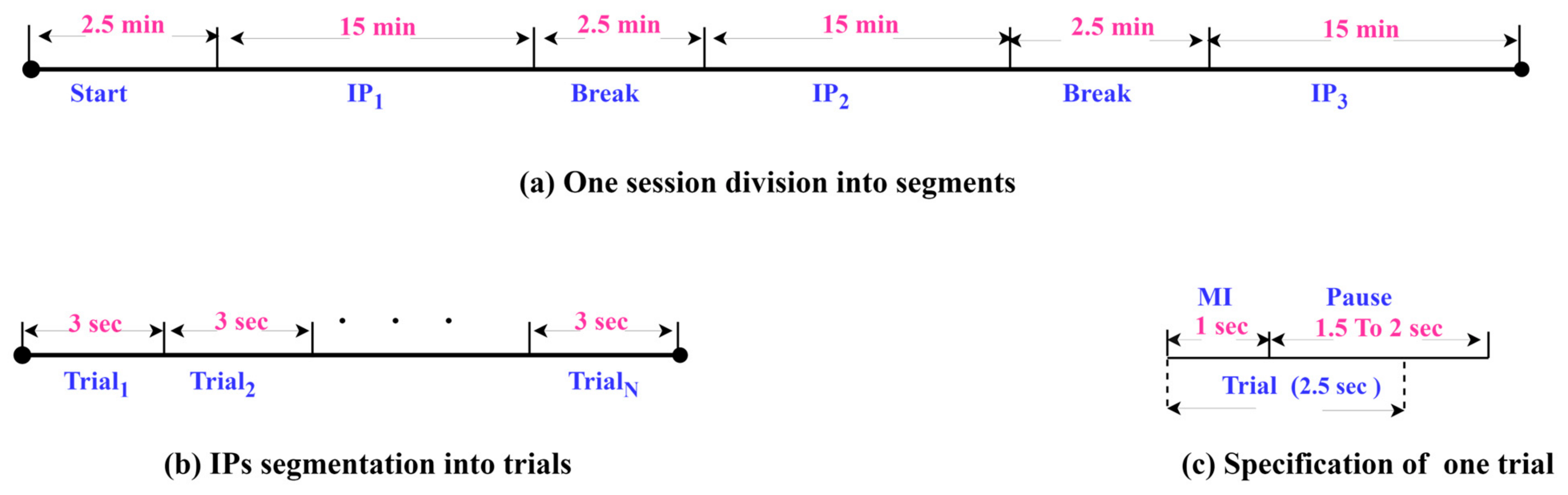
SSTMNet has been tested on a public-domain benchmark EEG MI dataset [24] which involves three paradigms. This work is mainly focused on the HaLT paradigm, which stands for hands, legs, and tongue; it involves MI tasks, i.e., left- and right-hand, left- and right-leg, passive, and tongue imaged movements. Twelve healthy subjects participated in this paradigm labeled from ‘A’ to ‘M’, excluding the letter ‘D’. The number of sessions varied from 1 to 3 for each subject, resulting in a final production of 29 files. The duration of sessions ranged from 50 to 55 min. Each session was divided into interaction periods (IPs); it started with 2.5 min as an initial relaxation, and then the IPs were separated with 2.5 min (as depicted in Figure 5a). In each IP segment, a subject performed 300 trials, and each trial took 1 s for the MI task and 1.5 s to 2 s as a pause, as shown in Figure 5b. The EEG-1200 system with Neurofax software was used to record the 19-channel EEG signals at a sampling rate of 200 Hz; and were recorded as ground channels and as a bipolar channel for synchronization purposes. The 10/20 international system was adopted to position the electrodes over the scalp. Due to the use of the EEG-1200 system and Neurofax software, two hardware filters were applied to the recorded data, a notch filter (50 Hz) and bandpass filters (0.53–70 Hz).
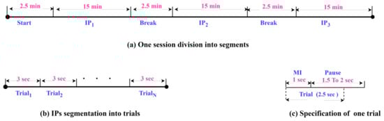
Figure 5.
The details of dataset sessions and segmentation.
For the experiments, EEG trials of 2.5 s were extracted, as shown in Figure 5c. Each trial involved 1 s for MI task and 1.5 s of the pause period to ensure that the entire motor imagery signal was captured due to the continuity of the thought process after 1 s.
4.2. Dataset Augmentation
On average, each subject and class had a set of 159 EEG trials, which is insufficient to train even a lightweight deep network. To tackle the small dataset problem, a data augmentation method was proposed to create new EEG trials from the existing EEG trials in the frequency domain. The idea is that trials belonging to the same class share similar patterns in the frequency domain, and the coefficients of the same frequencies must be interpolated to ensure the creation of new label-preserving trials.
A trial in a time domain is transformed into a frequency domain using DFT [44] as follows:
where are the frequency coefficients.
Two different trials from the same class, , are selected, where , and is the total number of trials of the class. are transformed to using Fast Fourier Transform (FFT). The new trial is created by interpolation in the frequency domain, as follows:
The new trial is in the frequency domain. It is transformed to the time domain using inverse Fast Fourier transform (IFFT), as follows:
Please note that the new trial is created by interpolating the corresponding frequency coefficients. This interpolation ensures that the new trial has the same label as , i.e., the data augmentation technique is label-preserving. The details for creating new trials are described in Algorithm 1.
| Algorithm 1: Data Augmentation using Fourier Transform. |
Input
|
Output
|
Processing
|
Furthermore, a set of trials is generated with noise through extrapolation by setting to a negative value. This study ends up with 75% of trials being created by interpolation, while only 25% of trials are created by extrapolation (ρ = −0.25).
4.3. Hyperparameter Tuning
Two main architectural hyperparameters affecting the performance of SSTMNet are normalization layers and activation functions. There are various choices for them, as shown in Table 3. In addition, the training of the model is affected by the optimizer, batch size, and learning rate. Different choices are possible for them, as shown in Table 3. SSTMNet was created and trained using Pytorch and the Pytorch lightening framework. The Optuna [42] package was employed to find the best options for the learning rate, optimizer, dropout value, activation functions, and normalization layers using Subject A1. For finding the best hyperparameters, grid search was used as a background procedure to explore the search space, as presented in Table 3. Additionally, the maximization criteria were set to maximum validation accuracy for 100 trials with 30 epochs per trial.
Table 3.
Hyperparameter search space.
The results revealed that the best optimizer was Ndam, with a batch size of 96 and a learning rate of . For the activation and normalization layers, GELU and lazy batch normalization were found to be the best choices. For onward experiments, we set these hyperparameters to their best options, and we explore other architectural parameters of the SSTMNet in Section 5. For training the model, the Nadam algorithm was used with a learning rate of . The cross-entropy loss function shown as follows was used for training:
where and are the actual label in one-hot-encoding and the predicted probability vector of an EEG trial
4.4. Evaluation Method
The SSTMNet model was evaluated using a subject-specific approach and stratified 10-fold cross-validation, following state-of-the-art methods [29,30,31], i.e., the data of each subject corresponding to six imagery tasks were divided into 10 folds; 1 fold was left out for testing and validation each and the remaining 8 folds were used as training set. In each fold, the dataset was split into 80% for training, 10% for validation, and 10% for testing. In this way, 10 experiments were performed, considering each fold, in turn, as a test set; the average performance of all 10 folds is reported in the results. This approach allowed for the generalization of the model to be tested over various training and test sets. For each fold, the model was trained using 200 epochs.
The metrics that were opted for to assess the model’s performance were accuracy, F1 score, precision, recall, and ROC curve. They are based on counting true positives (TPs), true negatives (TNs), false positives (FPs), and false negatives (FNs). The problem is a multiclass problem, where j = 1, 2, 3, 4, 5, 6 corresponding to {left hand, right hand, Rest, left leg, tongue, right leg}. As the problem is multiclass, the micro-approach was followed for computing accuracy, while the macro-approach was used for the remaining metrics [45,46].
5. Experimental Results
To validate the performance of the SSTMNet model and explore the effects of the hyperparameters in each block, several experiments were performed. The details are given in the following subsections.
The effects of the hyperparameters were analyzed, focusing on five subjects according to the performance of SSTMNet on them, ranging from poor to best. Different values of the hyperparameters were explored in this ablation study. The values of the hyperparameters that produced the highest accuracy were selected and used to explore the upcoming blocks for further improvements. SSTMNet was also compared with similar state-of-the-art methods on the same motor imagery problem and the dataset.
5.1. Performance of SSTMNet
This section presents the performance of SSTMNet with the best hyperparameters selected based on the Optuna study results (see Section 4.3) and the initial hyperparameters shown in Table 4. It was evaluated using the evaluation protocol and the performance metrics described in Section 4.4. The results for all subjects are shown in Figure 6. The average F1-score, precision, and recall of SSTMNet were 56.19%, 58.69%, and 55.68%, respectively. The average accuracy across all sessions was 77.52%. The model gave the best performance for C (session 1), J (session1), L (session 1 and 2), and M (session 1); in all these subjects, the accuracy was above 93% and F1-score, recall, and precision were above 80%. For some subjects, the accuracy was below average (77.52%), such as B (sessions 2, 3), E (session 3), F (session 3), H and I (all sessions), and k (session 2). This was probably due to the label noise in the annotation of these cases.
Table 4.
Model performance using initial and best hyperparameters among all tuning experiments.
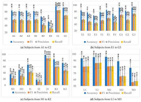
Figure 6.
The SSTMNet model performance on all subjects.
As far as the parameter complexity of the model is concerned, it involves 1,047,981 learnable parameters, which provide enough capacity for the model to learn intricate EEG patterns to discriminate various MI tasks.
5.2. Ablation Study on Hyperparameters of Blocks
Various hyperparameters are involved in the SSTMNet blocks, as shown in Table 4. Several experiments were performed to find out the best value of each hyperparameter. Details are given in the following subsections.
5.2.1. Attention Block
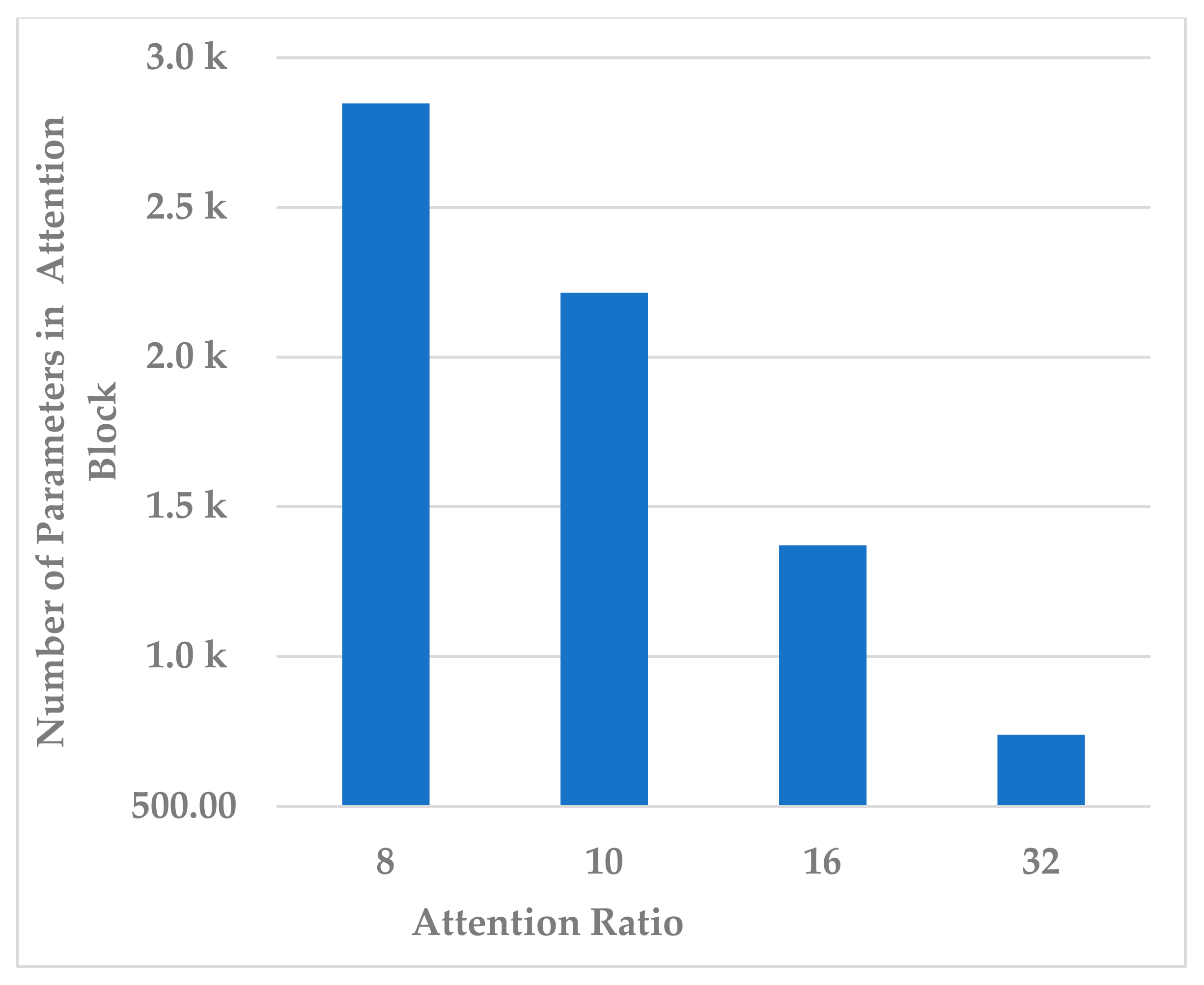
This block contains one hyperparameter, which is the compression ratio r. Different ratio values were examined, such as to analyze its effect on different performance measures and the model’s complexity. In terms of all measures, 10 and 32 almost gave the same results, but 32 resulted in less standard deviation in all measures, as shown in Figure 7. In addition, the complexity of the attention block decreased significantly when the ratio increased to 32, as can be seen in Figure 8. It can be concluded that the best ratio in the attention block was 32 in terms of model performance, stability, and block complexity.
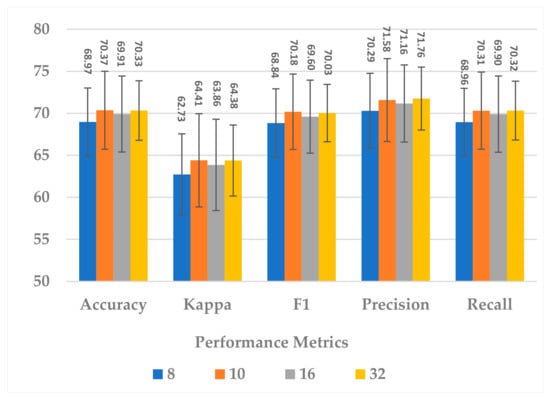
Figure 7.
The effect of attention block ratio on the SSTMNet model performance.

Figure 8.
The effect of attention block ratio on the attention block complexity.
5.2.2. Temporal Dependency Block
This block involves two hyperparameters, the number of neurons and number of layers . Two sets of experiments were conducted sequentially. First, different experiments were performed with to explore its impact on model performance and block complexity. The results are shown in Figure 9. The best results with slight differences were obtained when or , and the model seemed to be stable when , as shown in Figure 9. However, when , the block complexity significantly increased (about 277%), causing overfitting (see Figure 10). As a result, was preferred over due to a significant increase in the number of learnable parameters. The results show a direct relationship between all performance measures and the number of neurons.
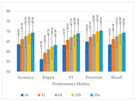
Figure 9.
The effect of number of neurons in GRU layers of temporal dependency block on the SSTMNet model performance.
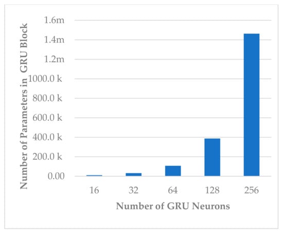
Figure 10.
The effect of number of neurons on temporal dependency block complexity.
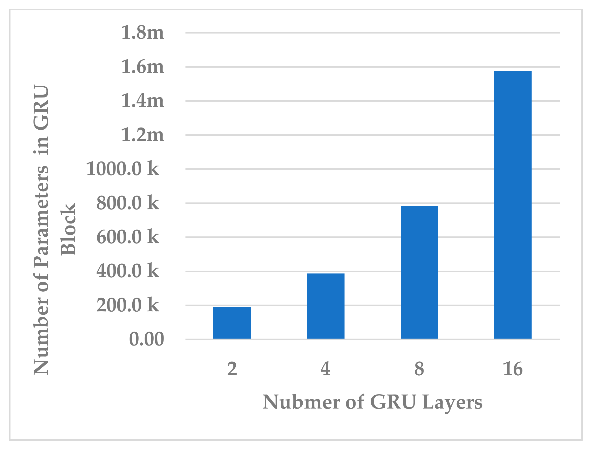
Afterwards, the effect of the number of layers was evaluated using L = 2, 4, 8, 16. The number of layers in the temporal dependency block reveals an inverse relationship in terms of all performance measures. The best performance was obtained when (see Figure 11). In this case, the learnable parameter complexity of the block was reduced by half (see Figure 12).
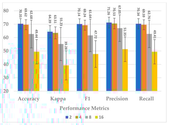
Figure 11.
The effect of number of layers in temporal dependency on the SSTMNet model performance.

Figure 12.
The effect of number of layers on temporal dependency block complexity.
5.2.3. Multiscale Block
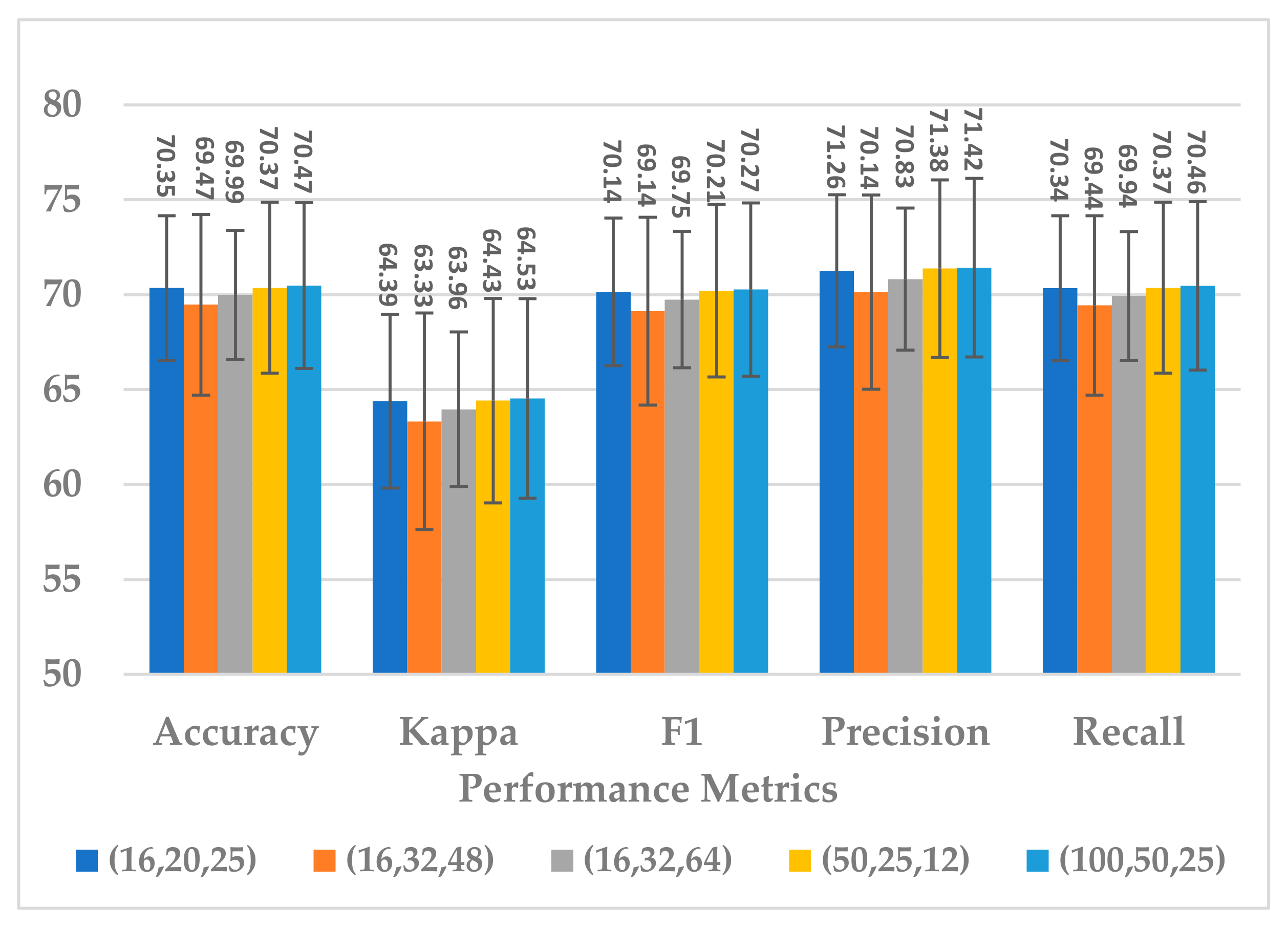
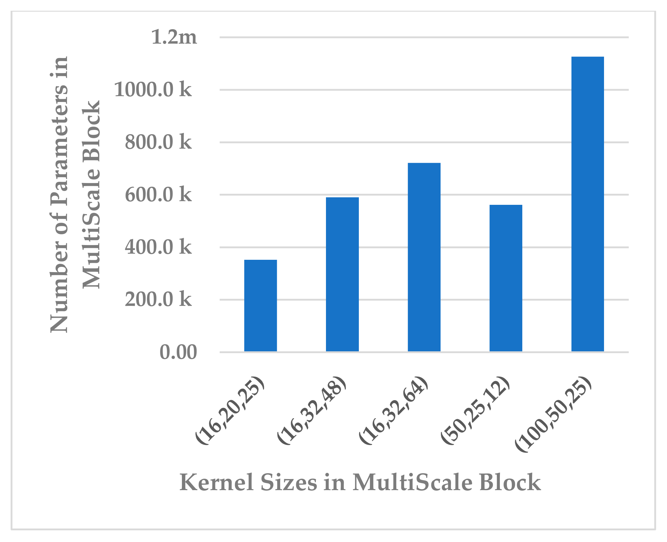
This block was employed to extract high-level features at different scales with a view to handle inter and intra-subject variabilities [36]. Different scales were analyzed that were selected to be divisible by two, the power of two, and the sample rate over the power of two, as shown in Table 5. The kernel sizes , and yielded almost the same results for all performance metrics, as shown in Figure 13. Out of the three combinations, revealed a lower standard deviation and the parameter complexity of the block, as indicated in Figure 14. It was inferred that the is the best choice.
Table 5.
Different kernel sizes in multiscale blocks.
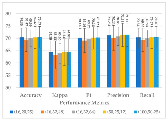
Figure 13.
The effect of kernel sizes in multiscale block on the SSTMNet model performance.

Figure 14.
The effect of kernel sizes in multiscale block on its parameter complexity.
5.2.4. Sequential Block
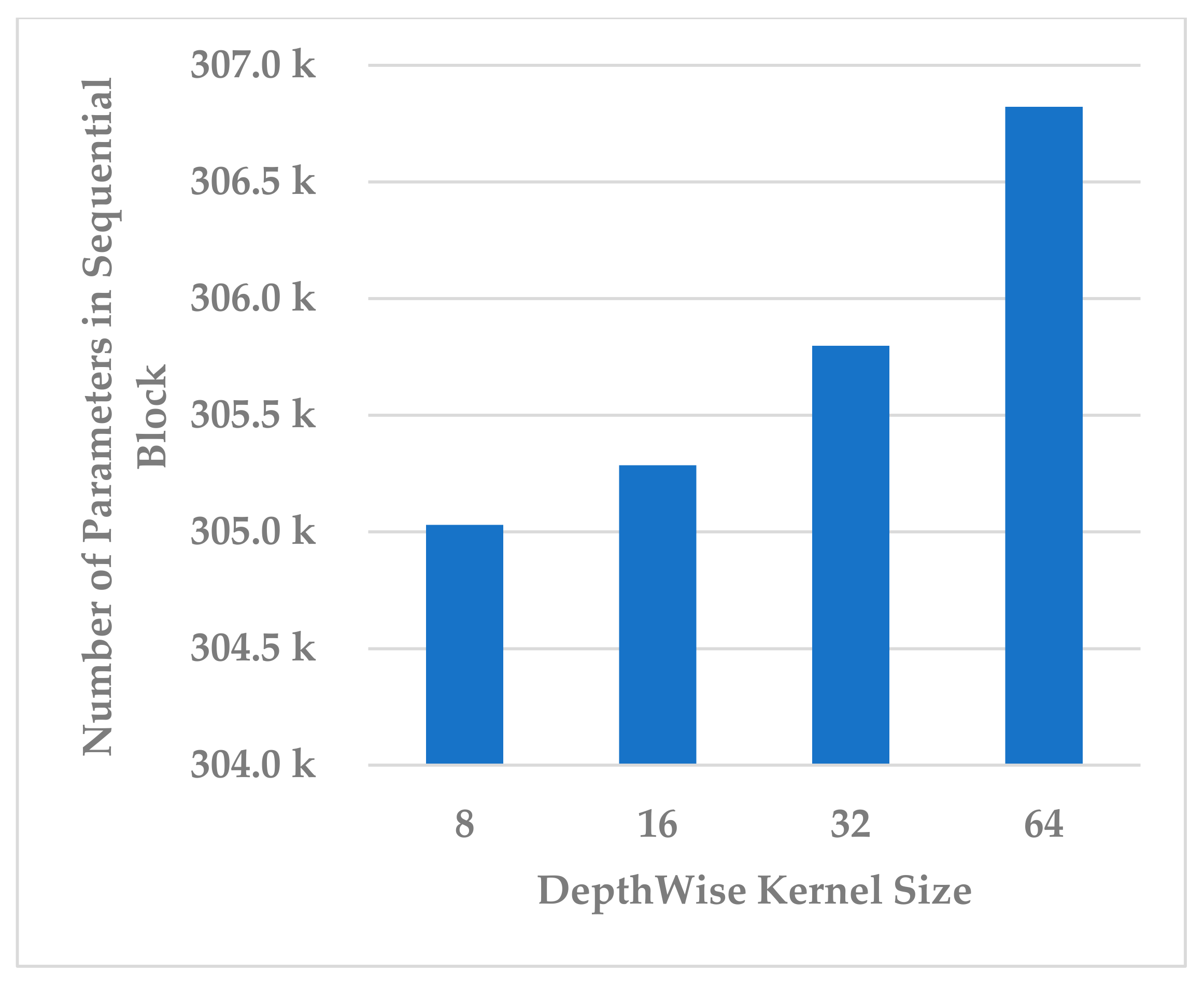
This block was utilized to detect high-level spectral–spatio-temporal features and reduce the model complexity by compressing the features along the channel and temporal dimensions. Two hyperparameters were independently analyzed, depth-wise kernel size and standard CNN kernel size.
Four depth-wise kernel sizes were tested, which included 8, 16, 32, and 64. The results shown in Figure 15 indicate that the depth-wise kernel size of 32 resulted in the best performance in terms of all metrics. A size less than 32 did not allow for learning of the discriminative features, and a size greater than 32 caused the learning of redundant features, which affected the model’s performance. Further, this choice of the size had the best compromise for the complexity of the sequential block, as is depicted in Figure 16.
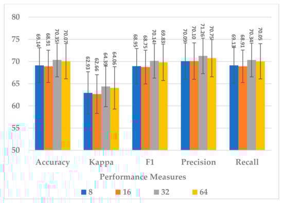
Figure 15.
The effect of the kernel size in the depth-wise Conv. layer of sequential block on the SSTMNet model performance.

Figure 16.
The effect of kernel size of depth-wise Conv. layer on sequential block complexity.
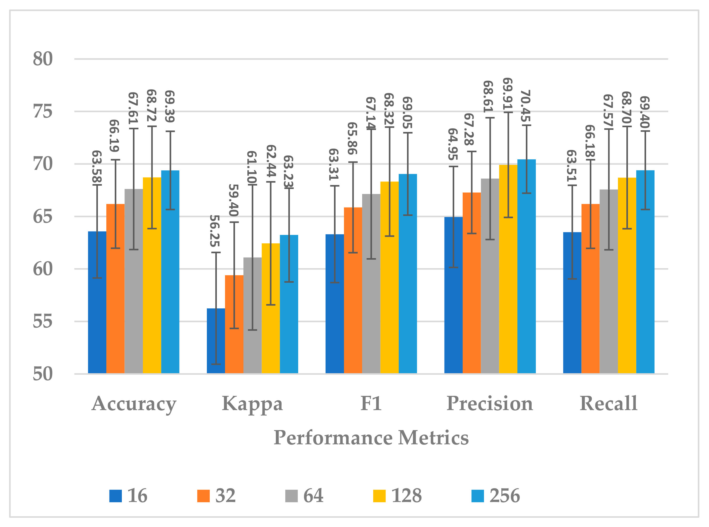
The kernel size of the standard CNN has a significant effect on the complexity of the block, as it is followed by the fully connected layer. It was endeavored to select a kernel size that best compromised between model performance, generalization, and block complexity. The following four choices were considered: 8, 16, 32, and 64. The results in Figure 17 show that, even in this case, the size of 32 was the best choice in terms of all metrics. However, the results for size 16 were close to those of 32 and more stable because the standard deviation in this was less. Further, the block complexity decreased by 71.99% compared to the kernel size of 32, as shown in Figure 18. In view of this significant decrease in the block complexity, the best choice was 16.
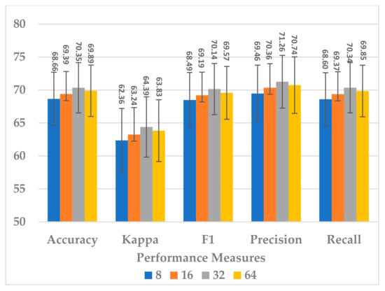
Figure 17.
The effect of the kernel size in the standard Conv. layer of sequential block on the SSTMNet model performance.
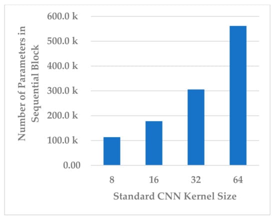
Figure 18.
The effect of kernel size of standard Conv. layer on sequential block complexity.
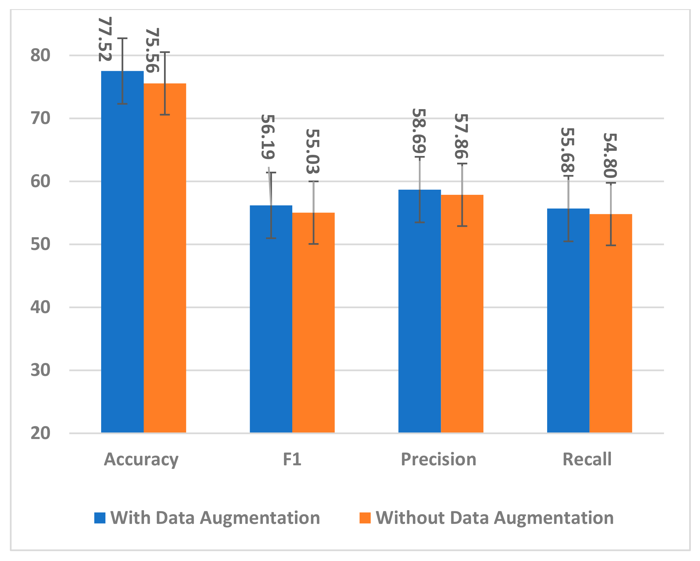
5.3. Impact of Data Augmentation
The proposed data augmentation method was used to handle the small dataset problem and effectively train the model by exposing it to many augmented trials. The number of training samples was quadrupled to overcome overfitting and improve the model generalization to unseen samples. To ensure the effectiveness of augmented trials in training the model, two experiments with and without data augmentation were conducted. The model, trained on only the original dataset, showed a decrease across all performance measures, as is evident from Figure 19.

Figure 19.
The impact of data augmentation on the SSTMNet model performance.
By observing individual subject accuracy with and without data augmentation, it is noticed that all subjects’ performance improved significantly with data augmentation, except for A3, which showed a small decrease. All trials created by interpolation and extrapolation contributed to the model’s effectiveness in training and producing good results for unseen samples.
5.4. Comparison to the State-of-the-Art Methods
To validate and ensure the effectiveness of SSTMNet, it was compared with the state-of-the-art methods on the same dataset, i.e., the HaLT paradigm. The focus was on the methods that used all six classes, all subjects, and sessions. SSTMNet was compared with the methods that followed the subject-dependent protocol evaluation, and the results reported were session-wise. The comparison is presented in Table 6.
Table 6.
Subject-wise and session-wise comparison of SSTMNet with the state-of-the-art methods.
George et al. [13] evaluated different data augmentation methods using DeepNet. George et al. [14] employed within- and cross-subject transfer learning, in addition to a subject-dependent protocol using BiGRU, DeepNet, and multi-branch Shallow network [18]. The SD protocol yielded (77.70 ± 11.06, 81.49 ± 11.3, and 78.32 ± 7.53) using the DL models mentioned above. The studies in [13,14] only revealed an average accuracy and no information about session-wise accuracy. George et al. [29] conducted a comparative study to compare the SOTA classifiers, DL models with trial-wise and cropping methods, and SOTA feature extraction methods with DL models as classifiers. In the references [13,29], the accuracy was reported as 83.01% and 81.92%, respectively. However, this accuracy was obtained after applying many preprocessing techniques such as bandpass filter, baseline correction, artifact correction, and data re-referencing. In addition, the studies in [13,14,29] conducted trial rejections without revealing the procedures for rejecting trials and the number of rejected trials.
Yan et al. [31] utilized a graph CNN with an attention mechanism and reshaped the raw signal into two graph representations, spatial–temporal and spatial–spectral representations, achieving an average accuracy of 81.61%. However, removing the attention block degraded the performance by 8.10%. Mwata-Velu et al. [30] proposed two preprocessing approaches to select the six and eight most discriminative channels using EEGNet for preprocessing and evaluation. Although the average accuracy reached 83.79%, the number and name of channels varied across subjects, which cannot be applied in real-world applications. Additionally, the model was trained for 1500 epochs and 10-folds, which is time-consuming. Both studies combined all sessions per subject to train, validate, and test DL models.
Due to the similar evaluation protocol, the accuracy achieved in this work is compared to those of [24,29]. It is worth mentioning that the trial rejection process was not employed to fairly evaluate the proposed model for classifying MI tasks. It achieved an accuracy of 77.52% ± 4.00 by computing the average of 10 folds and 83.76% by reporting the best fold that outperformed work in [29]. Furthermore, the majority of subjects performed better in this work compared to the results in [29] (see Table 6). Additionally, there was no significant difference between the maximum values of SSTMNet and those in [29], and the differences were not significant at the 5% significance level. The proposed model resulted in an average accuracy improvement of 19.13% in comparison to the method by Kaya et al. [24]. Furthermore, the mean performance of SSTMNet was significantly better than that of the method by Kaya et al. [24] at the 5% significance level (p-value = 7 × 10⁻¹¹). Finally, it should be pointed out that the subject-wise results of Kaya et al. [24] were obtained from the study in [29].
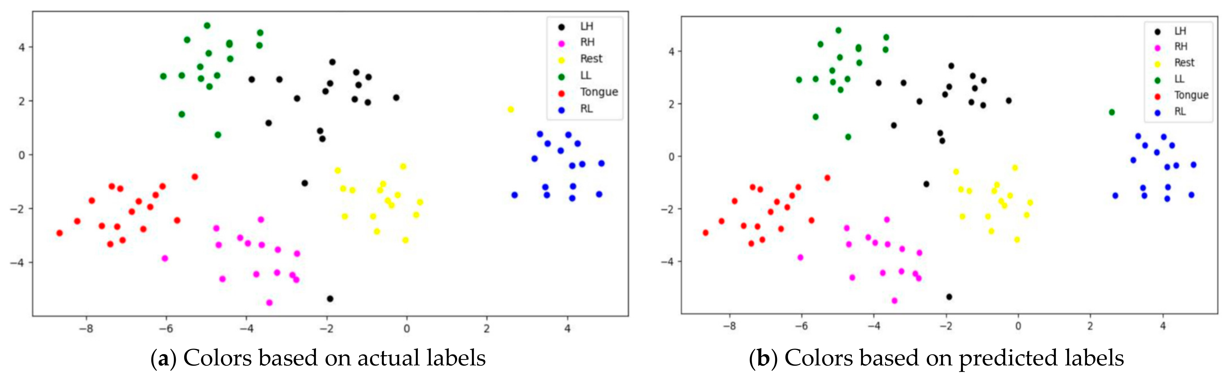
5.5. Feature Visualization Based on t-SNE
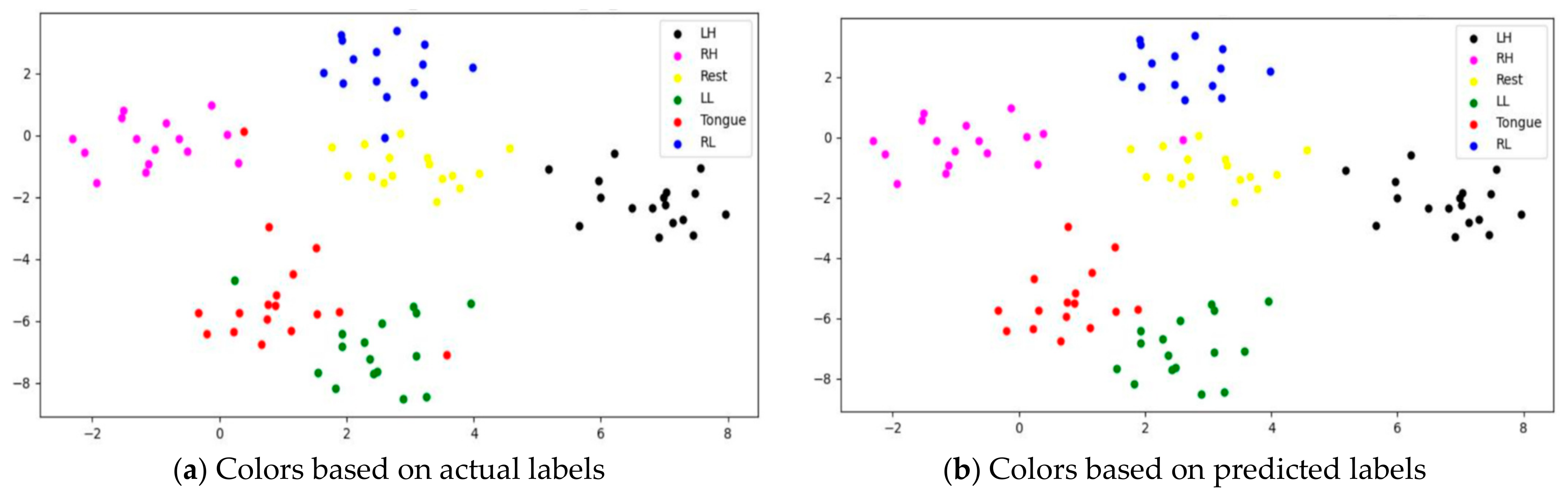
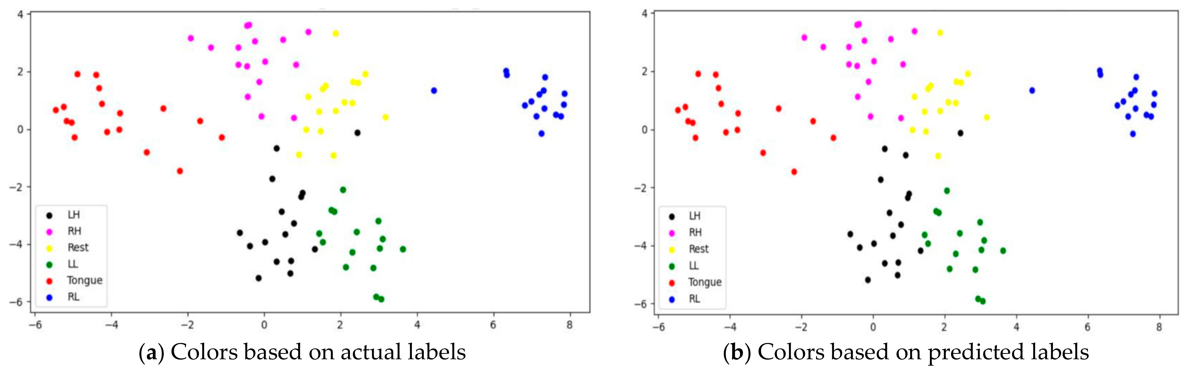
To assess whether SSTMNet learned discriminative features, three subjects, C1, G3, and L2, were selected, and their features learned by the model were plotted using t-SNE, as shown in Figure 20, Figure 21 and Figure 22. It is clear from these figures that the features of all trials were well-clustered and separated.
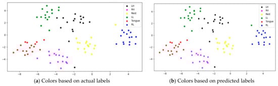
Figure 20.
The t-SNE plot representing extracted features of the subject C1.
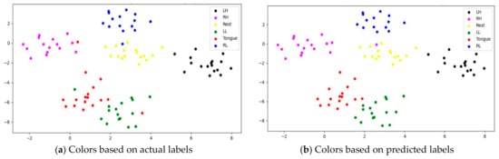
Figure 21.
The t-SNE plot representing extracted features of the subject G3.
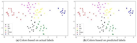
Figure 22.
The t-SNE plot representing extracted features of the subject the subject L2.
However, passive state features were classified as left leg and hand in subjects C1 and L2, respectively. Figure 21 depicts the misclassification of only two tongue cases and two different sides of leg movements in subject G3. The misclassification was due to the consistency of features extracted from tongue, right hand, and left leg movements in subject G3, and rest and left hand in subject L2. In addition, other misclassified cases could be caused by label noise and imagining different movements. Overall, the proposed model was able to extract discriminative features after processing signals through the attention, temporal dependency, multiscale, and sequential blocks.
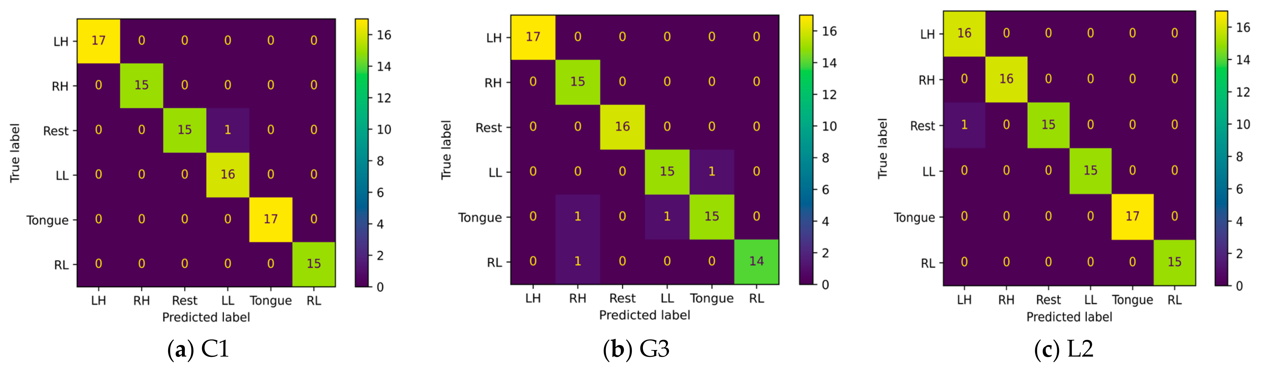
5.6. Confusion Matrix
A confusion matrix is an interpretation method that provides insight into a model’s decision making and helps to identify correctly classified and misclassified trials and their relationships. By investigating the confusion matrix and t-SNE plots at the same time, we can determine tasks that are difficult to discriminate due to either similarity in the features extracted by the model or label noise. Figure 23 shows the confusion matrices for six imagery tasks of three subjects, C1, G3, and L2. The presented confusion matrices show consistency with t-SNE feature plots. Only one rest case was misclassified in subjects C1 and L2 with left leg and hand movements, as presented in Figure 23a,c. Furthermore, two cases of tongue movements and one case of right hand and left leg movements were misclassified in subject G3.
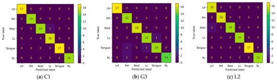
Figure 23.
Confusion matrices of three subjects: (a) C1, (b) G3, and (c) L1.
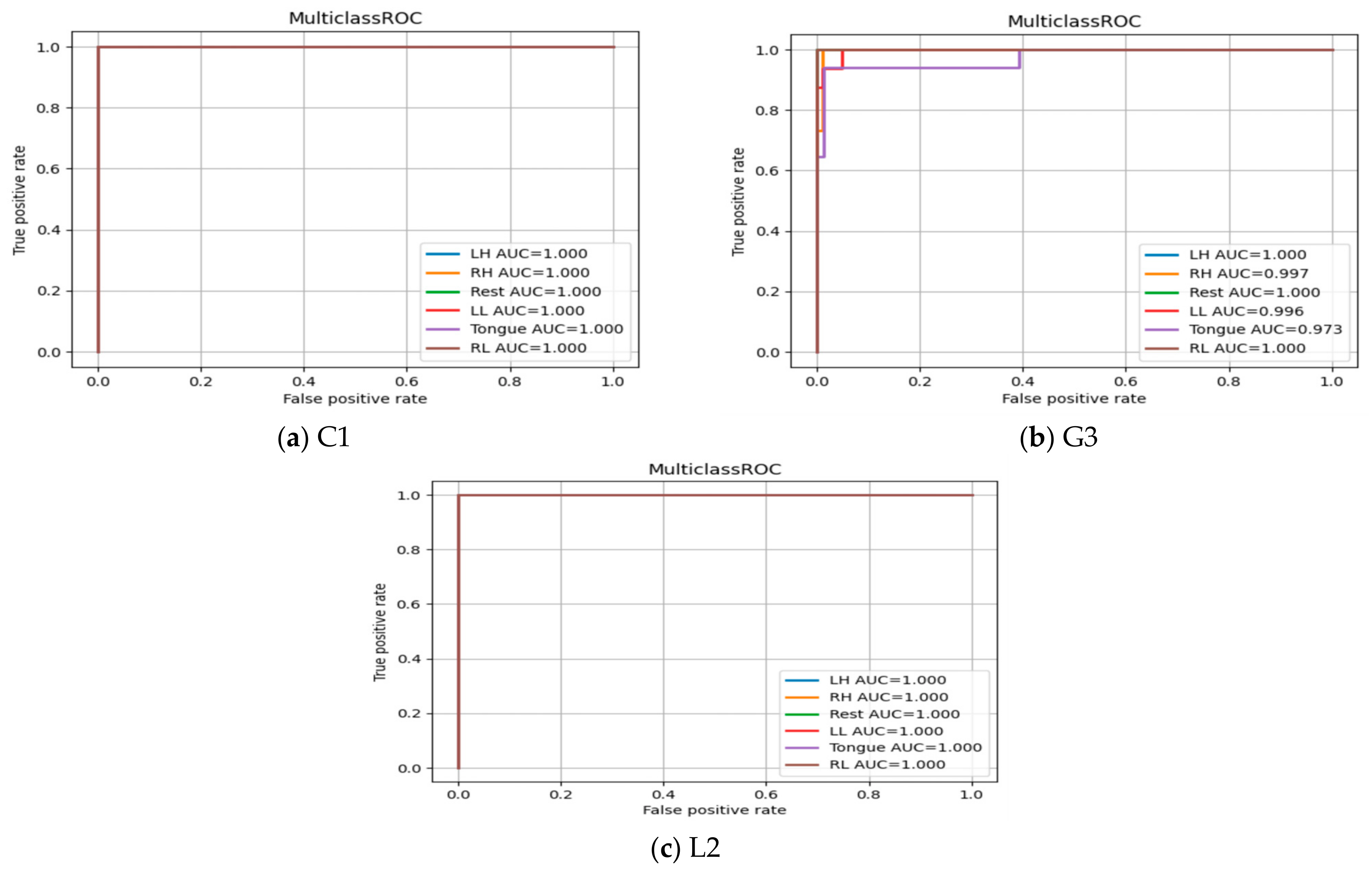
5.7. ROC Curve for Multiclass Classification
The Receiver Operating Characteristic (ROC) curves are presented in Figure 24 for subjects C1, G3, and L2. It shows the true positive rate (TPR) and false positive rate (FPR) for each MI task at different thresholds values to show the effectiveness of classifier in predicting MI tasks correctly. The area under the curve (AUC) in all three subjects and among six MI tasks produces a high value (above 0.90), which indicates the robustness of the SSTMNet in discriminating each MI task accurately.
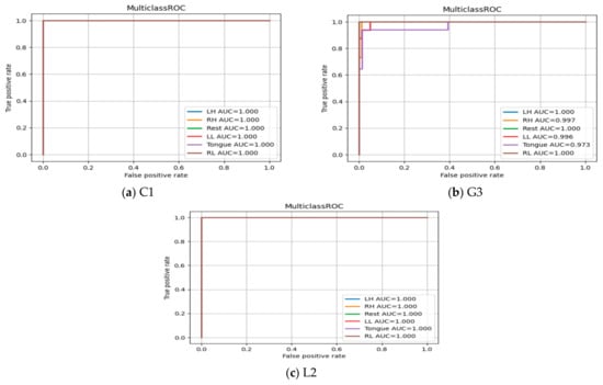
Figure 24.
ROC Curve of three subjects: (a) C1, (b) G3, and (c) L2.
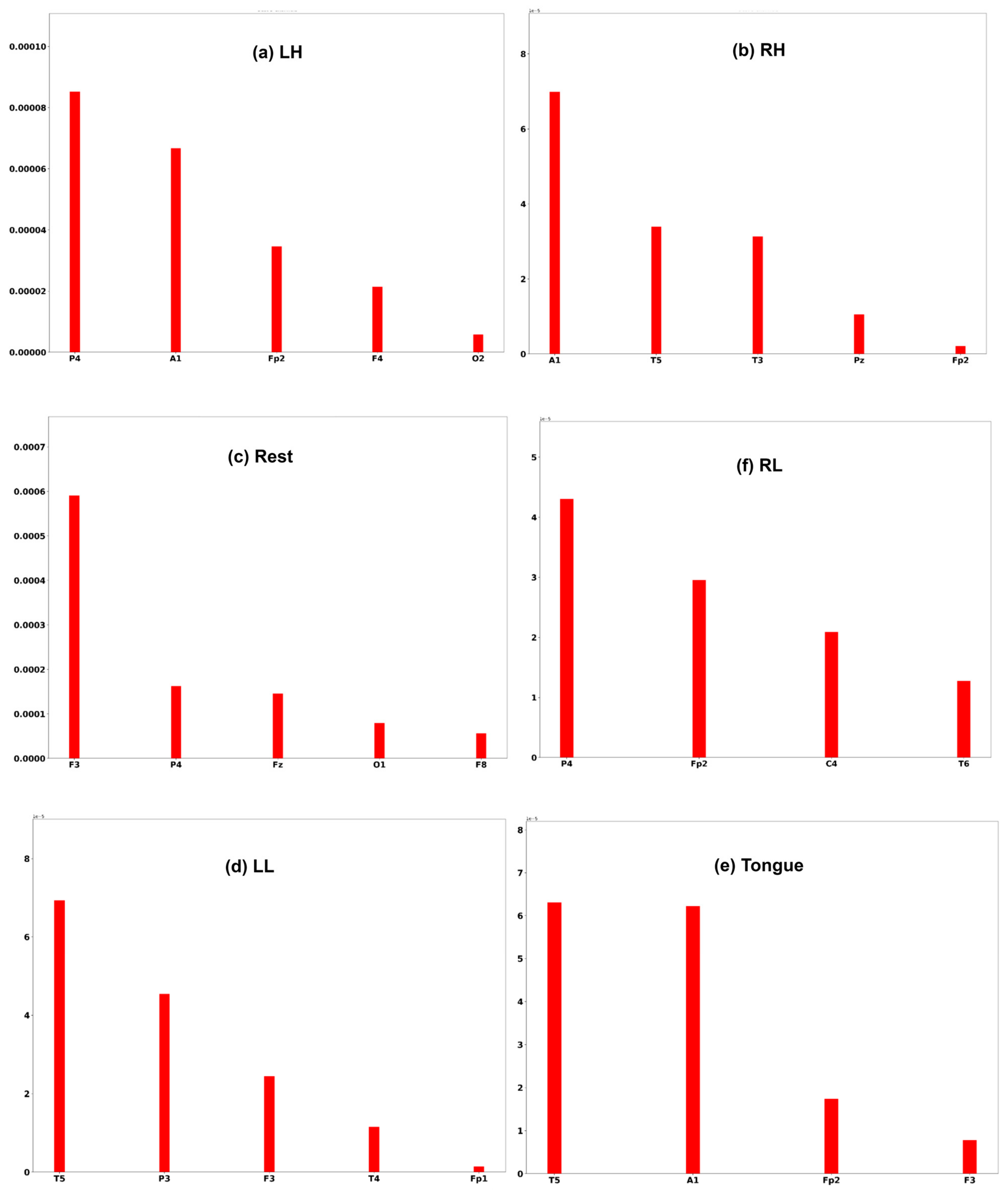
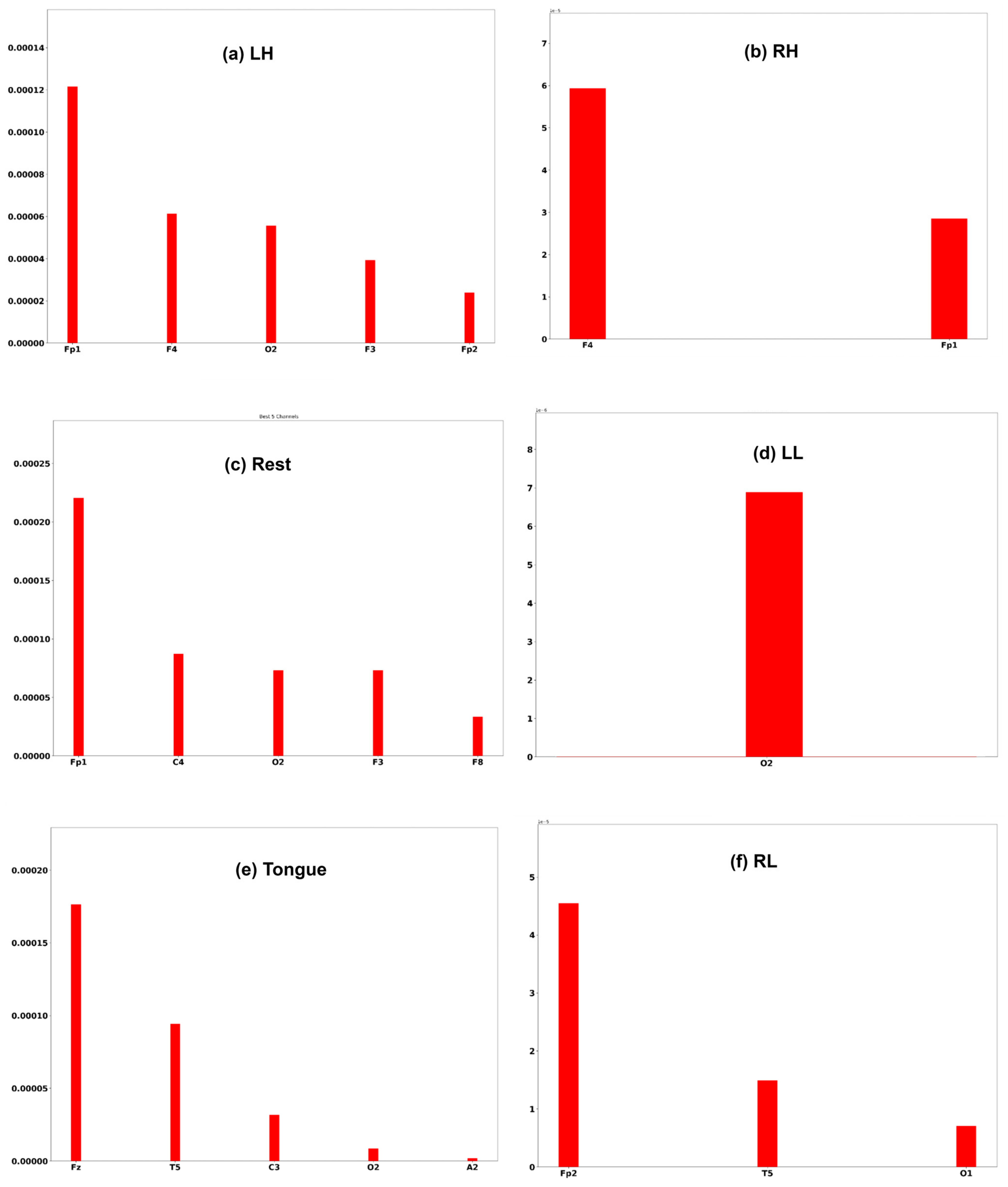
5.8. The Most Effective Channel in Each MI Tasks Based on SHAP Value
A commonly used interpretation techniques, namely Shapley Additive Explanation [47], has been employed to measure the effectiveness of channels of an EEG signal in model performance. In order to interpret the model prediction results and understand which channels help the model to reach the correct decision, the DeepLift SHAP technique [48] is used.
Three subjects, C1, G3, and L2, are chosen to interpret the model prediction. Each of the Figure 25, Figure 26 and Figure 27 displays the channels that have a positive impact on predicting the MI task. The positive average SHAP values of the channels with the nominated channels are depicted on the x-axis and the y-axis.
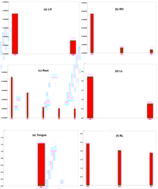
Figure 25.
SHAP values for the best channels in each class of subject C1.

Figure 26.
SHAP values for the best channels in each class of subject G3.

Figure 27.
SHAP values for the best channels in each class of subject L2.
It is obvious that the performance of the model is greatly influenced by the channels of the frontal and temporal lobes in all three subjects. Additionally, different MI tasks are affected by different groups of channels. The most common channels that obtained a positive SHAP value among the three subjects in different MI tasks are as follows:
6. Discussion
The SSTMNet model achieved an accuracy of 83.76%, 68.70%,70.61%, and 69% in F1 score, precision, and recall by computing the average of the best fold. Furthermore, almost 50% of subjects achieved an accuracy above 90%, and 10 subjects achieved above 80% for the remaining performance metrics. The SSTMNet model was also able to achieve a 100% and 99% accuracy in many subjects, such as C (session 1), J (session 1), L (session 2), and M (session 1). By comparing the average results obtained with the state-of-the-art models presented in Table 6, the SSTMNet model produced a higher accuracy in more than half of the subjects.
These reported results demonstrate the significance of performing spectral analysis and magnifying brain waves relevant to MI tasks. In addition, analyzing the long-term temporal dependencies among brain waves and inspecting multiscale and high-level features assist in adequately detecting motor imagery tasks. The proposed data augmentation was also able to expand the size of the dataset and effectively maintain label-preserving. This is reflected in the performance of the SSTMNet model, which overcomes overfitting and produces a higher accuracy compared to training the SSTMNet model without data augmentation.
The SSTMNet model achieved a good accuracy in terms of average and subject-wise results without using intensive preprocessing or trial rejection techniques, as presented in studies [13,14,29]. This indicates the robustness of the SSTMNet model to noise and artifacts. Most of the works that were presented utilized deep learning models such as EEGNet, DeepnNet, and shallowNet. However, in the SSTMNet model, the effectiveness of analyzing the frequency bands was explored by decomposing and reshaping signals in such a way that they could be meaningfully recalibrated using the attention mechanism. Afterward, the impact of integrating the temporal dependency block, sequential, and parallel CNN layers in detecting salient features related to the MI tasks was also studied. The t-SNE plots and confusion matrices presented in Section 5.5 and Section 5.6 showed the ability of the SSTMNet to target meaningful features. They also help, to some extent, in identifying the reasons for misclassified cases, such as the similarity between extracted MI features or label noise.
Although the SSTMNet achieved a high accuracy in many subjects, it still performed poorly in some cases, such as B (sessions 2, 3), E (session 3), F (session 3), H and I (all sessions), and k (session 2). These cases require a deep analysis of their EEG signals to determine the reasons behind their poor results and to ensure whether there is a label noise in the poor cases. Furthermore, The SSTMNet model was created by using a deep block architectural design that resulted in a complex model, which requires various techniques to handle its complexity. In the future work, channels reduction and Low-Rank Adaption (LoRA) methods will be used to reduce the model’s complexity
To sum up, the SSTMNet model and data augmentation methods achieved comparable average accuracy results and a higher accuracy in almost half of the subjects compared with the state-of-the-art methods with only local channel standardization and spectral decomposition.
7. Conclusions and Outlook
This paper aimed to use deep learning techniques to detect over four MI tasks present in EEG signals during imaging movements. The proposed SSTMNet model performed a spectral analysis and extracted high-level spectral–spatio-temporal features. Furthermore, the SSTMNet was trained on augmented trials generated from the existing EEG trials after being transformed into the frequency domain. This was accomplished by designing a block architectural model that involved attention, temporal dependency, and parallel and sequential CNN blocks. The proposed model had a comparable accuracy to the SOAT work using 10-fold CV and subject-specific protocol. It reached an average accuracy of 77.52% for 10 folds, and a max fold of 83.76%, without the need for advanced preprocessing methods such as trial rejections. These results were yielded by analyzing the EEG signals spectrally, maintaining long-term temporal dependencies between frequency bands, and finally detecting high-level features. It demonstrated the importance of EEG signal spectral analysis and working out short-term and long-term dependencies between them. It also indicated the effectiveness of augmented trials in training the model and ensuring that the frequency interpolation between trials produced effective trials rather than noise. While the study achieved good results in classifying more than four MI tasks, it focused on a subject-specific protocol and included all EEG channels. In future work, the focus will be on employing channel reduction methods and Low-Rank Adaptation (LoRA) to reduce the model complexity and enhance the overall accuracy.
Author Contributions
Conceptualization, A.A. and M.H.; methodology, A.A. and M.H.; software, A.A.; validation, A.A.; formal analysis, A.A. and M.H.; data curation, A.A. and M.H.; writing—original draft preparation, A.A.; writing—review and editing, A.A. and M.H.; visualization, A.A.; supervision, M.H. and H.A.; project administration, M.H.; funding acquisition, M.H. All authors have read and agreed to the published version of the manuscript.
Funding
The research was supported under Researchers Supporting Project number (RSP2025R109) King Saud University, Riyadh, Saudi Arabia.
Data Availability Statement
Public dataset was utilized in our work. Large EEG MI dataset for EEG Brain Computer Interface available at https://springernature.figshare.com/collections/A_large_electroencephalographic_motor_imagery_dataset_for_electroencephalographic_brain_computer_interfaces/3917698 (accessed on 20 January 2022).
Conflicts of Interest
The authors declare no competing interests.
References
- Mary, P.; Servais, L.; Vialle, R. Neuromuscular Diseases: Diagnosis and Management. Orthop. Traumatol. Surg. Res. 2018, 104, S89–S95. [Google Scholar] [CrossRef] [PubMed]
- Institute for Disability Research, Policy, and Practice WebAIM: Motor Disabilities-Types of Motor Disabilities. Available online: https://webaim.org/articles/motor/motordisabilities (accessed on 13 November 2024).
- Värbu, K.; Muhammad, N.; Muhammad, Y. Past, Present, and Future of EEG-Based BCI Applications. Sensors 2022, 22, 3331. [Google Scholar] [CrossRef] [PubMed]
- Aggarwal, S.; Chugh, N. Signal Processing Techniques for Motor Imagery Brain Computer Interface: A Review. Array 2019, 1–2, 100003. [Google Scholar] [CrossRef]
- Oikonomou, V.P.; Georgiadis, K.; Liaros, G.; Nikolopoulos, S.; Kompatsiaris, I. A Comparison Study on EEG Signal Processing Techniques Using Motor Imagery EEG Data. In Proceedings of the 2017 IEEE 30th International Symposium on Computer-Based Medical Systems (CBMS), Thessaloniki, Greece, 22–24 June 2017; pp. 781–786. [Google Scholar]
- Orban, M.; Elsamanty, M.; Guo, K.; Zhang, S.; Yang, H. A Review of Brain Activity and EEG-Based Brain–Computer Interfaces for Rehabilitation Application. Bioengineering 2022, 9, 768. [Google Scholar] [CrossRef]
- Nicolas-Alonso, L.F.; Gomez-Gil, J. Brain Computer Interfaces, a Review. Sensors 2012, 12, 1211–1279. [Google Scholar] [CrossRef]
- Ang, K.K.; Guan, C. EEG-Based Strategies to Detect Motor Imagery for Control and Rehabilitation. IEEE Trans. Neural Syst. Rehabil. Eng. 2017, 25, 392–401. [Google Scholar] [CrossRef]
- Ang, K.K.; Guan, C.; Chua, K.S.G.; Ang, B.T.; Kuah, C.; Wang, C.; Phua, K.S.; Chin, Z.Y.; Zhang, H. Clinical Study of Neurorehabilitation in Stroke Using EEG-Based Motor Imagery Brain-Computer Interface with Robotic Feedback. In Proceedings of the 2010 Annual International Conference of the IEEE Engineering in Medicine and Biology, Buenos Aires, Argentina, 31 August–4 September 2010; Volume 2010, pp. 5549–5552. Available online: https://doi.org/10.1109/IEMBS.2010.5626782 (accessed on 7 September 2023). [CrossRef]
- Yang, K.; Li, R.; Xu, J.; Zhu, L.; Kong, W.; Zhang, J. DSFE: Decoding EEG-Based Finger Motor Imagery Using Feature-Dependent Frequency, Feature Fusion and Ensemble Learning. IEEE J. Biomed. Health Inform. 2024, 28, 4625–4635. [Google Scholar] [CrossRef]
- Degirmenci, M.; Yuce, Y.K.; Perc, M.; Isler, Y. EEG-Based Finger Movement Classification with Intrinsic Time-Scale Decomposition. Front. Hum. Neurosci. 2024, 18, 1362135. [Google Scholar] [CrossRef]
- Lian, S.; Li, Z. An End-to-End Multi-Task Motor Imagery EEG Classification Neural Network Based on Dynamic Fusion of Spectral-Temporal Features. Comput. Biol. Med. 2024, 178, 108727. [Google Scholar] [CrossRef]
- George, O.; Smith, R.; Madiraju, P.; Yahyasoltani, N.; Ahamed, S.I. Data Augmentation Strategies for EEG-Based Motor Imagery Decoding. Heliyon 2022, 8, e10240. [Google Scholar] [CrossRef]
- George, O.; Dabas, S.; Sikder, A.; Smith, R.; Madiraju, P.; Yahyasoltani, N.; Ahamed, S.I. Enhancing Motor Imagery Decoding via Transfer Learning. Smart Health 2022, 26, 100339. [Google Scholar] [CrossRef]
- Mishuhina, V.; Jiang, X. Complex Common Spatial Patterns on Time-Frequency Decomposed EEG for Brain-Computer Interface. Pattern Recognit. 2021, 115, 107918. [Google Scholar] [CrossRef]
- Miao, Y.; Jin, J.; Daly, I.; Zuo, C.; Wang, X.; Cichocki, A.; Jung, T.-P. Learning Common Time-Frequency-Spatial Patterns for Motor Imagery Classification. IEEE Trans. Neural Syst. Rehabil. Eng. 2021, 29, 699–707. [Google Scholar] [CrossRef]
- Lawhern, V.J.; Solon, A.J.; Waytowich, N.R.; Gordon, S.M.; Hung, C.P.; Lance, B.J. EEGNet: A Compact Convolutional Network for EEG-Based Brain-Computer Interfaces. J. Neural Eng. 2018, 15, 056013. [Google Scholar] [CrossRef] [PubMed]
- Schirrmeister, R.T.; Springenberg, J.T.; Fiederer, L.D.J.; Glasstetter, M.; Eggensperger, K.; Tangermann, M.; Hutter, F.; Burgard, W.; Ball, T. Deep Learning with Convolutional Neural Networks for EEG Decoding and Visualization. Hum. Brain Mapp. 2017, 38, 5391–5420. [Google Scholar] [CrossRef] [PubMed]
- Padfield, N.; Zabalza, J.; Zhao, H.; Masero, V.; Ren, J. EEG-Based Brain-Computer Interfaces Using Motor-Imagery: Techniques and Challenges. Sensors 2019, 19, 1423. [Google Scholar] [CrossRef]
- Decety, J.; Sjöholm, H.; Ryding, E.; Stenberg, G.; Ingvar, D.H. The Cerebellum Participates in Mental Activity: Tomographic Measurements of Regional Cerebral Blood Flow. Brain Res. 1990, 535, 313–317. [Google Scholar] [CrossRef]
- Yilmaz, C.M.; Yilmaz, B.H. Advancements in Image Feature-Based Classification of Motor Imagery EEG Data: A Comprehensive Review. Trait. Signal 2023, 40, 1857–1868. [Google Scholar] [CrossRef]
- Altaheri, H.; Muhammad, G.; Alsulaiman, M.; Amin, S.U.; Altuwaijri, G.A.; Abdul, W.; Bencherif, M.A.; Faisal, M. Deep Learning Techniques for Classification of Electroencephalogram (EEG) Motor Imagery (MI) Signals: A Review. Neural Comput. Applic 2023, 35, 14681–14722. [Google Scholar] [CrossRef]
- Gwon, D.; Won, K.; Song, M.; Nam, C.S.; Jun, S.C.; Ahn, M. Review of Public Motor Imagery and Execution Datasets in Brain-Computer Interfaces. Front. Hum. Neurosci. 2023, 17, 1134869. [Google Scholar] [CrossRef]
- Kaya, M.; Binli, M.K.; Ozbay, E.; Yanar, H.; Mishchenko, Y. A Large Electroencephalographic Motor Imagery Dataset for Electroencephalographic Brain Computer Interfaces. Sci. Data 2018, 5, 180211. [Google Scholar] [CrossRef] [PubMed]
- Ofner, P.; Schwarz, A.; Pereira, J.; Müller-Putz, G.R. Upper Limb Movements Can Be Decoded from the Time-Domain of Low-Frequency EEG. PLoS ONE 2017, 12, e0182578. [Google Scholar] [CrossRef]
- Yi, W.; Qiu, S.; Wang, K.; Qi, H.; Zhang, L.; Zhou, P.; He, F.; Ming, D. Evaluation of EEG Oscillatory Patterns and Cognitive Process during Simple and Compound Limb Motor Imagery. PLoS ONE 2014, 9, e114853. [Google Scholar] [CrossRef] [PubMed]
- Jeong, J.-H.; Cho, J.-H.; Shim, K.-H.; Kwon, B.-H.; Lee, B.-H.; Lee, D.-Y.; Lee, D.-H.; Lee, S.-W. Multimodal Signal Dataset for 11 Intuitive Movement Tasks from Single Upper Extremity during Multiple Recording Sessions. GigaScience 2020, 9, giaa098. [Google Scholar] [CrossRef] [PubMed]
- Wirawan, I.M.A.; Maneetham, D.; Darmawiguna, I.G.M.; Niyomphol, A.; Sawetmethikul, P.; Crisnapati, P.N.; Thwe, Y.; Agustini, N.N.M. Acquisition and Processing of Motor Imagery and Motor Execution Dataset (MIMED) for Six Movement Activities. Data Brief 2024, 56, 110833. [Google Scholar] [CrossRef]
- George, O.; Dabas, S.; Sikder, A.; Smith, R.O.; Madiraju, P.; Yahyasoltani, N.; Ahamed, S.I. State-of-the-Art versus Deep Learning: A Comparative Study of Motor Imagery Decoding Techniques. IEEE Access 2022, 10, 45605–45619. [Google Scholar] [CrossRef]
- Mwata-Velu, T.; Niyonsaba-Sebigunda, E.; Avina-Cervantes, J.G.; Ruiz-Pinales, J.; Velu-A-Gulenga, N.; Alonso-Ramírez, A.A. Motor Imagery Multi-Tasks Classification for BCIs Using the NVIDIA Jetson TX2 Board and the EEGNet Network. Sensors 2023, 23, 4164. [Google Scholar] [CrossRef]
- Yan, Z.; Yang, X.; Jin, Y. Considerate Motion Imagination Classification Method Using Deep Learning. PLoS ONE 2022, 17, e0276526. [Google Scholar] [CrossRef]
- Lee, G.R.; Gommers, R.; Waselewski, F.; Wohlfahrt, K.; O’Leary, A. PyWavelets: A Python Package for Wavelet Analysis. J. Open Source Softw. 2019, 4, 1237. [Google Scholar] [CrossRef]
- Pattnaik, S.; Dash, M.; Sabut, S.K. DWT-Based Feature Extraction and Classification for Motor Imaginary EEG Signals. In Proceedings of the 2016 International Conference on Systems in Medicine and Biology (ICSMB), Kharagpur, India, 4–7 January 2016; IEEE: Kharagpur, India, 2016; pp. 186–201. [Google Scholar]
- Hamedi, M.; Salleh, S.-H.; Noor, A.M. Electroencephalographic Motor Imagery Brain Connectivity Analysis for BCI: A Review. Neural Comput. 2016, 28, 999–1041. [Google Scholar] [CrossRef]
- Naeem, M.; Brunner, C.; Leeb, R.; Graimann, B.; Pfurtscheller, G. Seperability of Four-Class Motor Imagery Data Using Independent Components Analysis. J. Neural Eng. 2006, 3, 208–216. [Google Scholar] [CrossRef] [PubMed]
- Jia, Z.; Lin, Y.; Wang, J.; Yang, K.; Liu, T.; Zhang, X. MMCNN: A Multi-Branch Multi-Scale Convolutional Neural Network for Motor Imagery Classification. In Proceedings of the Machine Learning and Knowledge Discovery in Databases, Ghent, Belgium, 14–18 September 2020; Hutter, F., Kersting, K., Lijffijt, J., Valera, I., Eds.; Springer International Publishing: Cham, Switzerland, 2021; pp. 736–751. [Google Scholar]
- Hu, J.; Shen, L.; Sun, G. Squeeze-and-Excitation Networks. In Proceedings of the IEEE Conference on Computer Vision and Pattern Recognition (CVPR), Salt Lake City, UT, USA, 18–22 June 2018; pp. 7132–7141. [Google Scholar]
- Gao, Y.; Glowacka, D. Deep Gate Recurrent Neural Network. In Proceedings of the 8th Asian Conference on Machine Learning, Hamilton, New Zealand, 16–18 November 2016. [Google Scholar]
- Bai, S.; Kolter, J.Z.; Koltun, V. An Empirical Evaluation of Generic Convolutional and Recurrent Networks for Sequence Modeling. arXiv 2018, arXiv:1803.01271. [Google Scholar]
- Cho, K.; van Merrienboer, B.; Gulcehre, C.; Bahdanau, D.; Bougares, F.; Schwenk, H.; Bengio, Y. Learning Phrase Representations Using RNN Encoder-Decoder for Statistical Machine Translation. 2014.
- Szegedy, C.; Liu, W.; Jia, Y.; Sermanet, P.; Reed, S.; Anguelov, D.; Erhan, D.; Vanhoucke, V.; Rabinovich, A. Going Deeper With Convolutions. In Proceedings of the 2015 IEEE Conference on Computer Vision and Pattern Recognition (CVPR); pp. 1–9.
- Akiba, T.; Sano, S.; Yanase, T.; Ohta, T.; Koyama, M. Optuna: A Next-Generation Hyperparameter Optimization Framework. In Proceedings of the 25th ACM SIGKDD International Conference on Knowledge Discovery & Data Mining, Anchorage, AK, USA, 4–8 August 2019. [Google Scholar]
- Chollet, F. Xception: Deep Learning with Depthwise Separable Convolutions. In Proceedings of the 30th IEEE Conference on Computer Vision and Pattern Recognition (CVPR), Honolulu, HI, USA, 21–26 July 2017. [Google Scholar]
- Heckbert, P.S. Fourier Transforms and the Fast Fourier Transform (FFT) Algorithm. Comput. Graph. 1998, 2, 15–463. [Google Scholar]
- Uyulan, C. Development of LSTM&CNN Based Hybrid Deep Learning Model to Classify Motor Imagery Tasks. bioRxiv 2020. [Google Scholar] [CrossRef]
- Hossin, M.; Sulaiman, M.N. A Review on Evaluation Metrics for Data Classification Evaluations. Int. J. Data Min. Knowl. Manag. Process 2015, 5, 1. [Google Scholar]
- Lundberg, S.M.; Lee, S.-I. A Unified Approach to Interpreting Model Predictions. In Proceedings of the 31st Conference on Neural Information Processing System, Long Beach, CA, USA, 4–9 December 2017. [Google Scholar]
- Kokhlikyan, N.; Miglani, V.; Martin, M.; Wang, E.; Alsallakh, B.; Reynolds, J.; Melnikov, A.; Kliushkina, N.; Araya, C.; Yan, S.; et al. Captum: A Unified and Generic Model Interpretability Library for PyTorch. Available online: https://captum.ai/ (accessed on 27 January 2025).


Disclaimer/Publisher’s Note: The statements, opinions and data contained in all publications are solely those of the individual author(s) and contributor(s) and not of MDPI and/or the editor(s). MDPI and/or the editor(s) disclaim responsibility for any injury to people or property resulting from any ideas, methods, instructions or products referred to in the content. |
© 2025 by the authors. Licensee MDPI, Basel, Switzerland. This article is an open access article distributed under the terms and conditions of the Creative Commons Attribution (CC BY) license (https://creativecommons.org/licenses/by/4.0/).