Article

Numerical Analysis of Time-Fractional Cancer Models with Different Types of Net Killing Rate

by
Hami Gündoǧdu
1,† and
Hardik Joshi
2,*,†
1
Department of Mathematics, Faculty of Science, Sakarya University, Serdivan 54050, Turkey
2
Department of Mathematics, LJ Institute of Engineering and Technology, LJ University, Ahmedabad 382210, Gujarat, India
*
Author to whom correspondence should be addressed.
These authors contributed equally to this work.
Mathematics 2025, 13(3), 536; https://doi.org/10.3390/math13030536
Submission received: 14 January 2025 / Revised: 31 January 2025 / Accepted: 3 February 2025 / Published: 6 February 2025

Abstract

:
This study introduces a novel approach to modeling cancer tumor dynamics within a fractional framework, emphasizing the critical role of the net killing rate in determining tumor growth or decay. We explore a generalized cancer model where the net killing rate is considered across three domains: time-dependent, position-dependent, and concentration-dependent. The primary objective is to derive an analytical solution for time-fractional cancer models using the Residual Power Series Method (RPSM), a technique not previously applied in this conformable context. Traditional methods for solving fractional-order differential models face challenges such as perturbations, complex simplifications, discretization issues, and restrictive assumptions. In contrast, the RPSM overcomes these limitations by offering a robust solution that reduces both complexity and computational effort. The method provides exact analytical solutions through a convergence series and reliable numerical approximations when needed, making it a versatile tool for simulating fractional-order cancer models. Graphical representations of the approximate solutions illustrate the method’s effectiveness and applicability. The findings highlight the RPSM’s potential to advance cancer treatment strategies by providing a more precise understanding of tumor dynamics in a fractional context. This work contributes to both theoretical and practical advancements in cancer research and lays the groundwork for more accurate and efficient modeling of cancer dynamics, ultimately aiding in the development of optimal treatment strategies.

1. Introduction

The complicated structure of cancer restricts treatment options, making it one of the most fatal diseases worldwide since it was first identified. Cancer encompasses a range of diseases marked by unchecked cell growth, resulting in the development of harmful tumors. Human cancer cells have antigens that the adaptive immune system can identify, providing a possible route to trigger an anticancer immune response. However, the complex and ever-changing interactions between tumor cells and their environment make developing effective treatments or cures a complex and demanding challenge. The initial step in cancer tumor formation involves alterations in specific genes, including tumor suppressor genes and proto-oncogenes. Cells with these genetic mutations gain a growth advantage over healthy cells, leading to increased genetic instability, making the cells more malignant and causing them to invade surrounding tissues. The complexities of tumor spread have driven many researchers to model and analyze this disease, especially using the Lie symmetry method. It also has drawn the interest of medical and biological scientists and applied mathematicians. Various approaches have been developed to study tumor growth and response to treatment. Mathematical models for cancer treatment have gained increasing significance over the years due to their ability to outline key immune system components involved in cancer therapy analytically. The earliest mathematical model for cancer treatment was proposed by Gompertz in 1825, focusing on tumor growth by accounting for both cell proliferation and cell death. Since then, research has frequently centered on how various components influence the tumor microenvironment. This microenvironment includes immune cells, signaling molecules, the extracellular matrix, fibroblasts, growth factors, and other connective tissue cells. Readers can check the papers [1,2,3,4,5,6,7,8,9,10] for further details.
Burgess et al. [11] proposed a diffusion-based model in which a spherical tumor, characterized by a proliferation rate p and a therapy-dependent killing rate k, is described by a governing equation:
C t ( r , t ) = D 1 r 2 r 2 C r ( r , t ) r + p C ( r , t ) k C ( r , t ) .
In this model, C ( r , t ) represents the concentration of tumor cells at time t and position r, while D denotes the diffusivity coefficient.
Moyo and Leach [12] proposed the following model of Equation (1) with a variable killing rate:
C x x ( x , t ) K ( x , t ) C ( x , t ) C t ( x , t ) = 0
by using the Lie symmetry method. K ( x , t ) denotes the net rate at which tumor cells are removed. It is worth noting that the therapy-dependent killing rate K can vary with both position and time rather than being constant or dependent on only time. Additionally, the examination of the model (2), in which the killing rate K ( u ) of cancer cells varies with cell concentration, led to a nonlinear version of the model.
Diseases such as malaria, dengue fever, infection, influenza, Ebola virus, and cancer have traditionally been modeled using ordinary differential equations of integer [13,14,15,16,17]. Recently, there has been a growing focus on fractional-order differential equations. Mathematical models employing fractional differential equations are essential for understanding tumor spread and interactions. The fractional tumor model provides insights into the dynamics of tumor and effector cells, offering a more nuanced and detailed analysis of cell behavior and the killing rate of cancer cells. Fractional modeling of cancer tumor differential equations has become a prominent topic in the recent literature. Studying cancer tumor models in their fractional form, as opposed to the classical integer form, offers several advantages. It allows for a more nuanced characterization of tumors at both spatial and temporal levels, leading to more accurate simulations of tumor growth dynamics. Additionally, it provides more precise insights into how various cell subpopulations respond to cancer therapy. Furthermore, these models can be employed by researchers and medical professionals to explore and develop treatment strategies for tumors. Farman et al. [18] analyzed a time-fractional tumor model in the context of vaccination. The cancer-immune system interplay using distinct fractional derivatives is investigated by Ucar and Ozdemir [19,20]. Barbosa et al. [21] attempted to find innovative ways for cancer tumor modeling to enhance the effectiveness of anticancer drugs. A tumor–immune system model related to lung cancer has been developed by Özköse et al. [22,23]. Kalal and Jha addressed cancer modeling by hidden Markov and machine learning techniques [24,25]. Mustapha et al. have examined the impact of viral load detectability on HIV/AIDS transmission with public awareness [26]. Raeisi et al. have examined the immune patterns and their effect on cancer cells by a deep learning algorithm [27]. Keshavarz et al. [28] addressed cancer tumor modeling in a fractional fuzzy environment using fuzzy integral transforms; check [29,30,31,32,33,34].
This paper considered the following different types of fractional cancer models:
D t γ C ( x , t ) = C x x ( x , t ) t 2 C ( x , t ) ,
D t γ C ( x , t ) = C x x ( x , t ) 2 x 2 C ( x , t ) ,
D t γ C ( x , t ) = C x x ( x , t ) 2 x C x ( x , t ) C 2 ( x , t ) ,
where D t γ represents the γ th conformable fractional derivative. In the equations mentioned in (3)–(5), the net killing rate depends on only time, space, and the concentration of cancerous tumor cells, respectively.
In the model (3), the fractional derivative with respect to time, D t γ , captures memory effects, indicating that the dynamics of cancer cell growth or decay are not instantaneous but rather influenced by past states over time. The term C x x ( x , t ) represents the diffusion of cancer cells in space, reflecting the spatial spread of the tumor. The time-dependent term t 2 C ( x , t ) accounts for time-varying external factors that affect the cancer, such as treatment effects or changes in the tumor environment that vary nonlinearly over time. The model (4) emphasizes the role of time-dependent effects on cancer progression, which could help understand tumor growth under various therapeutic or environmental conditions. This model incorporates a space-dependent term 2 x 2 C ( x , t ) , reflecting how the cancerous cells’ survival rate or net killing rate changes with the spatial location of the tumor. The term 2 x 2 could represent a scenario where the rate of diffusion or the intensity of treatments (such as radiation or chemotherapy) decreases with distance from a central location, such as the tumor core. This model is helpful in reflecting how cancer cells may behave differently at various spatial points in the tumor, particularly in cases where there is a gradient in factors such as oxygen or nutrient availability, which vary spatially in a growing tumor. In the last model (5), the term 2 x C x ( x , t ) describes the diffusion and movement of cancer cells along spatial dimensions, with the 2 x term indicating a spatially dependent interaction (e.g., varying tumor cell mobility in different regions of the tumor). The nonlinear term C 2 ( x , t ) represents a self-interaction between the cancer cells, indicating that their local concentration may influence the rate at which cancer cells die or proliferate. This captures the effects of cell density on tumor growth dynamics, where high concentrations of tumor cells might accelerate decay (due to crowding or resource depletion) or increase the potential for metastasis. This model is biologically relevant for representing the more intricate dynamics of tumor progression and decay as the concentration of cancer cells increases. The three models were selected to represent different biological scenarios where varying factors could influence cancer cell dynamics. Time dependence is crucial when considering how the passage of time affects tumor growth or response to treatments. Many therapeutic interventions, such as chemotherapy or radiation therapy, exhibit time-varying effectiveness, making time dependence important. Space dependence is necessary to model the heterogeneity within the tumor microenvironment, where factors like nutrient availability, oxygen levels, and drug concentration can vary spatially. Tumors often exhibit a gradient of cell behavior from the core to the periphery, necessitating a spatial model. Concentration dependence is significant for capturing self-regulation within the tumor, where interactions between cancer cells (e.g., via growth factors or immune responses) can cause nonlinear behavior. The model accounts for feedback mechanisms that are critical for understanding tumor progression.
These models have biological significance and applications in real life. This study introduces fractional-order cancer models that accurately represent tumor dynamics by capturing memory effects and non-local interactions often observed in biological systems. These models provide valuable insights into tumor growth, treatment responses, and diffusion of cancer cells, offering a more nuanced understanding of cancer progression over time. The models have significant implications for cancer research, enabling better predictions of tumor responses to various treatments, such as chemotherapy or immunotherapy. Our models can help optimize treatment protocols and personalize therapies by simulating time-dependent and concentration-dependent factors. Additionally, they can be applied in clinical settings to guide decision-making, potentially improving patient-specific treatment plans and drug delivery strategies. Beyond cancer, the fractional models can be extended to study other diseases involving spatially heterogeneous environments, such as infections and autoimmune diseases, opening new avenues for therapeutic research and optimization.
Some significant fractional derivatives have been extensively utilized in the literature to describe various complex diseases, particularly cancer tumors, by providing more accurate and realistic representations of biological processes [35,36,37,38,39,40,41,42]. Researchers such as Korpinar et al. [43], Ghanbari [44], Arfan [45], and Ahmad et al. [46] have pioneered studies applying fractional derivatives to cancer tumor models, demonstrating the potential of fractional calculus in capturing the intricate dynamics of tumor growth, immune interactions, and treatment responses. Their work underscores the importance of fractional modeling in enhancing our understanding of cancer progression and treatment strategies. It offers a richer framework for addressing the complexities that traditional integer-order models may overlook. Among the notable methods employed in the literature for solving fractional differential equations are the first-integral method [47], the fractional reduced differential transformation method [48], the q-homotopy analysis transform method [49], the Elzaki homotopy perturbation method [50], the Yang transform decomposition method [51], the natural transform decomposition method [52], the variational iteration transform method [53], the homotopy perturbation method [54], the Laplace–Adomian decomposition method [55], and the Residual Power Series Method (RPSM) [56]. These approaches have been widely applied to tackle various challenges in fractional modeling and offer diverse techniques for obtaining analytical and numerical solutions. As mentioned above, several well-established approximation methods, such as Adomian decomposition, variational iteration, and reduced differential transform methods, can be applied to solve nonlinear differential equations, including those in fractional calculus. While the RPSM shares some similarities with these methods, it offers a unique balance between analytical simplicity and computational efficiency, particularly for fractional-order nonlinear systems. The RPSM is advantageous in our context because it provides a convergence series that can be easily truncated for numerical solutions, making it both efficient and flexible for solving the fractional cancer models we investigate. Furthermore, the error analysis included in our study provides additional confidence in the method’s accuracy. For further details and a deeper understanding of the topics discussed, readers are encouraged to refer to references [57,58,59,60,61].
As the net killing rate of cancer cells can indicate the decay or growth of a tumor, it is valuable to explore this model under various cases like those given in (3)–(5) and with different fractional derivatives. This investigation could assist researchers in selecting optimal treatment strategies and offer a more practical and detailed understanding of cancer tumor behavior. The main objective of this research is to obtain an analytical solution for the time fractional-order cancer model considered in (3)–(5) using the RPSM. This method has not been previously applied to this model in a conformable sense. While various techniques exist for solving fractional models, they often face perturbations, lengthy simplifications, discretization challenges, and restrictive assumptions. In contrast, the RPSM overcomes these limitations. Research has shown that this method is effective and broadly applicable across different models. It minimizes complexity and computational effort, making it a more reliable and efficient tool for simulating fractional-order differential models. By combining the strengths of both analytical and numerical methods, the RPSM provides an analytical solution through a convergence series and allows for numerical approximation when necessary.
This study introduces a novel approach to modeling cancer tumors using a fractional framework, incorporating various net killing rates (time-dependent, position-dependent, and concentration-dependent) with different fractional derivatives. This paper applies the RPSM to solve these time-fractional models, overcoming traditional methods’ challenges, such as perturbations and complex simplifications. The novelty of this work lies in its application of the RPSM, which not only provides exact analytical solutions but also offers reliable numerical approximations, making it a versatile tool for simulating fractional-order differential models. The findings emphasize the method’s effectiveness and potential to advance cancer treatment strategies by offering a more nuanced and precise understanding of tumor dynamics in a fractional context, marking a significant contribution to theoretical and practical cancer research applications.
To provide readers with a clear roadmap of this paper, the structure of this paper is as follows: The introduction provides an overview of cancer cell dynamics and their mathematical modeling, highlighting the key processes involved in tumor growth and progression. It also summarizes the existing literature on cancer modeling, discussing various approaches and their limitations while referencing relevant studies that have contributed to the development of current models. Section 2 presents the necessary background and mathematical concepts for understanding the time-fractional cancer models. Section 3 outlines the RPSM and its underlying principles. Section 4 demonstrates how the RPSM is applied to solve cancer tumor models with different net killing rates, detailing the methodology and equations involved. Section 5 presents the simulation results, followed by a discussion of their implications for cancer treatment strategies. Finally, Section 6 summarizes the key findings and suggests potential directions for future research.

2. Preliminaries

This section is devoted to giving the basic definition of the conformable fractional derivative and its important features.
Let u ( t ) : [ 0 , ) R be a function. Then, the γ th order conformable fractional derivative of the function u ( t ) is given by
D t γ u ( t ) = lim h 0 u ( t + h t 1 γ ) u ( t ) h , 0 < γ 1 , t > 0 .
The function u ( t ) is called γ -differentiable or has a γ order fractional derivative in the conformable sense if the limit (6) exists.
Theorem 1.
Suppose that u ( t ) and v ( t ) are γ-differentiable, 0 < γ 1 , and a, c are constants. Then, the equalities are satisfied as follows:
D t γ ( c ) = 0 , D t γ ( c u ( t ) ) = c D t γ ( u ( t ) ) , D t γ ( t n ) = n t n γ , D t γ ( a u ( t ) + c v ( t ) ) = a D t γ ( u ( t ) ) + c D t γ ( v ( t ) ) , D t γ ( u ( t ) v ( t ) ) = v ( t ) D t γ ( u ( t ) ) + u ( t ) D t γ ( v ( t ) ) , D t γ ( u ( t ) v ( t ) ) = v ( t ) D t γ ( u ( t ) ) u ( t ) D t γ ( v ( t ) ) v 2 ( t ) , v ( t ) 0 , D t γ ( u ( t ) ) = t 1 γ d u d t ,
where u ( t ) is a first-order differentiable function.
Theorem 2.
The function u ( t ) is called to be of exponential order K in the conformable sense if, for all t > T , there exists M > 0 and K > 0 s.t | u ( t ) | M e K t γ γ .
For a function u ( x , t ) , the partial derivative w.r.t t in a conformable sense can be defined as follows:
D t γ u ( x , t ) = lim h 0 u ( x , t + h t 1 γ ) u ( x , t ) h , 0 < γ 1 , t > 0 .
Notice that the properties given in (7) are also true for u ( x , t ) .
We now present a survey of key definitions and theorems related to fractional power series (FPS) based on established theoretical foundations found in the literature, particularly in reference [62]. These results offer a rigorous framework for understanding fractional power series’ behavior and convergence properties, which are central to the RPSM and used to solve time-fractional partial differential equations (PDEs).
Definition 1.
A fractional power series (FPS) about t = t 0 is described as
s = 0 k s ( t t 0 ) s γ = k 0 + k 1 ( t t 0 ) γ + k 2 ( t t 0 ) 2 γ +
where t t 0 and γ ( n 1 , n ] .
Definition 2.
A multiple FPS about t = t 0 is described as
C ( x , t ) = s = 0 C s ( t ) ( t t 0 ) s γ = k 0 + k 1 ( t t 0 ) γ + k 2 ( t t 0 ) 2 γ + ...
where t t 0 and γ ( n 1 , n ] .
Theorem 3.
Let C ( t ) have a multiple FPS expansion about t = t 0 , then
C ( x , t ) = s = 0 k s ( x ) ( t t 0 ) s γ
whenever t 0 t < t 0 + r and x J . If D t s γ C ( t ) , s = 0 , 1 , 2 , 3 , ... are continuous on x × ( t 0 , t 0 + r ) , then the coefficients k s are defined as k s ( x ) = D t s γ C ( x , t 0 ) s ! γ s , where D t s γ represents the sth order conformable derivative.
Note that the function k s ( x ) is analytic whenever x > 0 .

3. Fundamentals of the Method

This section is dedicated to outlining the fundamental principles and convergence analysis of the proposed method.

3.1. Highlights of RPSM

This method follows a series of successive steps. By carefully executing these steps, an accurate approximate solution can be obtained. To facilitate a clearer understanding of the method’s application, let us first consider the following time-fractional PDE:
D t γ u ( x , t ) + N ( u ( x , t ) ) + L ( u ( x , t ) ) = f ( x , t ) , t > 0
subject to the conditions
l = 0 m 1 u ( l ) ( x , 0 ) = g ( x ) , u ( m ) ( x , 0 ) = 0 ,
where m 1 < γ m and x R . D t γ is the conformable fractional derivative of order γ > 0 , N ( . ) represents the nonlinear component of the given equation, and L ( . ) is the linear part.
In this method, the solution of Equation (12) is considered as a power series around t = 0 , i.e.,
g m 1 ( x ) = D t ( m 1 ) γ u ( x , 0 ) = h ( x ) .
The RPSM admits that the solution is of the following form:
u ( x , t ) = g ( x ) + m = 1 g m ( x ) t m γ γ m m ! .
From (15), the first k term of the solution can be written as
u k ( x , t ) = g ( x ) + m = 1 k g m ( x ) t m γ γ m m ! .
In addition, the first components can be expressed as
u 1 ( x , t ) = g ( x ) + g 1 ( x ) t γ γ ,
u 2 ( x , t ) = g ( x ) + g 1 ( x ) t γ γ + g 2 ( x ) t 2 γ 2 γ 2 ,
u k ( x , t ) = g ( x ) + g 1 ( x ) t γ γ + m = 2 k g m ( x ) t m γ γ m m ! .
The following residual function determines the unknown functions g m ( x ) :
R e s u ( x , t ) = D t γ u ( x , t ) + N ( u ( x , t ) ) + L ( u ( x , t ) ) f ( x , t ) .
The kth residual term is given by
R e s u k ( x , t ) = D t γ u k ( x , t ) + N ( u k ( x , t ) ) + L ( u k ( x , t ) ) f ( x , t )
where k = 1 , 2 , 3 , ...
It is apparent that R e s u ( x , t ) = 0 and also lim k R e s u k ( x , t ) = R e s u ( x , t ) for t 0 and x R . Furthermore,
D t ( m 1 ) γ R e s u k ( x , t ) = 0
as D t γ C = 0 in Caputo’s sense for a constant C.
Integrating (22) provides us with the desired parameters g m ( x ) . Eventually, the approximate solution defined in (15) can be achieved step by step.

3.2. Convergence of RPSM

This part presents a convergence theorem for the RPSM, aimed at capturing the behavior of the approximate solutions obtained through this approach. The convergence of the method is essential to ensure that the series solution not only provides an accurate approximation but also converges to the analytic solution as the number of terms increases.
Theorem 4.
Let ( K , | | . | | ) be a Banach space. If, for all i N , | | C i + 1 ( x , t ) | | Y | | C i ( x , t ) | | , where 0 < Y < 1 and 0 < t < T < 1 , then the series solutions defined in (16) approaches to the exact solution [57].
Theorem 5.
Let FPS s = 0 k s ( x ) ( t t 0 ) s γ be convergent with the range of M 1 γ . Then, a classical FP s = 0 k s ( x ) ( t t 0 ) s is convergent with the range of M [56].
It is important to emphasize that the approximate solution to any of Equations (3)–(5) derived through the RPSM effectively represents the Taylor series expansion of the exact solution corresponding to the respective equations. Furthermore, if the exact solution is a polynomial, the RPSM yields the exact solution, as the method effectively reconstructs the polynomial through its series expansion.

4. Application of RPSM to Time-Fractional Cancer Models

This section is devoted to obtaining the approximate solutions for time-fractional cancer models with different killing rates by the RPSM. The cancer models proposed in (3)–(5) are named as Case I, I I , and I I I .

4.1. Application of RPSM to Case I

This part deals with the following time-fractional cancer model in the conformable sense:
D t γ C ( x , t ) = C x x ( x , t ) t 2 C ( x , t ) , t 1 , 0 < γ 1 ,
with the initial condition
C ( x , 0 ) = e p x = g ( x ) ,
where the net killing rate depends only on t.
In the RPSM, the solution is considered in the following form:
C ( x , t ) = g ( x ) + m = 1 g m ( x ) t m γ γ m m ! .
The kth truncated series of C ( x , t ) is given by
C k ( x , t ) = g ( x ) + m = 1 k g m ( x ) t m γ γ m m ! .
To attain the functions g m ( x ) , m = 1 , 2 , 3 , ..., in (26), the residual function is utilized for Equation (23) as follows:
R e s C ( x , t ) = D t γ C ( x , t ) C x x ( x , t ) + t 2 C ( x , t ) ,
and the kth truncated series of C m ( x , t ) , m = 1 , 2 , 3 , ... is given by
R e s m C k ( x , t ) = D t γ C k ( x , t ) C k x x ( x , t ) + t 2 C k ( x , t ) , k = 1 , 2 , 3 , ...
Equation (27) yields that R e s C ( x , t ) = 0 , and (28) grants that lim k R e s C k ( x , t ) = R e s C ( x , t ) for t 0 and x I R .
For the first component C 1 = g ( x ) + g 1 ( x ) t γ γ , we should determine g 1 . Putting k = 1 in Equation (28) yields
R e s C 1 ( x , t ) = D t γ C 1 ( x , t ) C 1 x x ( x , t ) + t 2 C 1 ( x , t ) .
As R e s C 1 ( x , 0 ) = 0 , we obtain g 1 ( x ) = p 2 e p x . Hence, the first component
C 1 = e p x + p 2 e p x t γ γ
is obtained.
To gain C 2 , we put k = 2 in Equation (28):
R e s C 2 ( x , t ) = D t γ C 2 ( x , t ) C 2 x x ( x , t ) + t 2 C 2 ( x , t ) ,
where C 2 = g ( x ) + g 1 ( x ) t γ γ + g 2 ( x ) t 2 γ 2 ! γ 2 .
Knowing that D t γ R e s C 2 ( x , 0 ) = 0 , we put t = 0 in Equation (31). After applying D t γ to both sides of Equation (31), we obtain g 2 ( x ) = p 4 e p x . Then, we attain
C 2 = e p x + p 2 e p x t γ γ + p 4 e p x t 2 γ 2 ! γ 2 .
In a similar way, if we put k = 3 in Equation (28),
R e s C 3 ( x , t ) = D t γ C 3 ( x , t ) C 3 x x ( x , t ) + t 2 C 3 ( x , t ) ,
where C 3 = g ( x ) + g 1 ( x ) t γ γ + g 2 ( x ) t 2 γ 2 ! γ 2 + g 3 ( x ) t 3 γ 3 ! γ 3 .
Using the fact that D t 2 γ R e s C 3 ( x , 0 ) = 0 gives g 3 ( x ) = ( p 6 2 ) e p x , we therefore gain
C 3 = e p x + p 2 e p x t γ γ + p 4 e p x t 2 γ 2 ! γ 2 + ( p 6 2 ) e p x t 3 γ 3 ! γ 3 .

4.2. Application of RPSM to Case II

In this part, we consider the time-fractional cancer model with the net killing rate depending only on x as follows:
D t γ C ( x , t ) = C x x ( x , t ) 2 x 2 C ( x , t ) , t 1 , 0 < γ 1 ,
with the initial condition
C ( x , 0 ) = c x + d x 2 = g ( x ) .
The kth truncated series for Equation (35) is constructed as
R e s C k ( x , t ) = D t γ C k ( x , t ) C k x x ( x , t ) + 2 x 2 C k x x ( x , t ) ,
where C k ( x , t ) is defined above.
Putting k = 1 in Equation (37) yields
R e s C 1 ( x , t ) = D t γ C 1 ( x , t ) C 1 x x ( x , t ) + 2 x 2 C 1 x x ( x , t ) ,
where C 1 = g ( x ) + g 1 ( x ) t γ γ . As R e s C 1 ( x , 0 ) = 0 , we obtain g 1 ( x ) = 0 . Then, we obtain
C 1 = c x + d x 2 .
Putting k = 2 in Equation (37) gives
R e s C 2 ( x , t ) = D t γ C 2 ( x , t ) C 2 x x ( x , t ) + + 2 x 2 C 2 x x ( x , t ) ,
where C 2 = g ( x ) + g 2 ( x ) t 2 γ 2 ! γ 2 .
As D t γ R e s C 2 ( x , 0 ) = 0 , applying D t γ to both sides of Equation (40) grants g 2 ( x ) = 0 . Then, we attain
C 2 = c x + d x 2 .
In a similiar way, we reach g 3 ( x ) = g 4 ( x ) = g 5 ( x ) = 0 . This comes to an end as
C 3 = c x + d x 2 .

4.3. Application of RPSM to Case III

The last part is dedicated to the time-fractional cancer model defined as follows:
D t γ C ( x , t ) = C x x ( x , t ) 2 x C x ( x , t ) C 2 ( x , t ) , t 1 , 0 < γ 2 ,
with the initial condition
C ( x , 0 ) = x r = g ( x ) .
The kth truncated series for Equation (43) is established as
R e s C k ( x , t ) = D t γ C k ( x , t ) C k x x ( x , t ) + 2 x C k x x ( x , t ) + C k x x 2 ( x , t ) ,
where C k ( x , t ) is given above.
If the procedure mentioned above is followed, then one can obtain the desired functions as follows:
g 1 = x r 2 ( r 2 3 r x r + 2 ) , g 2 = x r 4 r 4 10 r 3 + r 2 ( 31 6 x r + 2 ) + 6 r ( 2 x r + 2 5 ) + 2 x 2 r + 4 , g 3 = x r 6 ( 1 2 r 3 ( r 3 21 r 2 + 169 r 651 ) + 599 r 2 420 r 2 r x r + 2 ( 7 r 3 41 r 2 + 77 r 45 ) r x 2 r + 4 ( 17 r + 27 ) 3 x 3 r + 6 ) .
Therefore, the approximate solution of Equation (43) is obtained in the following way:
C 3 = x r + x r 2 ( r 2 3 r x r + 2 ) t γ γ + x r 4 [ r 4 10 r 3 + r 2 ( 31 6 x r + 2 ) + 6 r ( 2 x r + 2 5 ) + 2 x 2 r + 4 ] t 2 γ 2 ! γ 2 + x r 6 [ 1 2 r 3 ( r 3 21 r 2 + 169 r 651 ) + 599 r 2 420 r 2 r x r + 2 ( 7 r 3 41 r 2 + 77 r 45 ) r x 2 r + 4 ( 17 r + 27 ) 3 x 3 r + 6 ] t 3 γ 3 ! γ 3 .

5. Results and Discussion

This section presents the approximate solutions of the considered cases graphically in both 2D and 3D formats for a range of fractional order values, denoted by γ . The purpose of these visualizations is to explore the influence of the conformable fractional operator on the temporal dynamics of cancer cell concentration, specifically in the context of problems (23), (35), and (43). The use of non-integer (fractional) derivatives in our cancer models is a key aspect of this study, and we believe it offers significant potential for capturing complex dynamics that traditional integer-order models may not fully describe.
Fractional derivatives allow for a more nuanced representation of memory and hereditary effects, essential for modeling real-world systems such as cancer dynamics. In the context of cancer, these effects are generally observed in phenomena like delayed responses to treatments, irregular cell proliferation patterns, and varying rates of tumor growth or shrinkage due to heterogeneous environments. Fractional derivatives provide a natural framework for incorporating these time-dependent memory effects into the models, enabling a more accurate depiction of tumor progression and response to therapies.
Case I:
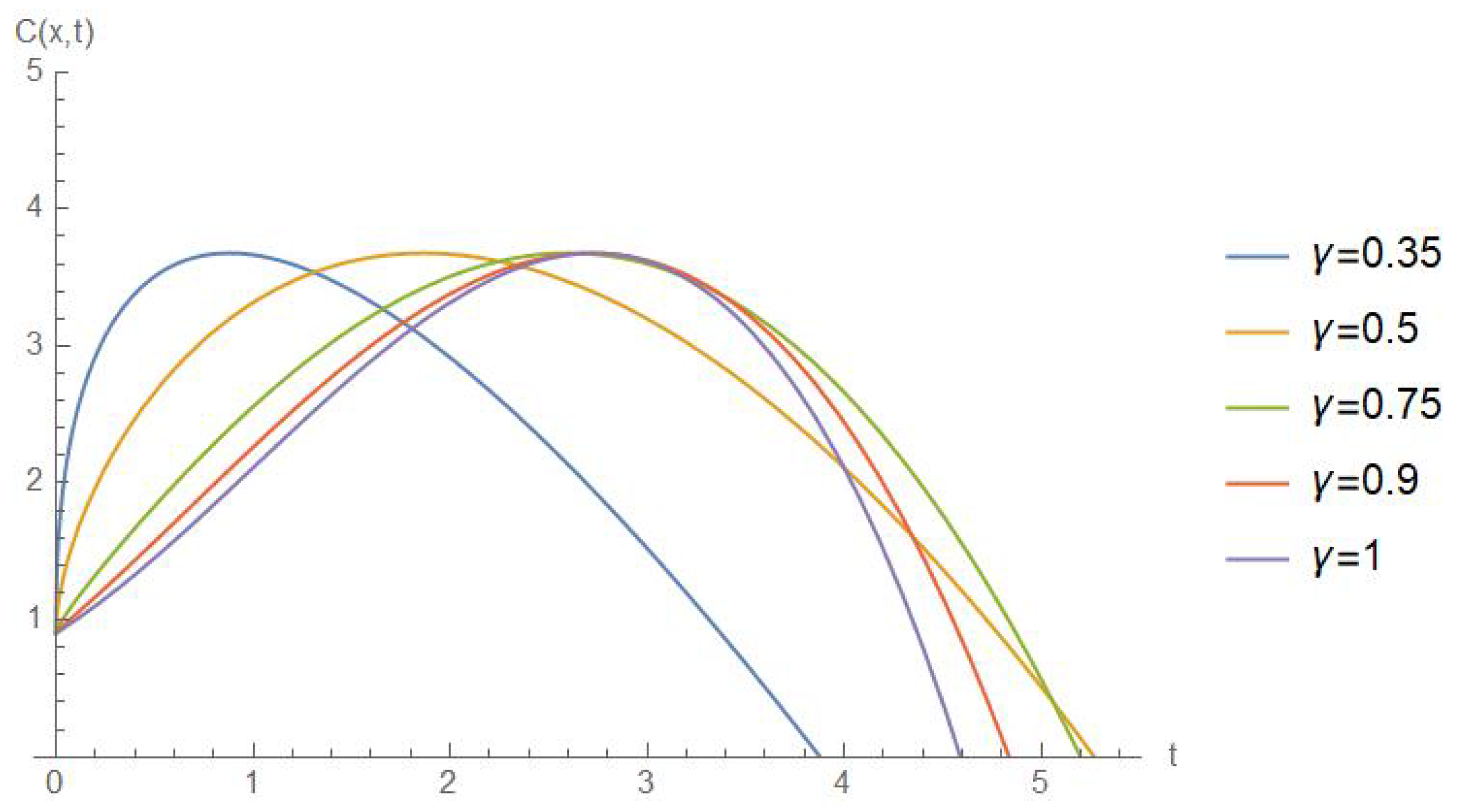
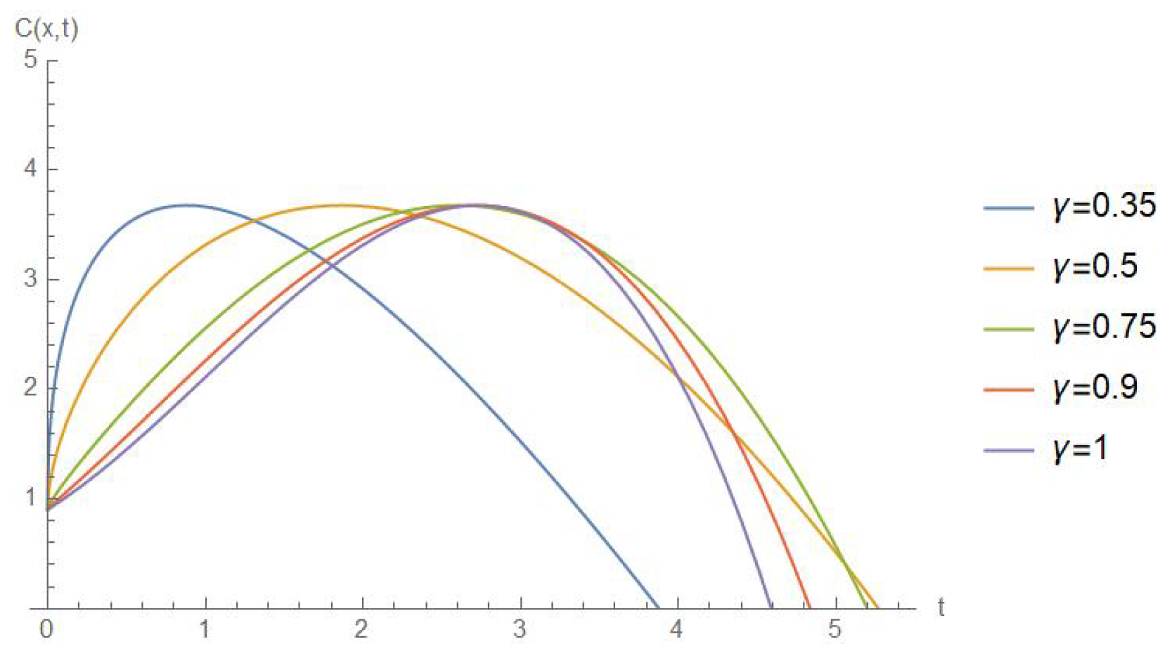
The time-dependent evolution of the cancer cell concentration for various values of the fractional order γ is depicted in a 2D format in Figure 2. These results clearly illustrate the effect of fractional order variations on the spatial distribution and temporal behavior of cancer cell concentrations. As γ changes, the concentration profile evolves differently, highlighting the critical role of the fractional order in modulating the spread and concentration of cancer cells over time.
Case II:
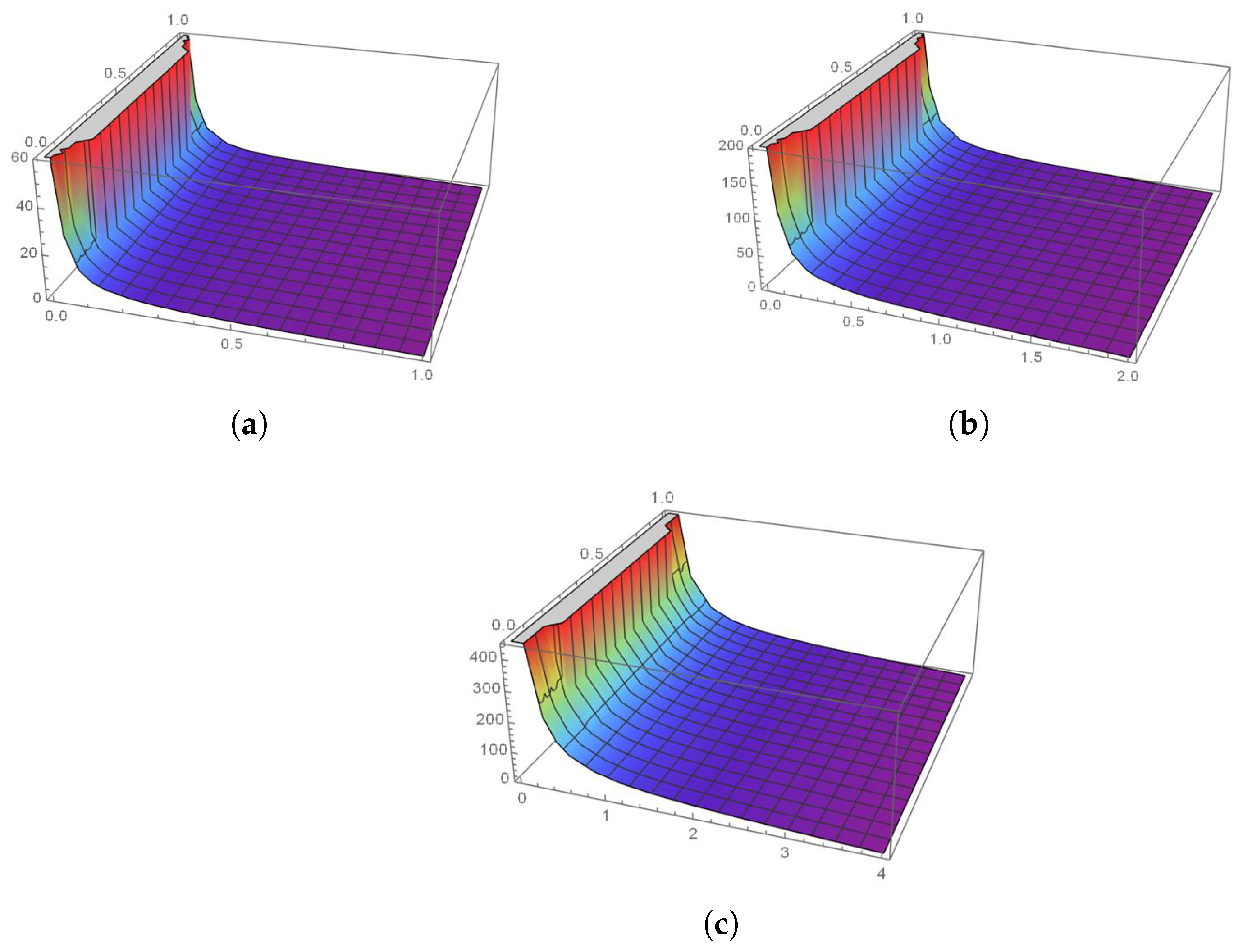
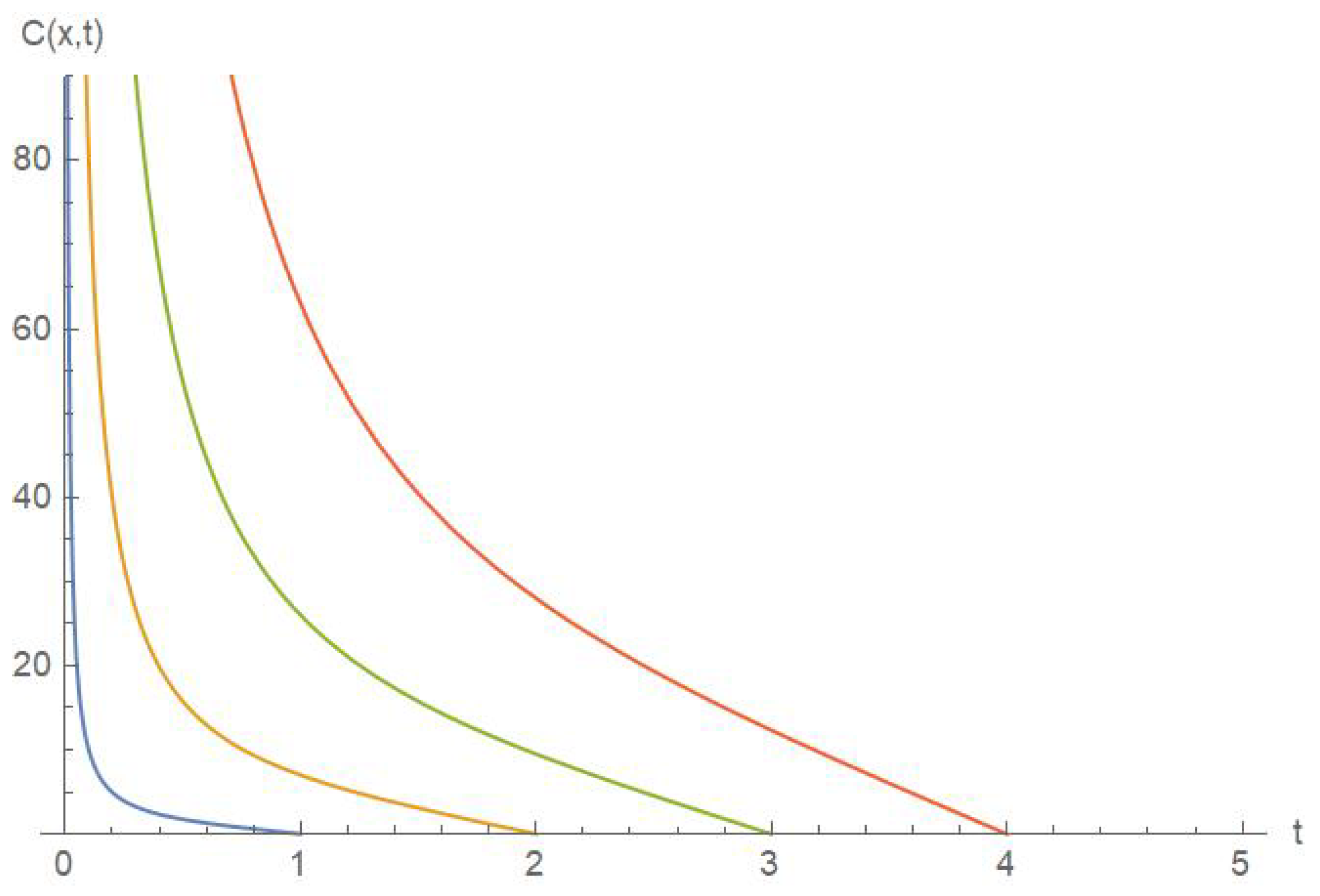
In this case, the approximate solution is independent of the fractional derivative, with its behavior relying solely on the spatial variable x. The solution is presented for specific choices of the coefficients a and b. Under these conditions, the cancer cell concentration ultimately tends toward zero, as shown in Figure 3 and Figure 4. This result emphasizes the absence of any dynamical dependence on the fractional order in this scenario, demonstrating that the concentration decay is driven solely by the spatial parameters a and b rather than the fractional dynamics. As x represents the spatial location within the tumor, approaching zero could signify the tumor core or center. In this region, the cancer cells may experience limited growth due to some factors, such as nutrient depletion, low oxygen levels, or other forms of cell death, which occur in the tumor’s inner regions. The model captures this behavior, indicating that the growth rate reduces or approaches zero at the tumor core, consistent with experimental observations of limited proliferation in the center of tumors.
Case III:
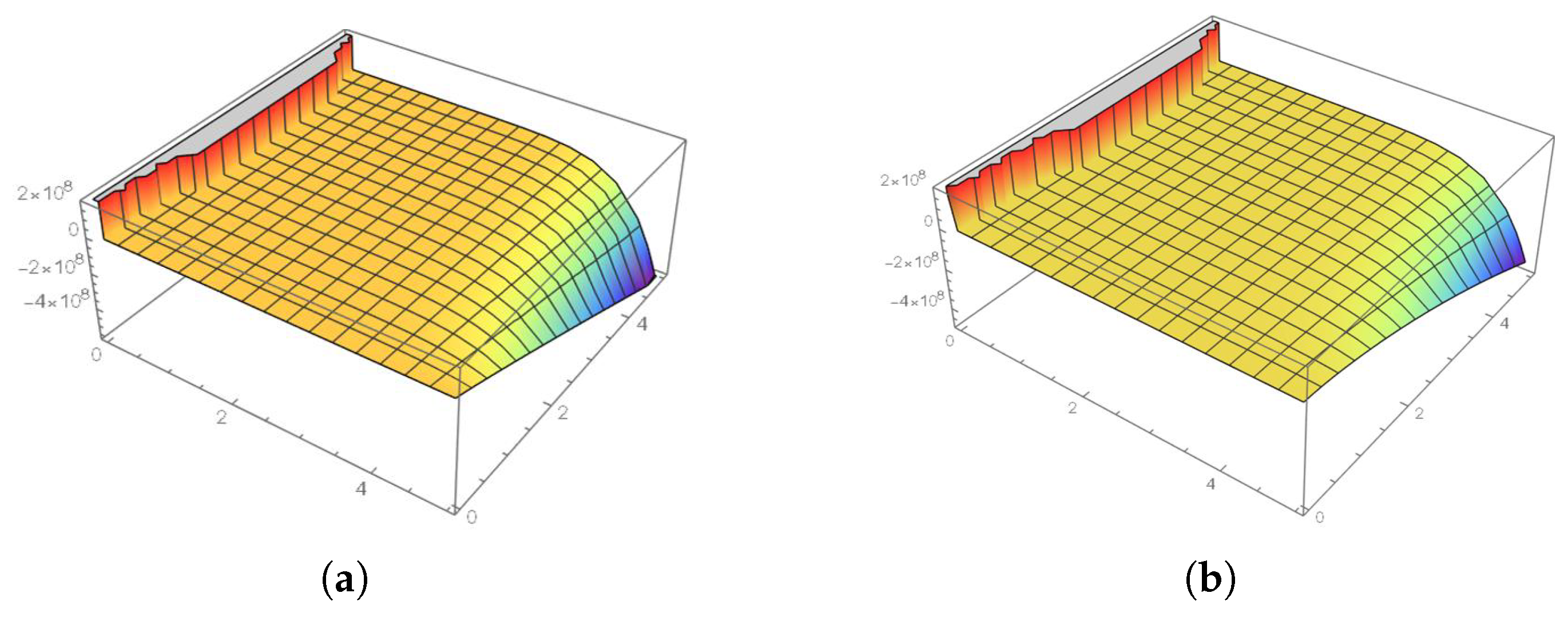
The temporal variations in cancer cell concentration for different fractional order values are shown in a 3D and 2D format in Figure 5 and Figure 6 respectively. These results provide valuable insights into how the fractional order affects the dynamic behavior of cancer cell concentration over time. The influence of the conformable fractional derivative becomes remarkable on the dynamics of the system, with the concentration profiles exhibiting distinct patterns depending on the value of γ , where smaller values of γ lead to more gradual variations in concentration, while larger values of γ result in sharper transitions and more pronounced changes in the concentration distribution over time. This case underscores the importance of the fractional order in shaping the system’s evolution and offers a deeper understanding of its role in the dynamics of cancer cell spread.
In summary, the graphical representations for each case serve as a powerful tool for understanding the complex relationship between the fractional order and cancer cell concentration dynamics. By varying the fractional order γ , we observe significant changes in the temporal and spatial evolution of the concentration profiles, highlighting the crucial role of the conformable fractional operator in influencing the system’s behavior. These results underscore the potential of fractional calculus in modeling and understanding complex biological processes, such as the spread of cancer cells.

6. Conclusions

This study presents a pioneering approach to modeling cancer tumor dynamics within a fractional framework, incorporating time-dependent, position-dependent, and concentration-dependent net killing rates. By applying the RPSM to solve these time-fractional cancer models, we introduce a highly effective technique that overcomes the challenges faced by traditional methods, such as perturbations, complex simplifications, discretization issues, and restrictive assumptions. The RPSM not only provides exact analytical solutions via a convergence series but also offers reliable numerical approximations, making it an invaluable tool for simulating fractional-order differential models. The graphical results demonstrate the method’s ability to yield accurate solutions across diverse scenarios, showcasing its versatility and robustness.
The findings highlight RPSM’s potential to revolutionize cancer modeling by offering a more nuanced and precise understanding of tumor dynamics. This approach opens new avenues for optimizing cancer treatment strategies and facilitating personalized and targeted therapies. Beyond cancer, the RPSM is promising for enhancing disease modeling in infectious diseases and epidemics, enabling more effective treatment protocols and parameter analysis.
Despite its advantages, this study acknowledges several limitations, including simplified assumptions and model parameters that may not fully capture the complexity of real-world tumor environments. However, introducing the RPSM marks a significant step forward in fractional modeling, offering theoretical and practical applications. Our work extends existing models by incorporating memory and hereditary effects, providing a more accurate representation of tumor behavior than traditional models.
Future research could further refine the model by including complex tumor behaviors like immune system interactions and angiogenesis and exploring time-space fractional derivatives for more precise spatiotemporal modeling. Additionally, integrating experimental data and clinical trial results will be essential for validating and optimizing the model, ultimately enhancing its applicability in personalized medicine. With these advancements, the RPSM-based framework has the potential to drive significant progress in cancer research and treatment.

Author Contributions

Conceptualization, H.G. and H.J.; methodology, H.G. and H.J.; investigation, H.G. and H.J.; resources, H.G.; writing—original draft preparation, H.G. and H.J.; writing—review and editing, H.G. and H.J. All authors have read and agreed to the published version of this manuscript.

Funding

This research received no external funding.

Data Availability Statement

The original contributions presented in this study are included in the article. Further inquiries can be directed to the corresponding author.

Acknowledgments

The authors thank the associate editor and anonymous referees for their insightful comments that improved the final version of this paper.

Conflicts of Interest

The authors declare no conflicts of interest.

Abbreviations

The following abbreviations are used in this manuscript:
RPSMResidual Power Series Method
PDEpartial differential equation
FPSfractional power series
PSpower series

References

  1. Benzekry, S.; Lamont, C.; Beheshti, A.; Tracz, A.; Ebos, J.M.L.; Hlatky, L.; Hahnfeldt, P. Classical mathematical models for description and prediction of experimental tumor growth. PLoS Comput. Biol. 2014, 10, e1003800. [Google Scholar] [CrossRef] [PubMed]
  2. Arshad, S.; Sohail, A.; Javed, S. Dynamical study of fractional order tumor model. Int. J. Comput. Methods 2015, 12, 1550032. [Google Scholar] [CrossRef]
  3. Kumar, S.; Kumar, A.; Samet, B.; Gómez-Aguilar, J.F.; Osman, M.S. A chaos study of tumor and effector cells in fractional tumor-immune model for cancer treatment. Chaos Solitons Fractals 2020, 141, 110321. [Google Scholar] [CrossRef]
  4. Naik, P.A.; Zu, J.; Naik, M. Stability analysis of a fractional-order cancer model with chaotic dynamics. Int. J. Biomath. 2021, 14, 2150046. [Google Scholar] [CrossRef]
  5. Naik, P.A.; Owolabi, K.M.; Yavuz, M.; Zu, J. Chaotic dynamics of a fractional order HIV-1 model involving AIDS-related cancer cells. Chaos Solitons Fractals 2020, 140, 110272. [Google Scholar] [CrossRef]
  6. Debbouche, N.; Ouannas, A.; Grassi, G.; Al-Hussein, A.B.A.; Tahir, F.R.; Saad, K.M.; Jahanshahi, H.; Aly, A.A. Chaos in cancer tumor growth model with commensurate and incommensurate fractional-order derivatives. Comput. Math. Methods Med. 2022, 2022, 5227503. [Google Scholar] [CrossRef]
  7. Qayyum, M.; Tahir, A. Mathematical Modeling of Cancer Tumor Dynamics with Multiple Fuzzification Approaches in Fractional Environment; Springer International Publishing: Cham, Switzerland, 2023. [Google Scholar]
  8. Sweilam, N.; Al-Mekhlafi, S.; Ahmed, A.; Alsheri, A.; Abo-Eldahab, E. Numerical treatments for crossover cancer model of hybrid variable-order fractional derivatives. Comput. Model Eng. Sci. 2024, 140, 1619–1645. [Google Scholar] [CrossRef]
  9. Nabil, H.; Hamaizia, T. A three-dimensional discrete fractional-order HIV-1 model related to cancer cells, dynamical analysis and chaos control. Math. Model. Numer. Simul. Appl. 2024, 4, 256–279. [Google Scholar] [CrossRef]
  10. Delgado Moya, E.M.; Rodriguez, R.A.; Pietrus, A. A mathematical model for the study of HIV/AIDS transmission with PrEP coverage increase and parameter estimation using MCMC with a Bayesian approach. Bull. Biomath. 2024, 2, 218–244. [Google Scholar] [CrossRef]
  11. Burgess, P.K.; Kulesa, P.M.; Murray, J.D.; Alroid, E.C. The interaction of growth rates and diffusion coefficients in a three dimensional mathematical model of gliomas. J. Neuropathol. Exp. Neurol. 1997, 56, 704–713. [Google Scholar] [CrossRef]
  12. Moyo, S.; Leach, P.G.L. Symmetry methods applied to a mathematical model of a tumour of the brain. Proc. Inst. Math. NAS Ukr. 2004, 50, 204–210. [Google Scholar]
  13. Sabir, Z.; Dirani, S.; Bou Saleh, S.; Mabsout, M.K.; Arbi, A. A Novel Radial Basis and Sigmoid Neural Network Combination to Solve the Human Immunodeficiency Virus System in Cancer Patients. Mathematics 2024, 12, 2490. [Google Scholar] [CrossRef]
  14. Jawad, S.; Winter, M.; Rahman, Z.-A.S.A.; Al-Yasir, Y.I.A.; Zeb, A. Dynamical Behavior of a Cancer Growth Model with Chemotherapy and Boosting of the Immune System. Mathematics 2023, 11, 406. [Google Scholar] [CrossRef]
  15. Joshi, H. Mechanistic insights of COVID-19 dynamics by considering the influence of neurodegeneration and memory trace. Phys. Scr. 2024, 99, 035254. [Google Scholar] [CrossRef]
  16. Pham, H. Mathematical Modeling the Time-Delay Interactions between Tumor Viruses and the Immune System with the Effects of Chemotherapy and Autoimmune Diseases. Mathematics 2022, 10, 756. [Google Scholar] [CrossRef]
  17. Rihan, F.A.; Rajivganthi, C. Dynamics of Tumor-Immune System with Random Noise. Mathematics 2021, 9, 2707. [Google Scholar] [CrossRef]
  18. Farman, M.; Akgül, A.; Ahmad, A.; Imtiaz, S. Analysis and dynamical behavior of fractional-order cancer model with vaccine strategy. Math. Methods Appl. Sci. 2020, 43, 4871–4882. [Google Scholar] [CrossRef]
  19. Uçar, E.; Özdemir, N. A fractional model of cancer-immune system with Caputo and Caputo-Fabrizio derivatives. Eur. Phys. J. Plus. 2021, 136, 43. [Google Scholar] [CrossRef]
  20. Uçar, S.; Koca, I.; Özdemir, N.; İnci, T. A stochastic approach to tumor modeling incorporating macrophages. Bull. Biomath. 2024, 2, 162–181. [Google Scholar] [CrossRef]
  21. Barbosa, M.A.G.; Xavier, C.P.R.; Pereira, R.F.; Petrikaite, V.; Vasconcelos, M.H. 3D cell culture models as recapitulators of the tumor microenvironment for the screening of anti-cancer drugs. Cancers 2021, 14, 190. [Google Scholar] [CrossRef] [PubMed]
  22. Özköse, F.; Yilmaz, S.; Yavuz, M.; Öztürk, I.; Senel, M.T.; Bagci, B.S.; Dogan, M.; Önal, O. A fractional modeling of tumor-immune system interaction related to lung cancer with real data. Eur. Phys. J. Plus 2021, 137, 40. [Google Scholar] [CrossRef]
  23. Özköse, F.; Yılmaz, S.; Şenel, M.T.; Yavuz, M.; Townley, S.; Sarıkaya, M.D. A mathematical modeling of patient-derived lung cancer stem cells with fractional-order derivative. Phys. Scr. 2024, 99, 115235. [Google Scholar] [CrossRef]
  24. Kalal, V.; Jha, B.K. A Kernelized Classification Approach for Cancer Recognition Using Markovian Analysis of DNA Structure Patterns as Feature Mining. Cell Biochem. Biophys. 2024, 82, 2249–2274. [Google Scholar] [CrossRef]
  25. Kalal, V.; Jha, B.K. Cancer detection with various classification models: A comprehensive feature analysis using HMM to extract a nucleotide pattern. Comput. Biol. Chem. 2024, 113, 108215. [Google Scholar] [CrossRef]
  26. Mustapha, U.T.; Ado, A.; Yusuf, A.; Qureshi, S.; Musa, S.S. Mathematical dynamics for HIV infections with public awareness and viral load detectability. Math. Model. Numer. Simul. Appl. 2023, 3, 256–280. [Google Scholar] [CrossRef]
  27. Raeisi, E.; Yavuz, M.; Khosravifarsani, M.; Fadaei, Y. Mathematical modeling of interactions between colon cancer and immune system with a deep learning algorithm. Eur. Phys. J. Plus 2024, 139, 345. [Google Scholar] [CrossRef]
  28. Keshavarz, M.; Qahremani, E.; Allahviranloo, T. Solving a fuzzy fractional diffusion model for cancer tumor by using fuzzy transforms. Fuzzy Sets Syst. 2022, 443, 198–220. [Google Scholar] [CrossRef]
  29. De Luca, P.; Marcellino, L. Conservation Law Analysis in Numerical Schema for a Tumor Angiogenesis PDE System. Mathematics 2025, 13, 28. [Google Scholar] [CrossRef]
  30. Shah, K.; Joshi, H. EOQ model for deteriorating items with fuzzy demand and finite horizon under inflation effects. Discret. Contin. Dyn. Syst.-S 2024. [Google Scholar] [CrossRef]
  31. Shen, J.; Tu, X.; Li, Y. Mathematical Modeling Reveals Mechanisms of Cancer-Immune Interactions Underlying Hepatocellular Carcinoma Development. Mathematics 2023, 11, 4261. [Google Scholar] [CrossRef]
  32. Naeem, A.; Anees, T.; Khalil, M.; Zahra, K.; Naqvi, R.A.; Lee, S.-W. SNC_Net: Skin Cancer Detection by Integrating Handcrafted and Deep Learning-Based Features Using Dermoscopy Images. Mathematics 2024, 12, 1030. [Google Scholar] [CrossRef]
  33. Rodrigues, J.A. Using Physics-Informed Neural Networks (PINNs) for Tumor Cell Growth Modeling. Mathematics 2024, 12, 1195. [Google Scholar] [CrossRef]
  34. Joshi, H.; Yavuz, M.; Taylan, O.; Alkabaa, A. Dynamic analysis of fractal-fractional cancer model under chemotherapy drug with generalized Mittag-Leffler kernel. Comput. Methods Programs Biomed. 2024, 260, 108565. [Google Scholar] [CrossRef]
  35. Ali, S.M.; Bokhari, A.H.; Yousuf, M.; Zaman, F.D. A spherically symmetric model for the tumor growth. J. Appl. Math. 2014, 726837. [Google Scholar] [CrossRef]
  36. Bokhari, A.H.; Kara, A.H.; Zaman, F.D. On the solutions and conservation laws of the model for tumor growth in the brain. J. Math. Anal. Appl. 2009, 350, 256–261. [Google Scholar] [CrossRef]
  37. Iyiola, O.S.; Zaman, F.D. A fractional diffusion equation model for cancer tumor. AIP Adv. 2014, 4, 107121. [Google Scholar] [CrossRef]
  38. Qayyum, M.; Afzal, S.; Ahmad, E.; Riaz, M.B. Fractional modeling and analysis of unsteady squeezing flow of Casson nanofluid via extended He-Laplace algorithm in Liouville-Caputo sense. Alex. Eng. J. 2023, 7, 579–591. [Google Scholar] [CrossRef]
  39. Caputo, M.; Fabrizio, M. A new definition of fractional derivative without singular kernel. Prog. Fract. Differ. Appl. 2015, 1, 73–85. [Google Scholar]
  40. Atangana, A.; Gómez-Aguilar, J.F. Decolonisation of fractional calculus rules: Breaking commutativity and associativity to capture more natural phenomena. Eur. Phys. J. Plus 2018, 133, 166. [Google Scholar] [CrossRef]
  41. Khalil, R.; Al Horani, M.; Yousef, A.; Sababheh, M. A new definition of fractional derivative. J. Comput. Appl. Math. 2014, 264, 65–70. [Google Scholar] [CrossRef]
  42. Tansri, K.; Kittisopaporn, A.; Chansangiam, P. Numerical solutions of the space-time fractional diffusion equation via a gradient-descent iterative procedure. J. Math. Comput. Sci 2023, 31, 353–366. [Google Scholar] [CrossRef]
  43. Korpinar, Z.; Inc, M.; Hinça, E.; Baleanu, D. Residual power series algorithm for fractional cancer tumor models. Alex. Eng. J. 2020, 59, 1405–1412. [Google Scholar] [CrossRef]
  44. Ghanbari, B.; Kumar, S.; Kumar, R. A study of behaviour for immune and tumor cells in immunogenetic tumour model with non-singular fractional derivative. Chaos Solitons Fractals 2020, 133, 109619. [Google Scholar] [CrossRef]
  45. Arfan, M.; Shah, K.; Ullah, A.; Shutaywi, M.; Kumam, P.; Shah, Z. On fractional order model of tumor dynamics with drug interventions under nonlocal fractional derivative. Results Phys. 2021, 21, 103783. [Google Scholar] [CrossRef]
  46. Ahmad, S.; Ullah, A.; Akgül, A.; Baleanu, D. Theoretical and numerical analysis of fractal fractional model of tumor-immune interaction with two different kernels. Alex. Eng. J. 2022, 61, 5735–5752. [Google Scholar] [CrossRef]
  47. Feng, Z. The first-integral method to study the Burgers-Korteweg-de Vries equation. J. Phys. A Math. Gen. 2002, 35, 343. [Google Scholar] [CrossRef]
  48. Abuasad, S.; Hashim, I.; Abdul-Karim, S.A. Modified fractional reduced differential transform method for the solution of multiterm time-fractional diffusion equations. Adv. Math. Phys. 2019, 2019, 5703916. [Google Scholar] [CrossRef]
  49. Prakash, A.; Veeresha, P.; Prakasha, D.G.; Goyal, M. A new efficient technique for solving fractional coupled Navier-Stokes equations using q-homotopy analysis transform method. Pramana 2019, 93, 6. [Google Scholar] [CrossRef]
  50. Shah, R.; El-Zahar, N.A.; Akgül, E.R.; Khan, A.; Kafle, J. Analysis of Fractional-Order Regularized Long-Wave Models via a Novel Transform. J. Funct. Spaces 2022, 2022, 2754507. [Google Scholar] [CrossRef]
  51. Zidan, A.M.; Khan, A.; Shah, R.; Alaoui, M.K.; Weera, W. Evaluation of time-fractional Fisher’s equations with the help of analytical methods. AIMS Math. 2022, 7, 18746–18766. [Google Scholar] [CrossRef]
  52. Botmart, T.; Agarwal, R.P.; Naeem, M.; Khan, A.; Shah, R. On the solution of fractional modified Boussinesq and approximate long wave equations with non-singular kernel operators. AIMS Math. 2022, 7, 12483–12513. [Google Scholar] [CrossRef]
  53. Alderremy, A.A.; Aly, S.; Fayyaz, R.; Khan, A.; Shah, R.; Wyal, N. The analysis of fractional-order nonlinear systems of third order KdV and Burgers equations via a novel transform. Complexity 2022, 2022, 4935809. [Google Scholar] [CrossRef]
  54. Chen, L.; Liu, Q. Local fractional homotopy perturbation method for solving coupled sine-Gordon equations in fractal domain. Fractal Fract. 2022, 6, 404. [Google Scholar] [CrossRef]
  55. Gündoǧdu, H.; Gözükızıl, Ö.F. On the approximate numerical solutions of the fractional heat equation with heat source and heat loss. Therm. Sci. 2022, 26, 3773–3786. [Google Scholar] [CrossRef]
  56. El-Ajou, A.; Abu-Arqub, O.; Al-Zhour, Z.; Momani, S. New results on fractional power series: Theories and applications. Entropy 2013, 15, 5305–5323. [Google Scholar] [CrossRef]
  57. Az-Zo’bi, E.A. Exact analytic solutions for nonlinear diffusion equations via generalized residual power series method. Int. J. Math. Comput. Sci. 2019, 14, 69–78. [Google Scholar]
  58. Guo, T.; Nikan, O.; Avazzadeh, Z. Efficient alternating direction implicit numerical approaches for multi-dimensional distributed-order fractional integro differential problems. Comp. Appl. Math. 2022, 41, 236. [Google Scholar] [CrossRef]
  59. Gillani, R.; Dawar, A.; Khan, H. The improved residual power series method for the solutions of higher-order linear and nonlinear boundary value problems. J. Umm Al-Qura Univ. Appl. Sci. 2024. [Google Scholar] [CrossRef]
  60. Kittipoom, P. Extracting explicit coefficient formulas: A robust approach to the Laplace residual power series method. Alex. Eng. J. 2024, 109, 1–11. [Google Scholar] [CrossRef]
  61. Zhang, J.; Tian, X. Laplace-residual power series method for solving fractional generalized long wave equations. Ocean Eng. 2024, 310, 118693. [Google Scholar] [CrossRef]
  62. El-Ajou, A.; Arqub, O.A.; Momani, S. Approximate analytical solution of the nonlinear fractional KdV-Burgers equation: A new iterative algorithm. J. Comput. Phys. 2015, 293, 81–95. [Google Scholar] [CrossRef]
Figure 1. The surface plots of the approximate solution of Case I for γ = (a) 0.4, (b) 0.6, (c) 0.8, and (d) 0.95 , respectively.
Mathematics 13 00536 g001
Figure 2. The concentration of cancer cells in Case I.
Mathematics 13 00536 g002
Figure 3. The surface plots of the approximate solution of Case II for (a) a = b , ( b ) a = 8 b , and (c) a = 27 b , respectively.
Mathematics 13 00536 g003
Figure 4. The concentration of cancer cells in Case II for specific values of a and b.
Mathematics 13 00536 g004
Figure 5. The surface plots of the approximate solution of Case III for γ = (a) 0.35, (b) 0.5, (c) 0.95, (d) 1.25, (e) 1.6, and (f) 1.95 , respectively.
Mathematics 13 00536 g005aMathematics 13 00536 g005b
Figure 6. The concentration of cancer cells in Case III.
Mathematics 13 00536 g006
Disclaimer/Publisher’s Note: The statements, opinions and data contained in all publications are solely those of the individual author(s) and contributor(s) and not of MDPI and/or the editor(s). MDPI and/or the editor(s) disclaim responsibility for any injury to people or property resulting from any ideas, methods, instructions or products referred to in the content.