Enhanced Multilinear PCA for Efficient Image Analysis and Dimensionality Reduction: Unlocking the Potential of Complex Image Data

Abstract

This paper presents an Enhanced Multilinear Principal Component Analysis (EMPCA) algorithm, an improved variant of the traditional Multilinear Principal Component Analysis (MPCA) tailored for efficient dimensionality reduction in high-dimensional data, particularly in image analysis tasks. EMPCA integrates random singular value decomposition to reduce computational complexity while maintaining data integrity. Additionally, it innovatively combines the dimensionality reduction method with the Mask R-CNN algorithm, enhancing the accuracy of image segmentation. Leveraging tensors, EMPCA achieves dimensionality reduction that specifically benefits image classification, face recognition, and image segmentation. The experimental results demonstrate a 17.7% reduction in computation time compared to conventional methods, without compromising accuracy. In image classification and face recognition experiments, EMPCA significantly enhances classifier efficiency, achieving comparable or superior accuracy to algorithms such as Support Vector Machines (SVMs). Additionally, EMPCA preprocessing exploits latent information within tensor structures, leading to improved segmentation performance. The proposed EMPCA algorithm holds promise for reducing image analysis runtimes and advancing rapid image processing techniques.

1. Introduction

With the continuous advancement of big data and storage technologies, vast amounts of high-dimensional and multi-dimensional data are generated daily. Tensors, which are multi-dimensional arrays, extend the concepts of vectors and matrices. Their application is widespread; for instance, in computer vision, colored images and grayscale videos are represented as third-order tensor data, while colored videos are considered fourth-order tensor data. In traditional data analysis, which primarily uses vector and matrix representations and operations, multi-order data are often “unfolded” into matrices for processing.

Principal Component Analysis (PCA) [1] is a widely used unsupervised technique for dimensionality reduction and feature extraction. It transforms high-dimensional data into a lower-dimensional representation through linear transformations, while preserving as much of the original information as possible. Bansal and Chawla introduced Normalized Principal Component Analysis [2], which enhances the dimensionality reduction process by using singular value decomposition instead of eigenvalue decomposition, thereby normalizing the images. In addition, 2D-PCA [3] identifies a set of orthogonal projection vectors by performing eigenvalue decomposition on the covariance matrix of the sample data, thereby maximizing the variance of the projected data. Independent Component Analysis (ICA) [4] is a statistical technique aimed at extracting independent components from mixed signals by estimating a linear transformation matrix.

Kernel Principal Component Analysis (KPCA) [5] is a nonlinear method that maps the original data into a high-dimensional feature space. In this transformed space, the data become linearly separable, which facilitates dimensionality reduction and feature extraction for nonlinear datasets. Linear Discriminant Analysis (LDA) [6], on the other hand, is a commonly used supervised learning method that maps data to a lower-dimensional space by identifying an optimal projection direction. The key objective of LDA is to maximize the separability between different classes of data. However, in the vectorization or matrixization process of the above methods, the multilinear structure of the data is lost, resulting in suboptimal processing performance. Therefore, research on high-dimensional tensor data is necessary.

Kolda and Bader [7] introduced the fundamental theory and methods of tensor decomposition. Among these, Higher Order Singular Value Decomposition (HOSVD) is a generalization of traditional singular value decomposition designed for processing high-dimensional data. Unlike two-dimensional matrices, tensors are multi-dimensional arrays that encapsulate data from multiple modes. HOSVD decomposes such multi-dimensional data into a set of mode-specific matrices, thereby facilitating a better understanding of the data’s structure and interrelationships.

The applications of tensor decomposition span various fields. Fahad et al. [8] applied low-rank tensor decomposition in unconventional reservoir petroleum engineering to tackle challenges such as large dataset management and missing data imputation. Gao et al. [9] proposed an unsupervised dimensionality reduction method based on tensor-based low-rank collaborative graph embedding, applying it to high-spectral datasets of bile duct cancer under a microscope, with experimental results confirming the effectiveness of the algorithm. Xie et al. [10] used Higher Order Singular Value Decomposition of tensors to predict short-term traffic flow on highways. Their experimental results demonstrated that HOSVD captured the periodicity, multimodality, and integrity of traffic flow data, reducing fluctuations and randomness, and thus improving the accuracy of the model. Yin et al. [11] proposed a dimensionality reduction technique called Regularized Non-negative Tensor Factorization on hypergraphs to uncover the nonlinear structure in high-dimensional data. Experimental results on synthetic manifolds, real-world image datasets, and electroencephalogram signals validated the effectiveness of this algorithm.

In tensor decomposition, a widely used algorithm is Multilinear Principal Component Analysis (MPCA), proposed by Lu et al. [12], which extends traditional Principal Component Analysis to multidimensional cases. Unlike conventional PCA algorithms that employ linear transformations for dimensionality reduction, MPCA is designed for data with multiple modes or features. Lu et al. applied MPCA to gait recognition, and their experimental results demonstrated that the MPCA algorithm can simultaneously account for the correlations between different modes, thereby capturing more comprehensive information in multidimensional datasets. Block-based Multilinear Principal Component Analysis [13] divides tensors into multiple blocks and conducts experiments on facial recognition and gait recognition datasets, showing its capability to handle large-scale datasets with reduced runtime compared to traditional PCA. The Multilinear Principal Component Analysis Network [14] simulates multilinear structures by stacking multiple PCA layers, allowing for better capture of high-order features in the data.

The experimental results from the aforementioned studies indicate that the MPCA algorithm is effective in analyzing high-dimensional image data. However, in the MPCA algorithm described above, the matrix obtained after tensor unfolding is of high dimensionality, leading to high computational complexity during the subsequent singular value decomposition step. As a result, processing large-scale, high-dimensional images can be time-consuming. Existing MPCA algorithms, including their enhanced versions, have rarely been applied to image segmentation, and traditional segmentation algorithms have limited integration with tensor methods. Conventional image segmentation algorithms typically treat video frames as independent, neglecting the structural information between frames. Hence, there is a need for further research on the application of MPCA in image segmentation.

This paper proposes an improved MPCA algorithm that integrates randomized singular value decomposition to optimize computational efficiency and reduce processing time. The algorithm is then combined with Mask R-CNN to enhance the accuracy of image segmentation. The enhanced algorithm is then applied to the field of image classification. By reducing the dimensionality of high-dimensional tensors and extracting more useful features from the tensor data, the runtime of the classifier is significantly reduced without compromising, and in some cases even improving, classification accuracy. In the context of image segmentation, we introduce the EMPCA algorithm as a preprocessing step. Unlike traditional methods that preprocess individual images separately, this algorithm effectively exploits the structural information between tensors and extracts latent information, thereby enhancing the effectiveness of image segmentation.

2. Enhanced Multilinear Principal Component Analysis Algorithm

The main steps of the Enhanced Multilinear Principal Component Analysis (EMPCA) algorithm are as follows: first, the original tensor is unfolded according to each mode, and then random singular value decomposition is performed on the unfolding matrix of each mode [15]. The projection matrix is constructed from the eigenvectors corresponding to the largest eigenvalues in the left singular matrix. Then, with the objective of maximizing scatter, the projection matrix is sequentially solved and updated through alternating iterations, and finally, the reduced tensor is obtained through the projection matrix.

Compared to existing algorithms, the EMPCA algorithm focuses more on the increased computational complexity caused by high-dimensional data. Therefore, it introduces the random singular value decomposition algorithm to reduce computational complexity and accelerate the process of singular value decomposition.

2.1. Random Singular Value Decomposition Algorithm

In the MPCA algorithm, after unfolding the tensor according to modes, the classical singular value decomposition algorithm is used to obtain the top k principal components. However, for solving the top k principal components of m*n large-sized matrices, the computational complexity of the classical singular value decomposition algorithm is O(mnk), where m, n, and k are all positive integers. Considering that the dimensions of the unfolding matrices are large after tensor unfolding, if more principal components need to be retained to preserve more information, i.e., m, n, and k are large positive integers, then the classical singular value decomposition algorithm will consume a lot of time. Since the MPCA algorithm requires solving the left singular matrix multiple times, it is considered to reduce the computational complexity and runtime of the MPCA algorithm while maintaining a certain precision.

Here, the random singular value decomposition (RSVD) algorithm [16] is introduced to replace the singular value decomposition algorithm. The RSVD algorithm introduces randomness to the original matrix and uses random projection techniques to transform the original matrix into a lower-dimensional subspace. Then, singular value decomposition is performed in this subspace, reducing the computational complexity while retaining the main singular values and corresponding singular vectors.

The RSVD algorithm is an approximate method for efficiently computing matrix singular value decomposition. It reduces computational complexity and accelerates singular value decomposition by introducing random matrices and partial sample data. RSVD reduces computational complexity through random projections while preserving the main features of the data, with its results progressively approaching those of traditional SVD as the sample size increases. The detailed steps of the RSVD algorithm are as following Algorithm 1 [16]:

Algorithm 1: Random Singular Value Decomposition algorithm

$\mathrm{Input}: \mathrm{Matrix}: \mathrm{A}\in {\mathrm{R}}^{\mathrm{m}\times \mathrm{n}}$, with rank k $\mathrm{Output}: \mathrm{Decomposition} \mathrm{result}: \mathrm{U}\in {\mathrm{R}}^{\mathrm{m}\times \mathrm{k}},\mathrm{S}\in {\mathrm{R}}^{\mathrm{k}\times \mathrm{k}},\mathrm{V}\in {\mathrm{R}}^{\mathrm{n}\times \mathrm{k}}$ $\left(\mathrm{a}\right) \mathrm{Generate} \mathrm{a} \mathrm{random} \mathrm{matrix}: \mathrm{Generate} \mathrm{a} \mathrm{random} \mathrm{matrix} \mathsf{\Omega }\in {\mathrm{R}}^{\mathrm{n}\times \mathrm{k}}$ following a Gaussian distribution; (b) Matrix multiplication: Multiply the original matrix by the random matrix to obtain a projection matrix:                  $\mathrm{Y}=\mathrm{A}\mathsf{\Omega }.$                        (1) $\mathrm{This} \mathrm{step} \mathrm{can} \mathrm{be} \mathrm{achieved} \mathrm{by} \mathrm{sampling} \mathrm{the} \mathrm{original} \mathrm{matrix} \mathrm{A}$$\mathrm{with} \mathrm{a} \mathrm{random} \mathrm{matrix} \mathsf{\Omega }$; (c) Perform QR decomposition on matrix Y:                  $\mathrm{Y}=\mathrm{Q}\mathrm{R}$.                         (2) $\left(\mathrm{d}\right) \mathrm{Multiply} {\mathrm{Q}}^{\mathrm{\top }}$$\mathrm{with} \mathrm{A} \mathrm{to} \mathrm{obtain} \mathrm{a} \mathrm{new} \mathrm{matrix} \mathrm{B} \mathrm{of} \mathrm{size} \mathrm{k}\times$ n:                  $\mathrm{B}={\mathrm{Q}}^{\mathrm{\top }}\mathrm{A}$.                         (3) (e) Perform singular value decomposition on matrix B:                  $\mathrm{B}=\tilde{\mathrm{U}}\mathrm{S}{\mathrm{V}}^{\mathrm{\top }}$.                       (4)

Step e is similar to classical singular value decomposition, but since only the projection matrix needs to be operated on, the computational complexity is lower than that of the classical singular value decomposition algorithm. When the projection dimension is sufficiently large, random matrices can, with high probability, provide a very accurate low-rank approximation, close to the conventional SVD.

As an approximate algorithm for classical singular value decomposition, although the RSVD algorithm cannot provide exactly the same results as the classical singular value decomposition algorithm, its computational complexity is $\mathrm{O}\left(\mathrm{m}\mathrm{n}\mathrm{l}\mathrm{o}\mathrm{g}\right(\mathrm{k})+(\mathrm{m}+\mathrm{n}\left){\mathrm{k}}^2\right)$, which is much smaller than that of the classical singular value decomposition algorithm for high-dimensional matrices, i.e., when m, n, and k are large positive integers. Compared to the classical singular value decomposition algorithm, the RSVD algorithm greatly reduces computational complexity and can handle large datasets and high-dimensional matrices.

2.2. Multilinear Principal Component Analysis Algorithm

Principal Component Analysis (PCA) is an unsupervised dimensionality reduction technique that aims to capture the maximum variance in the original data while minimizing the reconstruction error between the original and the lower-dimensional representation. PCA is a linear method, which means that the transformation from the original data to the new low-dimensional space is achieved through a linear projection. In PCA, the original (n)-dimensional data matrix (X) is mapped to a new orthogonal space, with axes oriented along the directions of maximum variance. The features in this new orthogonal space are referred to as principal components.

For tensor data, such as color images or grayscale video sequences, the application of PCA typically involves unfolding the tensor data into high-dimensional vectors. This process disrupts the inherent structure and correlations within the tensor, leading to increased computational complexity and higher memory requirements. To address these challenges, Multilinear Principal Component Analysis (MPCA) has been developed as a dimensionality reduction technique specifically designed for tensor data, effectively preserving the natural structure while minimizing the computational and memory overhead.

The goal of Multilinear Principal Component Analysis is to find N projection matrices $\left\{{\tilde{\mathrm{U}}}^{\left(\mathrm{n}\right)}\in {\mathrm{R}}^{{\mathrm{I}}_{\mathrm{n}}\times {\mathrm{P}}_{\mathrm{n}}},{\mathrm{I}}_{\mathrm{n}}\ge {\mathrm{P}}_{\mathrm{n}},\mathrm{n}=\mathrm{1,2}\cdots ,\mathrm{N}\right\}$ to map the tensor ${\mathcal{X}}_{\mathrm{i}}\in {\mathrm{R}}^{{\mathrm{I}}_1\times {\mathrm{I}}_2\times \cdots {\mathrm{I}}_{\mathrm{N}}}$ into a lower-dimensional space ${\mathrm{R}}^{{\mathrm{P}}_1\times {\mathrm{P}}_2\times \cdots {\mathrm{P}}_{\mathrm{N}}}$, simultaneously maximizing the scatter of the new tensor [12], as shown below:

$$\left\{{\tilde{\mathrm{U}}}^{\left(\mathrm{n}\right)}\in {\mathrm{R}}^{{\mathrm{I}}_{\mathrm{n}}\times {\mathrm{P}}_{\mathrm{n}}},{\mathrm{I}}_{\mathrm{n}}\ge {\mathrm{P}}_{\mathrm{n}}\right\}=\underset{{\tilde{\mathrm{U}}}^{\left(1\right)},{\tilde{\mathrm{U}}}^{\left(2\right)},\dots ,{\tilde{\mathrm{U}}}^{\left(\mathrm{N}\right)}}{\mathrm{a}\mathrm{r}\mathrm{g}\mathrm{m}\mathrm{a}\mathrm{x}}{\mathsf{\Psi }}_{\mathrm{y}}$$

(5)

The Multilinear Principal Component Analysis algorithm sequentially solves the projection matrix through alternating iterations. It first fixes all projection matrices ${\tilde{\mathrm{U}}}^{\left(1\right)}\dots {\tilde{\mathrm{U}}}^{(\mathrm{n}-1)},{\tilde{\mathrm{U}}}^{(\mathrm{n}+1)}\dots {\tilde{\mathrm{U}}}^{\left(\mathrm{N}\right)}$ except ${\tilde{\mathrm{U}}}^{\left(\mathrm{n}\right)}$, solves ${\tilde{\mathrm{U}}}^{\left(\mathrm{n}\right)}$, then fixes the solved ${\tilde{\mathrm{U}}}^{\left(\mathrm{n}\right)}$, and solves ${\tilde{\mathrm{U}}}^{(\mathrm{n}+1)}$, and so on, continuously updating the projection matrix until convergence or reaching the maximum number of iterations.

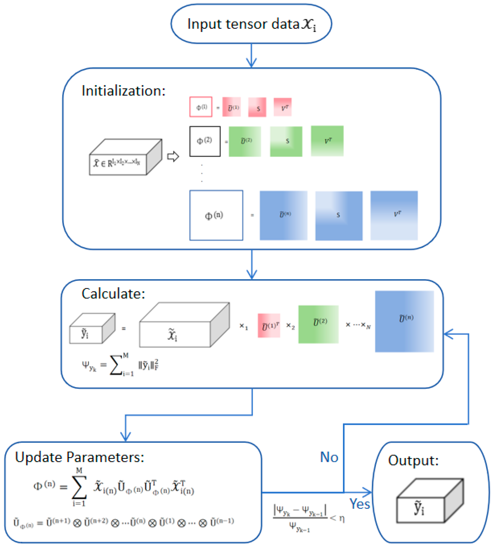
2.3. Enhanced Multilinear Principal Component Analysis Algorithm

Considering the high-dimensional nature of tensor data and the high time cost of the Multilinear Principal Component Analysis algorithm in handling high-dimensional datasets, this paper introduces the random singular value algorithm into Multilinear Principal Component Analysis to reduce computational resources and computing time while maintaining a certain precision when facing high-dimensional datasets. The convergence of EMPCA relies on the stability and convergence of RSVD, ensuring that the overall decomposition converges to a low-rank approximation solution through the iterative optimization of factor matrices. The flowchart of the EMPCA algorithm is shown in Figure 1. The detailed steps of the EMPCA algorithm are as follows in Algorithm 2.

Algorithm 2: Enhanced Multilinear Principal Component Analysis Algorithm

$\mathrm{Input}: \mathrm{Tensor} \mathrm{samples} \left\{{\mathcal{X}}_{\mathrm{i}}\in {\mathrm{R}}^{{\mathrm{I}}_1\times {\mathrm{I}}_2\times \dots \times {\mathrm{I}}_{\mathrm{N}}},\mathrm{i}=1,\dots ,\mathrm{M}\right\}$ $\mathrm{Output}: \mathrm{Reduced}-\mathrm{dimensional} \mathrm{tensor} \left\{{\tilde{\mathrm{y}}}_{\mathrm{i}}\in {\mathrm{R}}^{{\mathrm{I}}_1\times {\mathrm{I}}_2\times \dots \times {\mathrm{I}}_{\mathrm{N}}},\mathrm{i}=1,\dots ,\mathrm{M}\right\}$ $\left(\mathrm{a}\right) \mathrm{Preprocessing}: \mathrm{Centering} \mathrm{the} \mathrm{tensor} \mathrm{samples} \left\{{\mathcal{X}}_{\mathrm{i}}\in {\mathrm{R}}^{{\mathrm{I}}_1\times {\mathrm{I}}_2\times \dots \times {\mathrm{I}}_{\mathrm{N}}},\mathrm{i}=1,\dots ,\mathrm{M}\right\}$, where the mean is given by:                  $\stackrel{\mathcal{‾}}{\mathcal{X}}={\displaystyle \frac{1}{\mathrm{M}}}{\sum }_{\mathrm{i}=1}^{\mathrm{M}} {\mathcal{X}}_{\mathrm{i}}$                       (6) $(\mathrm{b}) \mathrm{Initialization}: \mathrm{Obtain} \mathrm{the} \mathrm{matrix} \mathrm{composed} \mathrm{of} \mathrm{the} \mathrm{largest} \sin \mathrm{gular} \mathrm{vectors} \mathrm{from} \mathrm{the} \mathrm{RSVD} \mathrm{decomposition}. {\mathsf{\Phi }}^{\left(\mathrm{n}\right)}={\sum }_{\mathrm{i}=1}^{\mathrm{M}} {\tilde{\mathcal{X}}}_{\mathrm{i}\left(\mathrm{n}\right)}{\tilde{\mathcal{X}}}_{\mathrm{i}\left(\mathrm{n}\right)}^{\mathrm{T}}$$. \mathrm{Form} \mathrm{the} \mathrm{matrix} {\tilde{\mathrm{U}}}^{\left(\mathrm{n}\right)}$$\mathrm{by} \mathrm{selecting} \mathrm{the} \mathrm{left} \sin \mathrm{gular} \mathrm{vectors} \mathrm{corresponding} \mathrm{to} \mathrm{the} {\mathrm{P}}_{\mathrm{n}}$ largest singular values from the left singular matrix. (c) Local Optimization: (1) The n-mode matrix product of a tensor $\mathcal{A}\in {\mathrm{R}}^{{\mathrm{I}}_1\times {\mathrm{I}}_2\times \dots \times {\mathrm{I}}_{\mathrm{N}}}$ and a matrix $\mathrm{U}\in {\mathrm{R}}^{{\mathrm{J}}_{\mathrm{n}}\times {\mathrm{I}}_{\mathrm{n}}}$ is denoted as A ${\times }_{\mathrm{n}}$U, and is defined as:                  ${\left(\mathcal{A}{\times }_{\mathrm{n}}\mathrm{U}\right)}_{{\mathrm{i}}_1\times \cdots {\mathrm{i}}_{\mathrm{n}-1}\times {\mathrm{j}}_{\mathrm{n}}\times {\mathrm{i}}_{\mathrm{N}}}={\sum }_{{\mathrm{i}}_{\mathrm{n}}=1}^{{\mathrm{I}}_{\mathrm{n}}} {\mathrm{a}}_{{\mathrm{i}}_1\times \cdots {\mathrm{i}}_{\mathrm{n}}{\mathrm{u}}_{\mathrm{j}\mathrm{n},{\mathrm{i}}_{\mathrm{n}}}}$.              (7) Compute the reduced-dimensional tensor [12]:                  $\left\{{\tilde{\mathrm{y}}}_{\mathrm{i}}={\tilde{\mathcal{X}}}_{\mathrm{i}}{\times }_1{\tilde{\mathrm{U}}}^{(1{)}^{\mathrm{T}}}\times \cdots {\times }_{\mathrm{N}}{\tilde{\mathrm{U}}}^{(\mathrm{N}{)}^{\mathrm{T}}},\mathrm{i}=\mathrm{1,2},\cdots \mathrm{M}\right\}$           (8) (2) Calculate the scatter:                  ${\mathsf{\Psi }}_{{\mathrm{y}}_{\mathrm{k}}}=\sum _{\mathrm{i}=1}^{\mathrm{M}} {∥{\tilde{\mathrm{y}}}_{\mathrm{i}}∥}_{\mathrm{F}}^2$                      (9) (3) Iterate the following steps: (3.1) For each, perform RSVD decomposition, and obtain the matrix composed of the largest singular vectors from the left singular matrix. Additional parameters are (“$\otimes$” represents the Kronecker product of matrices) [12]:                  ${\mathsf{\Phi }}^{\left(\mathrm{n}\right)}=\sum _{\mathrm{i}=1}^{\mathrm{M}} {\tilde{\mathcal{X}}}_{\mathrm{i}\left(\mathrm{n}\right)}{\tilde{\mathrm{U}}}_{{\mathsf{\Phi }}^{\left(\mathrm{n}\right)}}{\tilde{\mathrm{U}}}_{{\mathsf{\Phi }}^{\left(\mathrm{n}\right)}}^{\mathrm{T}}{\tilde{\mathcal{X}}}_{\mathrm{i}\left(\mathrm{n}\right)}^{\mathrm{T}}$                (10)                ${\tilde{\mathrm{U}}}_{{\mathsf{\Phi }}^{\left(\mathrm{n}\right)}}={\tilde{\mathrm{U}}}^{(\mathrm{n}+1)}\otimes {\tilde{\mathrm{U}}}^{(\mathrm{n}+2)}\otimes \cdots {\tilde{\mathrm{U}}}^{\left(\mathrm{n}\right)}\otimes {\tilde{\mathrm{U}}}^{\left(1\right)}\otimes \cdots \otimes {\tilde{\mathrm{U}}}^{(\mathrm{n}-1)}$          (11) (3.2) Compute the reduced-dimensional tensor and scatter:                  $\left\{{\tilde{\mathrm{y}}}_{\mathrm{i}}={\tilde{\mathcal{X}}}_{\mathrm{i}}{\times }_1{\tilde{\mathrm{U}}}^{(1{)}^{\mathrm{T}}}\times \cdots {\times }_{\mathrm{N}}{\tilde{\mathrm{U}}}^{(\mathrm{N}{)}^{\mathrm{T}}},\mathrm{i}=\mathrm{1,2},\cdots \mathrm{M}\right\}$           (12)                  ${\mathsf{\Psi }}_{{\mathrm{y}}_{\mathrm{k}}}=\sum _{\mathrm{i}=1}^{\mathrm{M}} {∥{\tilde{\mathrm{y}}}_{\mathrm{i}}∥}_{\mathrm{F}}^2$                      (13) (3.3) Stop when the condition becomes true:                  ${\displaystyle \frac{\left|{\mathsf{\Psi }}_{{\mathrm{y}}_{\mathrm{k}}}-{\mathsf{\Psi }}_{{\mathrm{y}}_{\mathrm{k}-1}}\right|}{{\mathsf{\Psi }}_{{\mathrm{y}}_{\mathrm{k}-1}}}}<\mathsf{\eta }$                      (14) (d) Projection: Obtain the final reduced-dimensional tensor:                  $\left\{{\tilde{\mathrm{y}}}_{\mathrm{i}}={\tilde{\mathcal{X}}}_{\mathrm{i}}{\times }_1{\tilde{\mathrm{U}}}^{(1{)}^7}{\times }_2{\tilde{\mathrm{U}}}^{(2{)}^{\mathrm{T}}}\times \cdots \times {}_{\mathrm{N}}\tilde{\mathrm{U}}^{(\mathrm{N}{)}^{\mathrm{T}}}\right\}$               (15)

2.4. Algorithm Performance Experiment and Specific Analysis Metrics

2.4.1. Metrics

In this context, the relative error is introduced to measure the relative difference between the reconstructed result and the original tensor, referred to as the reconstruction error. The reconstruction error is defined as follows:$\mathrm{R}\mathrm{E}={\displaystyle \frac{\parallel \stackrel{\mathcal{ˆ}}{\mathcal{X}}-\mathcal{X}{\parallel }_{\mathrm{F}}}{\parallel \mathcal{X}{\parallel }_{\mathrm{F}}}}$, where RR represents the Reserved Rate. The Reserved Rate is calculated as $\mathrm{R}\mathrm{R}=1-{\displaystyle \frac{\parallel \stackrel{\mathcal{ˆ}}{\mathcal{X}}-\mathcal{X}{\parallel }_{\mathrm{F}}}{\parallel \mathcal{X}{\parallel }_{\mathrm{F}}}}$. The reconstruction error ranges from [0, 1], where 0 indicates complete similarity with the original tensor, and 1 indicates complete dissimilarity. In this experiment, the Reserved Rate is used as the evaluation metric, with values ranging from [0, 1], where 1 indicates complete preservation of information from the original tensor, and 0 indicates no preservation. A Reserved Rate closer to 1 indicates better reconstruction performance.

2.4.2. Experimental Environment

All experiments were implemented using Python 3.8.10 and executed in an environment equipped with an NVIDIA RTX A5000 GPU (24 GB), Intel(R) Xeon(R) Platinum 8358P CPU @ 2.60 GHz (15 virtual cores), and 80 GB of memory.

2.4.3. Experimental Validation

The effectiveness of the Enhanced Multilinear Principal Component Analysis algorithm was verified using the IMAGENET dataset [17]. Figure 2 shows randomly selected sample images from the original dataset. Four color images were selected from the dataset, and the pixel dimensions of all images were resized to 3000 pixels in length and 3000 pixels in width. Each image consists of RGB color channels, resulting in $3000\times 3000\times 3$ tensor data for each image. These four images collectively form the $3000\times 3000\times 3\times 4$ tensor data. The original tensor data were inputted into the EMPCA algorithm for dimensionality reduction to $300\times 300\times 3\times 4$, followed by reconstruction using the projection matrix to restore the tensor to its original size. The Reserved Rate of the reconstructed tensor was then calculated.

Reducing the dimensionality of the three-channel image dataset,

Table 1. The comparison results of three channel images.

Method	Time/s	Time Standard Deviation	Reserved Rate	Accuracy Standard Deviation
MPCA	688	29.462	0.956	0.0160
EMPCA	566	20.486	0.954	0.0194

presents the runtime and information retention rates of two dimensionality reduction algorithms: EMPCA and MPCA.

Table 1 presents the average results of ten experiments conducted on the dataset. The execution time of EMPCA is 17.7% shorter than that of MPCA. The difference in the retention rate between MPCA and EMPCA is only 0.002, indicating that both methods exhibit highly consistent performance in terms of data information retention. The standard deviation of EMPCA’s accuracy is greater than that of MPCA, primarily due to the randomness introduced by RSVD used in EMPCA. Although the randomness of RSVD increases fluctuations in accuracy, it does not significantly affect its mean performance.

Based on the results of the t-test and descriptive statistics, there is no significant difference in accuracy between MPCA and EMPCA ($p=0.879$), suggesting that both methods perform comparably in terms of classification. However, EMPCA’s execution time is significantly lower than that of MPCA ($p=6.9\times {10}^{-9}$), and the time standard deviation of EMPCA is smaller than that of MPCA, indicating that EMPCA not only performs faster but also exhibits greater stability in terms of time efficiency.

Overall, EMPCA demonstrates superior overall performance by achieving accuracy similar to that of MPCA while significantly enhancing computational efficiency and stability. Therefore, EMPCA has a clear advantage in time efficiency and is well-suited for applications where computational speed is a critical requirement.

We also conducted additional experiments using a computer without a GPU, and the results were similar to those obtained with a GPU-enabled computer. This indicates that the proposed method is not only effective on GPU-supported computers but also achieves comparable performance on computers without a GPU, demonstrating the method’s broad applicability.

In this study, three to eight color images from the IMAGENET dataset were selected for six experiments, each repeated ten times, with each image adjusted to $3000\times 3000\times 3$ tensor data. The following figure illustrates the visualization of runtime and information retention rates for both algorithms. The horizontal axis represents the number of images, while the primary axis represents time in seconds, clearly indicating the time advantage of the EMPCA algorithm. The secondary axis represents information retention rates, and from Figure 3, it can be observed that there is minimal difference in information retention rates between the two algorithms, with the two lines overlapping closely. Figure 3 serves to validate the EMPCA algorithm’s advantage in both precision retention and runtime.

To evaluate the reconstruction performance and runtime of the EMPCA algorithm, we compare it with other image reconstruction techniques, including two autoencoder models, i.e., Variational Autoencoder (VAE) [18] and Riemannian Hamiltonian Variational Autoencoder (RHVAE) [19], as well as three dimensionality reduction methods, including Principal Component Analysis (PCA), singular value decomposition (SVD), and Multilinear Principal Component Analysis (MPCA).

VAE is an unsupervised learning model that learns the latent representation of data through its autoencoder architecture. The encoder maps the input data to a low-dimensional latent space, and the decoder reconstructs the data from this latent representation. In this study, both the VAE and RHVAE models were implemented using the PYTHAE library. These models were trained and tested on the same dataset used for the EMPCA algorithm, enabling a direct comparison of their performance in image reconstruction.

PCA and SVD algorithms are suitable for processing matrix-type data. Therefore, for comparative experiments, we selected 60 color images from the IMAGENET dataset, resized all images to the same pixel dimensions, and selected only one color channel from each image. These datasets were then applied to six algorithms: EMPCA, VAE, RHVAE, PCA, SVD, and MPCA. The images were first subjected to dimensionality reduction using an equal number of principal components, and then reconstructed. The results of the comparison of these six algorithms are shown in the table below.

Table 2. The comparison results of single-channel images.

Method	Time/s	Time Standard Deviation	Reserved Rate	Accuracy Standard Deviation
EMPCA	79	3.431	0.921	0.018
MPCA	86	5.523	0.930	0.023
VAE	152	3.860	0.746	0.021
RHVAE	139	5.431	0.707	0.027
PCA	203	4.273	0.738	0.022
SVD	365	3.347	0.740	0.017

presents the average results of ten experiments conducted on the dataset, while

Table 3. T-test p-values for EMPCA compared to other methods.

Comparison	Time p-Value	Accuracy p-Value
EMPCA vs. MPCA	$0.0094$	$0.3718$
EMPCA vs. VAE	0.0000 **	0.0000 **
EMPCA vs. RHVAE	0.0000 **	0.0000 **
EMPCA vs. PCA	0.0000 **	0.0000 **
EMPCA vs. SVD	0.0000 **	0.0000 **

** p < 0.0001.

shows the t-test results comparing EMPCA with other methods.

From the perspective of time performance, EMPCA significantly outperforms other methods. Table 3 indicates that the time differences between EMPCA and other methods are statistically significant. Moreover, EMPCA exhibits a lower standard deviation in computation time compared to most methods, indicating more stable performance. EMPCA not only ensures minimal data loss but also significantly improves computational efficiency, making it suitable for large-scale datasets or tasks with high real-time requirements.

Although EMPCA achieves the shortest computation time, its data retention rate is second only to MPCA and significantly higher than the other methods. The t-test results show no significant difference in accuracy between EMPCA and MPCA, but there are significant differences between EMPCA and VAE, RHVAE, PCA, and SVD. Additionally, EMPCA’s accuracy standard deviation is lower than that of MPCA and RHVAE, indicating higher stability in its results. Therefore, EMPCA excels in data retention and result consistency, making it an efficient and reliable dimensionality reduction method.

In conclusion, EMPCA strikes an excellent balance between time efficiency, data retention, and result stability, making it an ideal choice for dimensionality reduction tasks.

3. Application of Enhanced Multilinear Principal Component Analysis Algorithm

3.1. Image Classification

The core concept of a Support Vector Machine (SVM) [20] is to identify an optimal hyperplane that separates samples from different classes. However, tensor data must be vectorized before being input into SVM, which disrupts the original data structure and leads to the loss of spatial relationships between neighboring pixels [21]. This often results in degraded classification performance. Moreover, vectorization typically produces a high-dimensional vector, exacerbating the “curse of dimensionality” problem. To address these issues, the Support Tensor Machine (STM) [22], an extension of SVM, is introduced as a classifier specifically designed for tensor data.

In this image classification application, runtime and classification accuracy are selected as the evaluation metrics. A dataset containing images of adults and children [23] is used, consisting of 300 color images of adults and 300 color images of children, for a total of 600 color images. All image pixels are resized to a uniform size, and each image includes RGB color channels, resulting in a three-way tensor representation for each image. With 600 images in total, the dataset forms a four-way tensor structure. In addition to the adult and child dataset, two other datasets are also considered, including a flower classification dataset [24] and the IMAGENET dataset. These datasets are referred to as Children, Flowers, and IMAGENET, respectively.

The dataset is split into training and test sets. The training set is input into EMPCA to compute the projection matrix. The tensors in the training set are then projected into a lower-dimensional subspace using this matrix, yielding a low-dimensional training set. Similarly, the tensors in the test set are projected into the same low-dimensional subspace using the same projection matrix, producing a low-dimensional test set. Both the low-dimensional training and test sets maintain the original labels from their respective sets. The low-dimensional data, along with their labels, are fed into the classifier to compute classification accuracy. This process is repeated for the three datasets, with the resulting classification results presented in the table below.

Table 4. Image classification comparison results.

Datasets	Method	Time/s	Time Standard Deviation	Time p-Value	Accuracy/%	Accuracy Standard Deviation	Accuracy p-Value
Children	SVM	115	5.100	0.0000 **	45	1.355	0.0014
	MPCA+SVM	7.9	0.458	0.0165	48	2.574	0.2411
	EMPCA+SVM	7.4	0.424		50	3.594
	STM	694	20.148	0.0000 **	48	0.874	0.0006
	MPCA+STM	197	10.132	0.0453	44	3.095	0.0000 **
	EMPCA+STM	186	9.981		54	4.418
Flower	SVM	96	4.762	0.0000 **	55	3.534	0.0142
	MPCA+SVM	17	0.853	0.0000 **	57	2.625	0.1658
	EMPCA+SVM	14	0.650		59	3.700
	STM	694	25.751	0.0000 **	34	2.173	0.0000 **
	MPCA+STM	159	8.345	0.0000 **	44	1.710	0.0000 **
	EMPCA+STM	145	7.713		50	1.337
IMAGENET	SVM	42	2.358	0.0000 **	59	3.840	0.0001
	MPCA+SVM	3.5	0.206	0.0266	65	5.088	0.1226
	EMPCA+SVM	3.3	0.232		69	5.484
	STM	391	22.214	0.0000 **	55	3.700	0.0213
	MPCA+STM	58	3.700	0.0389	55	3.932	0.0244
	EMPCA+STM	54	3.132		59	3.951

** p < 0.0001.

presents the mean results of each method across ten experiments on the dataset. To evaluate the statistical significance of the differences in both computational time and accuracy, paired t-tests were conducted. Specifically, the p-values were calculated to compare the proposed EMPCA methods with other baseline methods, including SVM vs. EMPCA_SVM, MPCA_SVM vs. EMPCA_SVM, MPCA_STM vs. EMPCA_STM, and EMPCA_STM vs. STM.

The introduction of the EMPCA algorithm significantly improves computational efficiency. As shown in the table, the average computation time of EMPCA+SVM on the three datasets is much lower than that of traditional SVM and traditional STM. From the time p-value, it can be seen that the improvement in time by EMPCA is significant. Additionally, the smaller time standard deviation of EMPCA+SVM indicates a more stable computation process. This efficiency improvement is attributed to EMPCA’s ability to efficiently reduce data dimensionality, thereby reducing computational complexity and making it more suitable for large-scale data processing or tasks with high real-time requirements.

The incorporation of EMPCA significantly enhances classification accuracy. For example, on the IMAGENET dataset, the accuracy of EMPCA+SVM is significantly higher than that of traditional SVMs. Although the accuracy of MPCA+SVM is close to that of EMPCA+SVM, the difference is not significant. By employing a multilinear dimensionality reduction approach, EMPCA better preserves both global and local structural information of the data, thereby improving the discriminative ability of the classifier. This performance optimization is also evident on the Children and Flower datasets, demonstrating the broad applicability of EMPCA across different tasks, especially in scenarios with complex data distributions or high noise levels.

From the table, it can be observed that most p-values are below 0.05, indicating that the performance differences between the classifier with EMPCA and other methods are statistically significant. However, in the Children dataset, the p-value for accuracy between MPCA+SVM and EMPCA+SVM is 0.2411, suggesting that there is no significant difference in accuracy between these two methods. Similarly, in the Flower dataset, the p-value for accuracy between MPCA+SVM and EMPCA+SVM is 0.1658, and in the IMAGENET dataset, the accuracy difference between MPCA+SVM and EMPCA+SVM is also not significant. Although these methods show similar accuracy, EMPCA+SVM significantly outperforms MPCA+SVM in terms of time efficiency. This indicates that EMPCA+SVM can achieve comparable accuracy while substantially reducing computation time, thereby improving overall efficiency.

In summary, the integration of EMPCA significantly enhances the computational efficiency, classification accuracy, and data retention capabilities of traditional methods. Its efficient computational performance, superior classification ability, and wide applicability make EMPCA an ideal dimensionality reduction tool, suitable for large-scale data processing and complex classification tasks.

3.2. Face Recognition

The face recognition database from the Georgia Institute of Technology [25] is selected, where three randomly chosen images per individual are used as the test set, and the remaining twelve images are used as the training set [26]. Additionally, the ORL face database [27] and the UWA HSFD dataset [28] are also selected, abbreviated as Georgia, ORL, and UWA, respectively.

Following the same data processing procedure as the previous section, the training set of four-dimensional tensors is input into EMPCA for dimensionality reduction, and then input into the classifier for comparison between the SVM algorithm and EMPCA+SVM algorithm, as well as between the STM algorithm and EMPCA+STM algorithm in terms of training time and accuracy. These operations are performed on each of the three datasets, resulting in the following table of results.

Table 5. Face recognition comparison results.

Datasets	Method	Time/s	Time Standard Deviation	Time p-Value	Accuracy/%	Accuracy Standard Deviation	Accuracy p-Value
Georgia	SVM	6.9	0.193	0.0000 **	99	0.539	0.6601
	MPCA+SVM	2.1	0.052	0.0000 **	99	0.447	0.3306
	EMPCA+SVM	1.5	0.043		99	0.400
	STM	35	2.358	0.0000 **	95	0.800	0.0232
	MPCA+STM	5.7	0.473	0.0107	96	0.980	0.0000 **
	EMPCA+STM	5.2	0.255		97	0.900
ORL	SVM	1.1	0.021	0.0000 **	96	1.136	0.8451
	MPCA+SVM	0.2	0.044	0.0000 **	95	0.640	0.0939
	EMPCA+SVM	0.1	0.014		96	1.044
	STM	45	1.367	0.0000 **	63	1.100	0.0019
	MPCA+STM	5.8	0.256	0.0000 **	64	1.077	0.0000 **
	EMPCA+STM	5.7	0.115		65	0.894
UWA	SVM	1.0	0.015	0.0000 **	100	0.400	0.5560
	MPCA+SVM	0.2	0.014	0.0000 **	100	0.600	0.6606
	EMPCA+SVM	0.1	0.017		100	0.300
	STM	51	3.240	0.0000 **	93	1.375	0.0000 **
	MPCA+STM	4.3	0.078	0.0000 **	90	0.872	0.0027
	EMPCA+STM	3.4	0.095		95	1.183

** p < 0.0001.

presents the mean results of each method across ten experiments on the dataset, along with the p-values comparing the proposed EMPCA method to other baseline methods.

The experimental results demonstrate that integrating EMPCA into the SVM and STM frameworks yields significant advantages across multiple datasets. First, the inclusion of EMPCA consistently improves computational efficiency. The low standard deviation in computational time highlights the stability of the EMPCA-enhanced methods. These improvements are statistically significant, confirming EMPCA’s robustness in reducing computational overhead.

Moreover, EMPCA not only enhances efficiency but also maintains or improves classification accuracy. On the ORL dataset, EMPCA+SVM achieved 96% accuracy, comparable to traditional SVM, while significantly reducing computational time. EMPCA+STM outperformed both STM and MPCA+STM, further emphasizing the reliability of the EMPCA-based methods. Statistically significant p-values validate the continuous performance improvements introduced by EMPCA. The classification accuracy in Table 5 is significantly higher than that in Table 4 because, for the same number of images in the datasets, the training and test sets in Table 5 have a higher similarity.

The t-test results indicate that EMPCA-based methods significantly outperform other approaches in terms of computational efficiency across all datasets, with p-values consistently below 0.05. In terms of classification accuracy, EMPCA-based methods exhibit comparable performance to SVM and MPCA+SVM, as evidenced by p-values greater than 0.05 in most cases. However, EMPCA+STM demonstrates statistically significant improvements in accuracy over STM in the Georgia and ORL datasets (p < 0.05).

Finally, the integration of EMPCA demonstrates superior data retention, showing its ability to preserve critical structural information during dimensionality reduction. The combination of high accuracy, low computational time, and stable performance across datasets highlights EMPCA’s advantage in balancing efficiency and effectiveness.

3.3. Image Segmentation

To extract latent information from high-dimensional data, such as inter-frame data in videos, and to improve the effectiveness of image segmentation, this study introduces tensor-based algorithms as a preprocessing step, contrasting them with traditional two-dimensional image preprocessing techniques. Tensor-based preprocessing methods are capable of eliminating irrelevant and redundant features in high-dimensional data without compromising its structural integrity. After preprocessing, existing Mask R-CNN models [29] can be employed for image segmentation. When practical and available deep segmentation techniques are used, image data can be seamlessly integrated into clinical workflows [30].

For the image segmentation experiments, the Pixellib library [31] is chosen for image segmentation. This Python library, built on Mask R-CNN, is specifically designed for both image and video segmentation tasks. It offers a simple and user-friendly interface, along with functionality for semantic instance segmentation, object detection, and pixel-level mask generation. The experiments are conducted using the DAVIS2016 dataset [32], which contains 50 video sequences with varying frame counts, encompassing multiple scenes, objects, and actions.

In the image segmentation application, Intersection over Union (IoU) is selected as the evaluation metric. IoU measures the overlap between predicted segmentation results and ground truth segmentation results. The IoU value ranges from 0 to 1, where 0 indicates no overlap, and 1 indicates complete overlap. Generally, a higher IoU value reflects more accurate segmentation results. The average IoU is calculated by averaging a series of IoU values across object detection or image segmentation tasks.

The three lines in Figure 4 represent the IoU values obtained by inputting the video “Dog” after EMPCA dimensionality reduction, the original video, and the video after MPCA dimensionality reduction into the Mask R-CNN model for segmentation. From the graph, it can be seen that the IoU values between the dimensionally reduced images and the original images are quite close. Additionally, at the 21st frame of the video, Mask R-CNN failed to successfully segment the image, resulting in an IoU value of only 0.0074 for the 21st frame. However, the IoU value for the 21st frame in the video after dimensionality reduction is 0.859, indicating that the dimensionality reduction process retained the essential information in the images.

Six animal videos were selected from the dataset. The videos after EMPCA dimensionality reduction, the original videos, and the videos after MPCA dimensionality reduction were input into the Mask R-CNN model, and the IoU values for the six videos were obtained. The average IoU values are included in

Table 6. Image segmentation comparison results.

Method	IoU	IoU Standard Deviation	IoU p-Value
Mask R-CNN	0.83	0.012	0.0000 **
MPCA+Mask R-CNN	0.84	0.008	0.0031
EMPCA+Mask R-CNN	0.85	0.012

** p < 0.0001.

. The integration of EMPCA into Mask R-CNN significantly improves segmentation performance, as evidenced by the increased Intersection over Union (IoU) values and reduced variability. The IoU p-values presented here are derived from t-tests comparing MPCA+Mask R-CNN vs. EMPCA+Mask R-CNN and Mask R-CNN vs. EMPCA+Mask R-CNN. Both p-values are less than 0.05, indicating statistically significant improvements in segmentation accuracy when using EMPCA+Mask R-CNN compared to both MPCA+Mask R-CNN and the baseline Mask R-CNN.

The superior IoU performance of EMPCA is likely attributed to its ability to retain critical structural information during dimensionality reduction, while balancing computational efficiency and high segmentation accuracy. These results underscore the effectiveness of EMPCA in enhancing deep learning models for complex tasks such as image segmentation.

4. Discussion and Conclusions

In order to improve the speed of tensor data dimensionality reduction and effectively utilize the latent information in high-dimensional, high-order tensor data, this paper proposes an Enhanced Multilinear Principal Component Analysis algorithm, which retains the information of the original tensor data while enhancing the computational speed. This algorithm is applied to two scenarios: image classification and facial recognition, combined with classifiers. Compared with the original data, the classification accuracy of the reduced tensor data is the same, with a significantly reduced runtime. In the image segmentation experiments, this paper applies the Enhanced MPCA algorithm to the data preprocessing process. Unlike traditional preprocessing methods, this algorithm is based on tensor data and effectively utilizes the temporal and spatial correlations between tensor data structures, such as the correlation between frames in videos. This increases the intersectional union ratio, leading to improved segmentation accuracy.

However, the drawback of this method is the inability to accurately determine the number of principal components, and its reserved rate is lower than that of MPCA. In future research, we plan to further optimize this method by accurately determining the number of principal components for each mode of dimensionality reduction. Modes with more information will retain more principal components, while modes with less information will retain fewer principal components. Additionally, we plan to integrate this method with quantum computing to further extend quantum Principal Component Analysis into quantum-enhanced Multilinear Principal Component Analysis, reducing computational complexity and improving runtime speed.

References

1. Bro, R.; Smilde, A.K. Principal component analysis. Anal. Methods 2014, 6, 2812–2831. [Google Scholar] [CrossRef]
2. Bansal, A.K.; Chawla, P. Performance Evaluation of Face Recognition using PCA and N-PCA. Int. J. Comput. Appl. 2013, 76, 14–20. [Google Scholar]
3. Yang, J.; Zhang, D.; Frangi, A.; Yang, J.-Y. Two-dimensional PCA: A new approach to appearance-based face representation and recognition. IEEE Trans. Pattern Anal. Mach. Intell. 2004, 26, 131–137. [Google Scholar] [CrossRef]
4. Chapman, K.W.; Lapidus, S.H.; Chupas, P.J. Applications of principal component analysis to pair distribution function data. J. Appl. Crystallogr. 2015, 48, 1619–1626. [Google Scholar] [CrossRef]
5. Schölkopf, B.; Smola, A.; Müller, K.R. Kernel principal component analysis. In International Conference on Artificial Neural Networks; Springer: Berlin, Heidelberg, 1997; pp. 583–588. [Google Scholar]
6. Li, J.; Liu, M.; Ma, D.; Huang, J.; Ke, M.; Zhang, T. Learning shared subspace regularization with linear discriminant analysis for multi-label action recognition. J. Supercomput. 2020, 76, 2139–2157. [Google Scholar] [CrossRef]
7. Kolda, T.G.; Bader, B.W. Tensor decompositions and applications. SIAM Rev. 2009, 51, 455–500. [Google Scholar] [CrossRef]
8. Syed, F.I.; Muther, T.; Dahaghi, A.K.; Negahban, S. Low-rank tensors applications for dimensionality reduction of complex hydrocarbon reservoirs. Energy 2022, 244, 122680. [Google Scholar] [CrossRef]
9. Gao, H.; Wang, M.; Sun, X.; Cao, X.; Li, C.; Liu, Q.; Xu, P. Unsupervised dimensionality reduction of medical hyperspectral imagery in tensor space. Comput. Methods Programs Biomed. 2023, 240, 107724. [Google Scholar] [CrossRef]
10. Xie, D.; Chen, S.; Duan, H.; Li, X.; Luo, C.; Ji, Y.; Duan, H. A novel grey prediction model based on tensor higher-order singular value decomposition and its application in short-term traffic flow. Eng. Appl. Artif. Intell. 2023, 126, 107068. [Google Scholar] [CrossRef]
11. Yin, W.; Qu, Y.; Ma, Z.; Liu, Q. Hyperntf: A hypergraph regularized nonnegative tensor factorization for dimensionality reduction. Neurocomputing 2022, 512, 190–202. [Google Scholar] [CrossRef]
12. Lu, H.; Plataniotis, K.N.; Venetsanopoulos, A.N. MPCA: Multilinear principal component analysis of tensor objects. IEEE Trans. Neural Netw. 2008, 19, 18–39. [Google Scholar]
13. Xie, P.; Wu, X. Block Multilinear Principal Component Analysis and Its Application in Face Recognition Research. Comput. Sci. 2015, 42, 274–279. [Google Scholar]
14. Wu, J.; Qiu, S.; Zeng, R.; Kong, Y.; Senhadji, L.; Shu, H. Multilinear principal component analysis network for tensor object classification. IEEE Access 2017, 5, 3322–3331. [Google Scholar] [CrossRef]
15. Halko, N.; Martinsson, P.G.; Tropp, J.A. Finding structure with randomness: Probabilistic algorithms for constructing approximate matrix decompositions. SIAM Rev. 2011, 53, 217–288. [Google Scholar] [CrossRef]
16. Feng, X.; Yu, W.; Li, Y. Faster matrix completion using randomized SVD. In Proceedings of the 2018 IEEE 30th International Conference on Tools with Artificial Intelligence (ICTAI), Volos, Greece, 5–7 November 2018; pp. 608–615. [Google Scholar]
17. Russakovsky, O.; Deng, J.; Su, H.; Krause, J.; Satheesh, S.; Ma, S.; Huang, Z.; Karpathy, A.; Khosla, A.; Bernstein, M.; et al. Imagenet large scale visual recognition challenge. Int. J. Comput. Vis. 2015, 115, 211–252. [Google Scholar] [CrossRef]
18. Chadebec, C.; Vincent, L.; Allassonnière, S. Pythae: Unifying Generative Autoencoders in Python-A Benchmarking Use Case. Adv. Neural Inf. Process. Syst. 2022, 35, 21575–21589. [Google Scholar]
19. Chadebec, C.; Thibeau-Sutre, E.; Burgos, N.; Allassonnière, S. Data augmentation in high dimensional low sample size setting sing a geometry-based variational autoencoder. IEEE Trans. Pattern Anal. Mach. Intell. 2022, 45, 2879–2896. [Google Scholar] [CrossRef]
20. Cortes, C.; Vapnik, V. Support-vector networks. Mach. Learn. 1995, 20, 273–297. [Google Scholar] [CrossRef]
21. Wolf, L.; Jhuang, H.; Hazan, T. Modeling appearances with low-rank SVM. In Proceedings of the 2007 IEEE Conference on Computer Vision and Pattern Recognition, Minneapolis, MN, USA, 17–22 June 2007. [Google Scholar]
22. Liu, Y.; Liu, J.; Long, Z.; Zhu, C. Tensor Computation for Data Analysis; Springer: Cham, Switzerland, 2022. [Google Scholar]
23. Die9OrigEphit. Children vs. Adults Images. Kaggle [Dataset]. Available online: https://www.kaggle.com/datasets/die9origephit/children-vs-adults-images (accessed on 13 May 2024).
24. Agarwal, S. Flower Classification. Kaggle [Dataset]. Available online: https://www.kaggle.com/datasets/sauravagarwal/flower-classification (accessed on 15 May 2024).
25. Nefifian, A. Georgia Tech Face Database. 2013. Available online: https://www.anefian.com/research/face_reco.htm (accessed on 21 March 2024).
26. Li, X.; Ng, M.K.; Xu, X.; Ye, Y. Block principal component analysis for tensor objects with frequency or time information. Neurocomputing 2018, 302, 12–22. [Google Scholar] [CrossRef]
27. Samaria, F.S.; Harter, A.C. Parameterisation of a stochastic model for human face identification. In Proceedings of the 1994 IEEE Workshop on Applications of Computer Vision, Sarasota, FL, USA, 5–7 December 1994; pp. 138–142. [Google Scholar]
28. Khan, Z.; Shafait, F.; Mian, A. Joint group sparse PCA for compressed hyperspectral imaging. IEEE Trans. Image Process. 2015, 24, 4934–4942. [Google Scholar] [CrossRef]
29. He, K.; Gkioxari, G.; Dollár, P.; Girshick, R. Mask R-CNN. In Proceedings of the IEEE International Conference on Computer Vision, Venice, Italy, 22–29 October 2017; pp. 2961–2969. [Google Scholar]
30. Nazir, A.; Cheema, M.N.; Sheng, B.; Li, H.; Li, P.; Yang, P.; Jung, Y.; Qin, J.; Kim, J.; Feng, D.D. OFF-eNET: An optimally fused fully end-to-end network for automatic dense volumetric 3D intracranial blood vessels segmentation. IEEE Trans. Image Process. 2020, 29, 7192–7202. [Google Scholar] [CrossRef]
31. Olafenwa, Ayoola. PixelLib Library. GitHub. 2021. Available online: https://github.com/ayoolaolafenwa/PixelLib (accessed on 3 June 2024).
32. Perazzi, F.; Pont-Tuset, J.; McWilliams, B.; Van Gool, L.; Gross, M.; Sorkine-Hornung, A. A benchmark dataset and evaluation methodology for video object segmentation. In Proceedings of the IEEE Conference on Computer Vision and Pattern Recognition, Las Vegas, NV, USA, 27–30 June 2016; pp. 724–732. [Google Scholar]
Figure 1. Enhanced Multilinear Principal Component Analysis algorithm.
Mathematics 13 00531 g001
Figure 2. Example of IMAGENET datasets.
Mathematics 13 00531 g002
Figure 3. Comparison results of three-channel images.
Mathematics 13 00531 g003
Figure 4. IoU curves of the reduced data and the original data.
Mathematics 13 00531 g004