On the Integral Representation of Jacobi Polynomials

Abstract

In this paper, we present a new integral representation for the Jacobi polynomials that follows from Koornwinder’s representation by introducing a suitable new form of Euler’s formula. From this representation, we obtain a fractional integral formula that expresses the Jacobi polynomials in terms of Gegenbauer polynomials, indicating a general procedure to extend Askey’s scheme of classical polynomials by one step. We can also formulate suitably normalized Fourier–Jacobi spectral coefficients of a function in terms of the Fourier cosine coefficients of a proper Abel-type transform involving a fractional integral of the function itself. This new means of representing the spectral coefficients can be beneficial for the numerical analysis of fractional differential and variational problems. Moreover, the symmetry properties made explicit by this representation lead us to identify the classes of Jacobi polynomials that naturally admit the extension of the definition to negative values of the index. Examples of the application of this representation, aiming to prove the properties of the Fourier–Jacobi spectral coefficients, are finally given.

1. Introduction

Systems of orthogonal polynomials are important tools for the numerical analysis of several computational methods, spectral and spectral element methods (see [1,2,3] and the references therein). On bounded domains, the Jacobi polynomial class, which includes ultraspherical polynomials, is the most commonly adopted. Jacobi polynomials are used in several fields of mathematics, e.g., in spectral methods in PDE [1,4,5,6], in techniques for the solution of high-order ordinary differential equations [7,8], in systems of PDE [9], in approximation theory [8,10] and in finite element methods [11]. Most of their relevance in spectral methods arises from the close relation of Jacobi polynomials with the Laplace operator on compact rank-one symmetric spaces, where they represent the spherical functions on these spaces, playing thus a key role in the description of the spectral projections and of the spectral measure associated with the Laplacian [12]. In mathematical physics and applied research, they are used, for instance, for the efficient computation of tensor fields in geophysical and astrophysical problems [13], high-energy physics [14], condensed matter physics [15], signal processing [16] and data compression [17].

In the hierarchy of Askey’s scheme of hypergeometric orthogonal polynomials, the Jacobi polynomials, denoted by $P_n^{(\alpha ,\beta )}\left(x\right)$, are above the ultraspherical (or Gegenbauer) polynomials since they have one extra degree of freedom; hence, Legendre and Chebyshev polynomials are also particular cases of Jacobi’s. In this paper, we present a new Dirichlet–Mehler-type integral representation for the Jacobi polynomials (see Section 2) by introducing new radial and angular coordinates, which lead to a new form of Euler’s formula in these coordinates. Using this tool, the new integral representation is obtained from Koornwinder’s. As a by-product of this new representation, we attain a fractional integral formula that expresses the Jacobi polynomials in terms of Gegenbauer polynomials, enabling us to extend the Askey scheme by one step. In principle, this procedure could be generalized to introduce an additional step in Askey’s scheme, representing Hahn’s polynomials in terms of Jacobi’s.

The new Dirichlet–Mehler representation of $P_n^{(\alpha ,\beta )}\left(x\right)$ allows us to prove, in Section 3, that suitably renormalized Jacobi spectral coefficients of a measurable function can be expressed in terms of the Fourier cosine coefficients of the fractional integral of the function itself, showing (once more) in a manifest way the known strict connection between Jacobi polynomials and fractional calculus. From this point of view, the way in which we represent the Fourier–Jacobi coefficients appears to be particularly well suited for the spectral analysis of fractional differential equations. Moreover, this representation of the spectral coefficients through suitable Fourier cosine coefficients yields also computational benefits, particularly for large values of n, since it allows us to exploit the efficiency and accuracy of the Fast Fourier Transform. Proceeding along these lines, Section 3.2.2 further shows that the spectral coefficients of the derivative and anti-derivative of a function take a very simple form in terms of spectral coefficients of the function itself.

Finally, the symmetry properties that emerge from the new representation of Jacobi polynomials and the associated spectral coefficients lead us to identify, in Section 3.1, the classes of renormalized Jacobi polynomials that naturally admit the extension of the definition to negative values of the index n.

The role of integral representations in problems of function theory is very well known. In particular, integral representations of orthogonal polynomials, along with the associated spectral expansions, represent a powerful apparatus in several branches of theoretical and applied mathematics—for instance, for the explicit representation, asymptotic analysis, investigation of the properties and numerical computation of solutions of differential equations, boundary value problems and singular integral equations. Concerning Jacobi polynomials, the integral representations available in the literature are relatively few. By employing algebraic methods based on the unitary group, Koornwinder has proven the addition formula and, as a consequence, found the following Laplace-type integral representation for the Jacobi polynomials, which holds for $\alpha >\beta >-\frac{1}{2}$ [18,19]:

$$\begin{array}{cc}& {\displaystyle \frac{P_n^{(\alpha ,\beta )}\left(x\right)}{P_n^{(\alpha ,\beta )}\left(1\right)}}={\displaystyle \frac{2\mathsf{\Gamma }(\alpha +1)}{\mathsf{\Gamma }(\beta +\frac{1}{2})\mathsf{\Gamma }(\alpha -\beta )\mathsf{\Gamma }\left(\frac{1}{2}\right)}}\hfill \\ & \times {\int }_0^1{\int }_0^{\pi }{\left[{\displaystyle \frac{1+x-(1-x)r^2}{2}}+\mathrm{i}\sqrt{1-x^2}rcos\theta \right]}^n{(1-r^2)}^{\alpha -\beta -1}{r}^{2\beta +1}{(sin\theta )}^{2\beta }\mathrm{d}\theta \mathrm{d}r.\hfill \end{array}$$

(1)

Some time earlier, Braaksma and Muelenbeld proved the following integral representation ([20], Formula (2.3)), characterizing the Jacobi polynomials as spherical harmonics in q dimensions, which are invariant for certain orthogonal transformations:

$$\begin{array}{cc}\hfill P_n^{(\alpha ,\beta )}(1-2t^2)& ={\displaystyle \frac{{(-1)}^n{2}^{2n}}{\pi \left(2n\right)!}}{\displaystyle \frac{\mathsf{\Gamma }(n+\alpha +1)\mathsf{\Gamma }(n+\beta +1)}{\mathsf{\Gamma }(\alpha +\frac{1}{2})\mathsf{\Gamma }(\beta +\frac{1}{2})}}\hfill \\ & \times {\int }_{-1}^1{\int }_{-1}^1{(tw\pm \mathrm{i}\sqrt{1-t^2}v)}^{2n}{(1-w^2)}^{\alpha -\frac{1}{2}}{(1-v^2)}^{\beta -\frac{1}{2}}\mathrm{d}w\mathrm{d}v.\hfill \end{array}$$

(2)

This work was later extended by Dijksma and Koornwinder, proving an integral representation of the product of two Jacobi polynomials $P_n^{(\alpha ,\beta )}(1-2t^2)P_n^{(\alpha ,\beta )}(1-2s^2)$ ([21], Theorem (2.1)), which, as a particular case, yields an integral representation for Jacobi polynomials in terms of Gegenbauer polynomials ([21], Theorem (2.2)):

$$P_n^{(\alpha ,\beta )}(1-2t^2)={\displaystyle \frac{2{(-1)}^n}{\sqrt{\pi }}}{\displaystyle \frac{\mathsf{\Gamma }(\alpha +\beta +1)\mathsf{\Gamma }(n+\alpha +1)}{\mathsf{\Gamma }(\alpha +\frac{1}{2})\mathsf{\Gamma }(n+\alpha +\beta +1)}}{\int }_0^1{C}_{2n}^{\alpha +\beta +1}\left(tv\right){(1-v^2)}^{\alpha -\frac{1}{2}}\mathrm{d}v.$$

(3)

Aomoto’s work is also worth mentioning, where an integral representation for $P_n^{(\alpha ,\beta )}\left(x\right)$ has been obtained by studying an extension of Selberg’s beta integral ([22], Formula (17)).

Integral representations for $P_n^{(\alpha ,\beta )}\left(x\right)$ are available also in terms of other classes of classical polynomials. Feldheim proved integral representations of Jacobi polynomials in terms of Laguerre polynomials ([23], Formula (24)) and of Jacobi’s themselves ([23], Formula (24)), while Askey and Fitch give a fractional integral formula for $P_n^{(\alpha +\mu ,\beta )}\left(x\right)$ (or, similarly, $P_n^{(\alpha ,\beta +\mu )}\left(x\right)$) in terms of the Jacobi polynomials $P_n^{(\alpha ,\beta )}\left(x\right)$ themselves ([24], Formulae (3.7) and (3.8)). Finally, we recall the integral representations for the product of two Jacobi polynomials given by Chatterjea ([25], Formula (2.13)), whose result follows from the analogous properties of the terminating Gauss hypergeometric series ${}_{2}F_1$ (see also ([26], Formula (16)) for a representation of this product involving Laguerre polynomials).

2. A New Integral Representation of Jacobi Polynomials

In this section, we prove a new integral representation for the Jacobi polynomials. Then, this representation is used to obtain an integral formula expressing the Jacobi polynomials in terms of Gegenbauer polynomials.

2.1. Preliminaries for Jacobi Polynomials

For a real $\alpha$, $\beta$ and $x\in [-1,1]$, the Jacobi polynomials can be defined by Rodrigues’ formula [27]:

$$P_n^{(\alpha ,\beta )}\left(x\right)={\displaystyle \frac{{(-1)}^n}{2^{n}n!}}{(1-x)}^{-\alpha }{(1+x)}^{-\beta }{\displaystyle \frac{{\mathrm{d}}^n}{\mathrm{d}{x}^n}}\left({(1-x)}^{\alpha +n}{(1+x)}^{\beta +n}\right).$$

(4)

Expanding the $n^{\mathrm{th}}$ derivative in (4) yields the explicit expression for the polynomials

$$P_n^{(\alpha ,\beta )}\left(x\right)={\displaystyle \frac{1}{2^n}}\sum _{j=0}^{\infty }\left({\displaystyle \genfrac{}{}{0pt}{}{n+\alpha }{j}}\right)\left({\displaystyle \genfrac{}{}{0pt}{}{n+\beta }{n-j}}\right){(x-1)}^{n-j}{(x+1)}^j,$$

(5)

which can be written in terms of the Gauss hypergeometric ${}_{2}F_1$-series as

$$P_n^{(\alpha ,\beta )}\left(x\right)={\displaystyle \frac{{(\alpha +1)}_n}{n!}}{}_{2}F_1(-n,1+\alpha +\beta +n;\alpha +1;\frac{1}{2}(1-x)),$$

(6)

where ${\left(y\right)}_n=\mathsf{\Gamma }(y+n)/\mathsf{\Gamma }\left(y\right)$ denotes the Pochhammer symbol.

Equation (5) shows that $P_n^{(\alpha ,\beta )}\left(x\right)$ is a polynomial for any real value of $\alpha$ and $\beta$. Differently from other classical polynomials, the index n is not always the degree of the polynomial, since degree reduction can occur [27]. Precisely, the degree of $P_n^{(\alpha ,\beta )}\left(x\right)$ is n only if the parameters satisfy the relation $\alpha +\beta +n\notin -1,-2,\dots ,-n$. The Jacobi polynomials are orthogonal on $[-1,1]$ with respect to the weight function $w^{(\alpha ,\beta )}\left(x\right)={(1-x)}^{\alpha }{(1+x)}^{\beta }$ if $\alpha >-1$ and $\beta >-1$, i.e., when the weight function $w^{(\alpha ,\beta )}\left(x\right)$ belongs to $L^1(-1,1)$ ([28], Table 18.3.1):

$${\int }_{-1}^1{P}_n^{(\alpha ,\beta )}\left(x\right)P_k^{(\alpha ,\beta )}\left(x\right)w^{(\alpha ,\beta )}\left(x\right)\mathrm{d}x=h_n^{(\alpha ,\beta )}{\delta }_{n,k},$$

(7)

where

$$h_n^{(\alpha ,\beta )}={\displaystyle \frac{2^{\alpha +\beta +1}\mathsf{\Gamma }(n+\alpha +1)\mathsf{\Gamma }(n+\beta +1)}{n!(2n+\alpha +\beta +1)\mathsf{\Gamma }(n+\alpha +\beta +1)}}.$$

(8)

Moreover, they satisfy the following three-term recurrence relation ([28], 18.9.1):

$$\begin{array}{cc}& P_{n+1}^{(\alpha ,\beta )}\left(x\right)=\left(A_n^{(\alpha ,\beta )}x+B_n^{(\alpha ,\beta )}\right)P_n^{(\alpha ,\beta )}\left(x\right)-C_n^{(\alpha ,\beta )}{P}_{n-1}^{(\alpha ,\beta )}\left(x\right)(n⩾1),\hfill \\ & P_0^{(\alpha ,\beta )}\left(x\right)=1,P_1^{(\alpha ,\beta )}\left(x\right)={\displaystyle \frac{1}{2}}(\alpha +\beta +2)x+{\displaystyle \frac{1}{2}}(\alpha -\beta ),\hfill \end{array}$$

(9)

where

$$\begin{array}{cc}\hfill & A_n^{(\alpha ,\beta )}={\displaystyle \frac{(2n+\alpha +\beta +1)(2n+\alpha +\beta +2)}{2(n+1)(n+\alpha +\beta +1)}},\hfill \end{array}$$

(10a)

$$\begin{array}{cc}\hfill & B_n^{(\alpha ,\beta )}={\displaystyle \frac{({\alpha }^2-{\beta }^2)(2n+\alpha +\beta +1)}{2(n+1)(n+\alpha +\beta +1)(2n+\alpha +\beta )}},\hfill \end{array}$$

(10b)

$$\begin{array}{cc}\hfill & C_n^{(\alpha ,\beta )}={\displaystyle \frac{(n+\alpha )(n+\beta )(2n+\alpha +\beta +2)}{(n+1)(n+\alpha +\beta +1)(2n+\alpha +\beta )}}.\hfill \end{array}$$

(10c)

Finally, $P_n^{(\alpha ,\beta )}\left(x\right)$ satisfies the following symmetry condition:

$$P_n^{(\alpha ,\beta )}(-x)={(-1)}^n{P}_n^{(\beta ,\alpha )}\left(x\right).$$

(11)

More information on Jacobi polynomials can be found in Szego’s book ([27], Ch. 4).

2.2. A New Integral Representation of Jacobi Polynomials

We can now prove the following integral representation for the Jacobi polynomials.

Theorem 1. 

For $\alpha >\beta >-{\displaystyle \frac{1}{2}}$, the Jacobi polynomials $P_n^{(\alpha ,\beta )}\left(x\right)$ can be represented as follows:

$$\begin{array}{cc}& P_n^{(\alpha ,\beta )}\left(x\right)={\displaystyle \frac{{\kappa }_n^{(\alpha ,\beta )}{e}^{-\mathrm{i}(\beta +\frac{1}{2})\pi }}{{(1-x)}^{\alpha }{(1+x)}^{\beta }}}\hfill \\ & \times {\int }_{{\displaystyle \frac{1+x}{2}}}^1\mathrm{d}R{(1-R)}^{\alpha -\beta -1}{R}^{n+2\beta }{\int }_{v_x\left(R\right)}^{2\pi -v_x\left(R\right)}{e}^{\mathrm{i}(n+\beta +{\displaystyle \frac{1}{2}})t}{(cos{v}_x\left(R\right)-cost)}^{\beta -{\displaystyle \frac{1}{2}}}\mathrm{d}t,\hfill \end{array}$$

(12)

where $cos{v}_x\left(R\right)={\displaystyle \frac{1+x}{R}}-1$ and

$${\kappa }_n^{(\alpha ,\beta )}={\displaystyle \frac{2^{(\alpha -\frac{1}{2})}\mathsf{\Gamma }(n+\alpha +1)}{n!\sqrt{\pi }\mathsf{\Gamma }(\alpha -\beta )\mathsf{\Gamma }(\beta +\frac{1}{2})}}.$$

(13)

Proof. 

We commence by considering Koornwinder’s representation (1), which, for convenience, we rewrite by introducing the variable $0⩽u⩽\pi$, with $x=cosu$:

$$\begin{array}{cc}\hfill {\displaystyle \frac{P_n^{(\alpha ,\beta -\frac{1}{2})}(cosu)}{P_n^{(\alpha ,\beta -\frac{1}{2})}\left(1\right)}}={\mathsf{c}}^{(\alpha ,\beta -{\displaystyle \frac{1}{2}})}{\int }_0^1{r}^{2\beta }{(1-r^2)}^{\alpha -\beta -{\displaystyle \frac{1}{2}}}& {\mathsf{\Phi }}_n^{\left(\beta \right)}(r,cosu)\mathrm{d}r\hfill \\ & (n⩾0,\beta >0,\alpha >\beta -\frac{1}{2}),\hfill \end{array}$$

(14)

where we have denoted by ${\mathsf{\Phi }}_n^{\left(\beta \right)}(r,cosu)$ the integral

$$\begin{array}{cc}\hfill {\mathsf{\Phi }}_n^{\left(\beta \right)}(r,cosu)\doteq {\int }_0^{\pi }{\left({cos}^2{\displaystyle \frac{u}{2}}-r^2{sin}^2{\displaystyle \frac{u}{2}}+\mathrm{i}rsinucos\phi \right)}^n& {sin}^{2\beta -1}\phi \mathrm{d}\phi \hfill \\ & (n⩾0,\beta >0,0⩽r⩽1),\hfill \end{array}$$

(15)

with the constant ${\mathsf{c}}^{(\alpha ,\beta )}$ reading

$${\mathsf{c}}^{(\alpha ,\beta )}={\displaystyle \frac{2\mathsf{\Gamma }(\alpha +1)}{\sqrt{\pi }\mathsf{\Gamma }(\alpha -\beta )\mathsf{\Gamma }(\beta +\frac{1}{2})}}.$$

(16)

It is worth noting that, for $r=1$, ${\mathsf{\Phi }}_n^{\left(\beta \right)}(1,cosu)$ represents an integral representation for the Gegenbauer polynomials $C_n^{\left(\beta \right)}\left(x\right)$; in fact, we have ([28], Eq. 18.10.4)

$${\mathsf{\Phi }}_n^{\left(\beta \right)}(1,cosu)={\displaystyle \frac{n!2^{2\beta -1}{\mathsf{\Gamma }}^2\left(\beta \right)}{\mathsf{\Gamma }(n+2\beta )}}{C}_n^{\left(\beta \right)}(cosu).$$

(17)

Our goal now is to reformulate suitably the integral ${\mathsf{\Phi }}_n^{\left(\beta \right)}(r,cosu)$ in order to make explicit the role of the parameter $\beta$ as the order of a fractional integral. With this in mind, for every $u\in [0,\pi ]$ and $r\in [0,1]$, we define new radial and angular variables $R=R_u\left(r\right)$ and $v=v_u\left(r\right)$ as follows:

$$\begin{array}{cc}\hfill Rcosv& ={cos}^2{\displaystyle \frac{u}{2}}-r^2{sin}^2{\displaystyle \frac{u}{2}},\hfill \end{array}$$

(18a)

$$\begin{array}{cc}\hfill Rsinv& =rsinu.\hfill \end{array}$$

(18b)

Therefore, we have (see Figure 1)

$$\begin{array}{cc}\hfill R_u\left(r\right)& ={cos}^2{\displaystyle \frac{u}{2}}+r^2{sin}^2{\displaystyle \frac{u}{2}},\hfill \end{array}$$

(19a)

$$\begin{array}{cc}\hfill v_u\left(r\right)& =arctan{\displaystyle \frac{rsinu}{{cos}^2(u/2)-r^2{sin}^2(u/2)}}.\hfill \end{array}$$

(19b)

Then, we introduce into integral (15) the new integration variable $\tau \left(\phi \right)$, defined by

$$R{e}^{\mathrm{i}\tau \left(\phi \right)}={cos}^2{\displaystyle \frac{u}{2}}-r^2{sin}^2{\displaystyle \frac{u}{2}}+\mathrm{i}rsinucos\phi ,$$

(20)

and note that

$$e^{\mathrm{i}\tau \left(\phi \right)}={\displaystyle \frac{{cos}^2(u/2)-r^2{sin}^2(u/2)}{R}}+\mathrm{i}{\displaystyle \frac{rsinu}{R}}cos\phi =cosv+\mathrm{i}sinvcos\phi .$$

(21)

Now, we write the integrand in (15) in terms of the radial and angular variables R and v and of the new integration variable $\tau$. From (21), we have

$$2e^{\mathrm{i}\tau }(cos\tau -cosv)=(e^{\mathrm{i}\tau }-e^{\mathrm{i}v})(e^{\mathrm{i}\tau }-e^{-\mathrm{i}v})={sin}^{2}v{sin}^2\phi ,$$

(22)

which yields

$$sin\phi ={\displaystyle \frac{{\left(2e^{\mathrm{i}\tau }(cos\tau -cosv)\right)}^{1/2}}{sinv}}.$$

(23)

From Formula (21), we have $e^{\mathrm{i}\tau }\mathrm{d}\tau =-sinvsin\phi \mathrm{d}\phi$, which, using (23), gives

$$\mathrm{d}\phi =-{\displaystyle \frac{e^{\mathrm{i}\tau /2}}{{\left(2e^{\mathrm{i}\tau }(cos\tau -cosv)\right)}^{1/2}}}\mathrm{d}\tau .$$

(24)

Finally, grouping all of the terms, the integrand in (15) becomes

$$\begin{array}{cc}& {\left({cos}^2{\displaystyle \frac{u}{2}}-r^2{sin}^2{\displaystyle \frac{u}{2}}+\mathrm{i}rsinucos\phi \right)}^n{(sin\phi )}^{2\beta -1}\mathrm{d}\phi \hfill \\ & =-R^n{\displaystyle \frac{e^{\mathrm{i}(n+\beta )\tau }}{{(sinv)}^{2\beta -1}}}{\left(2(cos\tau -cosv)\right)}^{(\beta -1)}\mathrm{d}\tau .\hfill \end{array}$$

(25)

Regarding the choice of the integration path in the complex $\tau$ variable, it is useful to consider the intermediate step in which $e^{\mathrm{i}\tau }$ is set as the integration variable. For a given $(r,u)$, the path in the $e^{\mathrm{i}\tau }$-plane that corresponds to the original integral (15) (with $\phi \in [0,\pi ]$) is the oriented linear segment ${\delta }_0\left(v\right)$ starting at $e^{\mathrm{i}v}$ and ending at $e^{-\mathrm{i}v}$ on the circle of radius $R(r,u)$ (see Figure 1). If we choose as the integration path the arc ${\delta }_{+}\left(v\right)=\{e^{\mathrm{i}\tau }\mathrm{s}.\mathrm{t}.\tau =t;v⩽t⩽2\pi -v\}$, we have $cost⩽cosv$. In order to choose the correct specification in (25) of the $(\beta -1)$th root of a positive number, we note that, when $e^{\mathrm{i}\tau }\in {\delta }_0$, we have $(e^{\mathrm{i}\tau }-e^{\mathrm{i}v})(e^{\mathrm{i}\tau }-e^{-\mathrm{i}v})>0$. If $e^{\mathrm{i}\tau }\in \mathbb{R}$, we have $(e^{\mathrm{i}\tau }-e^{\mathrm{i}v})(e^{\mathrm{i}\tau }-e^{-\mathrm{i}v})>0$, and, in particular, the latter relation holds true even for $\tau =\pi$. Then, referring to the leftmost equality in (22), this implies that the following specification holds on the path ${\delta }_{+}\left(v\right)$:

$${\left((e^{\mathrm{i}\tau }-e^{\mathrm{i}v})(e^{\mathrm{i}\tau }-e^{-\mathrm{i}v})\right)}^{\beta -1}={\left(2(cosv-cos\tau )\right)}^{\beta -1}{e}^{\mathrm{i}(\tau -\pi )(\beta -1)},$$

(26)

which amounts to stating that

$${\left(cost-cosv\right)}^{\beta -1}=e^{-\mathrm{i}\pi (\beta -1)}{\left(cosv-cost\right)}^{\beta -1}.$$

(27)

Finally, from (15), (25) and (27), we have

$${\mathsf{\Phi }}_n^{\left(\beta \right)}(r,cosu)=2^{\beta -1}{e}^{-\mathrm{i}\beta \pi }{\displaystyle \frac{{\left(R_u\left(r\right)\right)}^n}{{(sin{v}_u\left(r\right))}^{2\beta -1}}}{\int }_{v_u\left(r\right)}^{2\pi -v_u\left(r\right)}{e}^{\mathrm{i}(n+\beta )t}{\left(cos{v}_u\left(r\right)-cost\right)}^{\beta -1}\mathrm{d}t.$$

(28)

Inserting (28) into (14), shifting the index $\beta \to \beta +{\displaystyle \frac{1}{2}}$ and recalling $sinv=rsinu/R$ (see (18b)), we obtain the following integral representation for the Jacobi polynomials:

$$\begin{array}{cc}& P_n^{(\alpha ,\beta )}(cosu)={\displaystyle \frac{{\kappa }^{(\alpha ,\beta )}{e}^{-\mathrm{i}(\beta +\frac{1}{2})\pi }}{2^{\alpha -\beta -1}{(sinu)}^{2\beta }}}\hfill \\ & \times {\int }_0^1\mathrm{d}rr{(1-r^2)}^{\alpha -\beta -1}{\left(R_u\left(r\right)\right)}^{n+2\beta }{\int }_{v_u\left(r\right)}^{2\pi -v_u\left(r\right)}{e}^{\mathrm{i}(n+\beta +{\displaystyle \frac{1}{2}})t}{\left(cos{v}_u\left(r\right)-cost\right)}^{\beta -{\displaystyle \frac{1}{2}}}\mathrm{d}t,\hfill \end{array}$$

(29)

where

$${\kappa }_n^{(\alpha ,\beta )}={\displaystyle \frac{2^{(\alpha -\frac{1}{2})}\mathsf{\Gamma }(n+\alpha +1)}{n!\sqrt{\pi }\mathsf{\Gamma }(\alpha -\beta )\mathsf{\Gamma }(\beta +\frac{1}{2})}} ,$$

(30)

and $cos{v}_u\left(r\right)={\displaystyle \frac{{cos}^2(u/2)-r^2{sin}^2(u/2)}{{cos}^2(u/2)+r^2{sin}^2(u/2)}}$ (see (18) and (19)). We can now change in (29) the integration variable from r to R. From (19a), we have $r^2={\displaystyle \frac{2R-1-cosu}{1-cosu}}$, $r\mathrm{d}r=\mathrm{d}R/(1-cosu)$, and, from (18a) and (19a), it follows that $cos{v}_u\left(R\right)={\displaystyle \frac{1+cosu-R}{R}}$. Then,

$$\begin{array}{cc}& {(1-cosu)}^{\alpha }{(1+cosu)}^{\beta }{P}_n^{(\alpha ,\beta )}(cosu)={\kappa }_n^{(\alpha ,\beta )}{e}^{-\mathrm{i}(\beta +{\displaystyle \frac{1}{2}})\pi }\hfill \\ & \times {\int }_{{\displaystyle \frac{(1+cosu)}{2}}}^1\mathrm{d}R{(1-R)}^{\alpha -\beta -1}{R}^{n+2\beta }{\int }_{v_u\left(R\right)}^{2\pi -v_u\left(R\right)}{e}^{\mathrm{i}(n+\beta +{\displaystyle \frac{1}{2}})t}{\left(cos{v}_u\left(R\right)-cost\right)}^{\beta -{\displaystyle \frac{1}{2}}}\mathrm{d}t.\hfill \end{array}$$

(31)

Finally, returning to $x=cosu$, from (31), we obtain (12). □

Representation of Jacobi Polynomials in Terms of Gegenbauer Polynomials

From (17) and (28), we readily obtain an integral representation for the Gegenauer polynomials. Since, for $r=1$, we have $R_u\left(1\right)=1$ and $v_u\left(1\right)=u$ (see (19)), plugging (28) into (17) yields

$$C_n^{\left(\beta \right)}(cosu)={\displaystyle \frac{\mathsf{\Gamma }(n+2\beta )}{2^{\beta }n!{\mathsf{\Gamma }}^2\left(\beta \right)}}{\displaystyle \frac{e^{-\mathrm{i}\pi \beta }}{{(sinu)}^{2\beta -1}}}{\int }_u^{2\pi -u}{e}^{\mathrm{i}(n+\beta )t}{\left(cosu-cost\right)}^{\beta -1}\mathrm{d}t(\beta >0).$$

(32)

We can thus express the Jacobi polynomials in terms of Gegenauer polynomials (see also the formula of Dijksma and Koornwinder given in (3)). Plugging (32) into (29), we obtain, for $\alpha >\beta >-{\displaystyle \frac{1}{2}}$,

$$P_n^{(\alpha ,\beta )}(cosu)={\eta }_n^{(\alpha ,\beta )}{\int }_0^1{(1-r^2)}^{\alpha -\beta -1}{r}^{2\beta +1}{\left(R_u\left(r\right)\right)}^n{C}_n^{(\beta +1/2)}(cos{v}_u\left(r\right))\mathrm{d}r,$$

(33)

where $R_u\left(r\right)$ is given in (19a) and

$${\eta }_n^{(\alpha ,\beta )}={\displaystyle \frac{2^{2\beta +1}\mathsf{\Gamma }(n+\alpha +1)\mathsf{\Gamma }(\beta +\frac{1}{2})}{\sqrt{\pi }\mathsf{\Gamma }(\alpha -\beta )\mathsf{\Gamma }(n+2\beta +1)}}.$$

(34)

Equation (33) can be reformulated as a fractional integral by setting $w={tan}^2(u/2)$ and introducing the integration variable $y=w{r}^2$. We obtain, for $\alpha >\beta >-\frac{1}{2}$,

$$\begin{array}{cc}& P_n^{(\alpha ,\beta )}\left({\displaystyle \frac{1-w}{1+w}}\right)\hfill \\ & ={\displaystyle \frac{{\eta }_n^{(\alpha ,\beta )}}{2w^{\alpha }{(1+w)}^n}}{\int }_0^w{(w-y)}^{\alpha -\beta -1}{y}^{\beta }{(1+y)}^n{C}_n^{(\beta +1/2)}\left({\displaystyle \frac{1-y}{1+y}}\right)\mathrm{d}y(w>0),\hfill \end{array}$$

(35)

which is essentially related to the fractional integral ([29], Formula (3.4)) (see also [28], 18.17.10), which, in turn, is a consequence of the classical Bateman integral for the Gauss hypergeometric series:

$${}_{2}F_1(a,b;c+\mu ;x)={\displaystyle \frac{\mathsf{\Gamma }(c+\mu )}{\mathsf{\Gamma }\left(c\right)\mathsf{\Gamma }\left(\mu \right)}}{\int }_0^1{y}^{c-1}{(1-y)}^{\mu -1}{}_{2}F_1(a,b;c;xy)\mathrm{d}y(\mu >0).$$

(36)

The above passage from Gegenbauer to Jacobi can be viewed as the first step in a more general procedure that aims at extending the Askey scheme of classical polynomials. A more general example will be, for instance, the passage from Jacobi polynomials to continuous Hahn polynomials, as given by Koelink in [30], where a procedure based on the Fourier transform is adopted. In a forthcoming paper, we therefore plan to extend the procedure presented in this work, which is based on integral representations, to this more general case, using the properties of Jacobi polynomials to prove the corresponding properties of Hahn’s.

In the next section, concerning the representation of Fourier–Jacobi coefficients, the tight connection between Jacobi polynomials and fractional integrals will be made explicit.

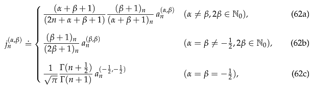
3. Fourier–Jacobi Coefficients

In this section, we use the integral representation (31) to obtain a formula for the computation of the Fourier–Jacobi coefficients of a function $f\left(x\right)$ from the Fourier coefficients of a suitable transform associated with a fractional integral of $f\left(x\right)$. Moreover, the symmetry properties of this latter transform allow us to define a class of renormalized Jacobi polynomials $J_n^{(\alpha ,\beta )}$, which are well defined also for negative values of the index n.

Let $f\left(x\right)$ be an integrable function that we wish to describe in terms of Jacobi polynomials, i.e.,

$$f\left(x\right)\sim \sum _{n=0}^{\infty }{a}_n^{(\alpha ,\beta )}{P}_n^{(\alpha ,\beta )}\left(x\right)(x\in [-1,1]),$$

(37)

where the coefficients are

$$\begin{array}{cc}\hfill a_n^{(\alpha ,\beta )}& ={\displaystyle \frac{1}{h_n^{(\alpha ,\beta )}}}{\int }_{-1}^{1}f\left(x\right)P_n^{(\alpha ,\beta )}\left(x\right){(1-x)}^{\alpha }{(1+x)}^{\beta }\mathrm{d}x\hfill \\ & ={\displaystyle \frac{1}{h_n^{(\alpha ,\beta )}}}{\int }_0^{\pi }f(cosu)P_n^{(\alpha ,\beta )}(cosu){(1-cosu)}^{\alpha }{(1+cosu)}^{\beta }sinu\mathrm{d}u,\hfill \end{array}$$

(38)

with $h_n^{(\alpha ,\beta )}$ being given in (8). In view of the equiconvergence theorem for the Jacobi series ([27], Theorem 9.1.2), the assumptions on $f\left(x\right)$ that guarantee the uniform convergence of expansion (37) in the compact intervals contained in $(-1,1)$ are analogous to the conditions necessary to have the uniform convergence of a Fourier series. Uniform convergence in $x\in [-1,1]$ requires instead stricter conditions on $f\left(x\right)$ (see, e.g., [31]). For example, if $f\left(x\right)$ is analytic on the closed segment $x\in [-1,1]$, then the spectral convergence of (37) is attained in the complex x-plane within the Bernstein ellipse with foci at $x=\pm 1$ ([27], Theorem 9.1.1). We now define the renormalized Fourier–Jacobi coefficients ${\overline{a}}_n^{(\alpha ,\beta )}$ as follows:

$${\overline{a}}_n^{(\alpha ,\beta )}\doteq {\displaystyle \frac{2\sqrt{\pi }\mathsf{\Gamma }(n+\beta +1)\mathsf{\Gamma }(\alpha -\beta )}{(2n+\alpha +\beta +1)\mathsf{\Gamma }(n+\alpha +\beta +1)}}{a}_n^{(\alpha ,\beta )}.$$

(39)

We can prove the following theorem.

Theorem 2. 

For $\alpha >\beta >-{\displaystyle \frac{1}{2}}$ and $n⩾0$, the coefficients ${\overline{a}}_n^{(\alpha ,\beta )}$ can be represented as follows:

$${\overline{a}}_n^{(\alpha ,\beta )}={\int }_0^1{(1-R)}^{\alpha -\beta -1}{R}^{n+2\beta +1}{\phi }_n^{(\beta +{\displaystyle \frac{1}{2}})}\left(R\right)\mathrm{d}R,$$

(40)

where, for every $R\in [0,1]$, ${\phi }_n^{\left(\beta \right)}\left(R\right)$ ($n⩾0$) denote the Fourier coefficients of the $2\pi$-periodic Abel-type transform ${\widehat{F}}_R^{\left(\beta \right)}\left(t\right)$ of $F_R\left(x\right)\doteq f(2R(1-x)-1)$, i.e.,

$${\phi }_n^{\left(\beta \right)}\left(R\right)={\int }_{-\pi }^{\pi }{\widehat{F}}_R^{\left(\beta \right)}\left(t\right)e^{\mathrm{i}nt}\mathrm{d}t(n⩾0;\beta >0),$$

(41)

and

$${\widehat{F}}_R^{\left(\beta \right)}\left(t\right)=e^{\mathrm{i}\beta (t-\pi ϵ(t\left)\right)}{I}^{\left(\beta \right)}\left[F_R\right]\left({sin}^2(t/2)\right)(\beta >0),$$

(42)

with $I^{\left(\beta \right)}\left[F_R\right](·)$ denoting the Riemann–Liouville fractional integral of $F_R\left(x\right)$ and $ϵ\left(t\right)$ being the sign function.

Proof. 

In Formula (38), we apply representation (31) of the Jacobi polynomials and obtain

$$\begin{array}{cc}\hfill a_n^{(\alpha ,\beta )}& ={\gamma }_n^{(\alpha ,\beta )}{e}^{-\mathrm{i}(\beta +{\displaystyle \frac{1}{2}})\pi }{\int }_0^{\pi }\mathrm{d}uf(cosu)sinu{\int }_{{\displaystyle \frac{1+cosu}{2}}}^1\mathrm{d}R{(1-R)}^{\alpha -\beta -1}{R}^{n+2\beta }\hfill \\ & \times {\int }_{v_u\left(R\right)}^{2\pi -v_u\left(R\right)}{e}^{\mathrm{i}(n+\beta +{\displaystyle \frac{1}{2}})t}{\left(cos{v}_u\left(R\right)-cost\right)}^{\beta -{\displaystyle \frac{1}{2}}}\mathrm{d}t,\hfill \end{array}$$

(43)

where ${\gamma }_n^{(\alpha ,\beta )}={\kappa }_n^{(\alpha ,\beta )}/h_n^{(\alpha ,\beta )}$ (see (8) and (30)) and $cos{v}_u\left(R\right)=(1+cosu-R)/R$. Now, we swap in (43) the first two integrals:

$$\begin{array}{cc}\hfill a_n^{(\alpha ,\beta )}& ={\gamma }_n^{(\alpha ,\beta )}{\int }_0^1\mathrm{d}R{(1-R)}^{\alpha -\beta -1}{R}^{n+2\beta }\hfill \\ & \times e^{-\mathrm{i}(\beta +{\displaystyle \frac{1}{2}})\pi }{\int }_{u_0\left(R\right)}^{\pi }\mathrm{d}uf(cosu)sinu{\int }_{v_u\left(R\right)}^{2\pi -v_u\left(R\right)}{e}^{\mathrm{i}(n+\beta +{\displaystyle \frac{1}{2}})t}{\left(cos{v}_u\left(R\right)-cost\right)}^{\beta -{\displaystyle \frac{1}{2}}}\mathrm{d}t,\hfill \end{array}$$

(44)

where $u_0\left(R\right)=arccos(2R-1)$. Our goal now is to manipulate the last two integrals in (44) to obtain a representation in terms of the Fourier coefficients of a proper Abel-type transform of $f\left(x\right)$. The integration domain in the $(u,t)$-plane is the curvilinear triangle whose sides are the curves $v_R\left(u\right)$, $2\pi -v_R\left(u\right)$ and the segment $u=u_0\left(R\right)$ (see Figure 2).

Then, swapping the last two integrals in (44), we have

$$\begin{array}{cc}& e^{-\mathrm{i}(\beta +{\displaystyle \frac{1}{2}})\pi }{\int }_{u_0\left(R\right)}^{\pi }\mathrm{d}uf(cosu)sinu{\int }_{v_R\left(u\right)}^{2\pi -v_R\left(u\right)}{e}^{\mathrm{i}(n+\beta +{\displaystyle \frac{1}{2}})t}{\left(cos{v}_R\left(u\right)-cost\right)}^{\beta -{\displaystyle \frac{1}{2}}}\mathrm{d}t\hfill \\ & =e^{-\mathrm{i}(\beta +{\displaystyle \frac{1}{2}})\pi }\left[{\int }_0^{\pi }\mathrm{d}t{e}^{\mathrm{i}(n+\beta +{\displaystyle \frac{1}{2}})t}{\int }_{u_0\left(R\right)}^{v_R^{-1}\left(t\right)}f(cosu){\left(cos{v}_R\left(u\right)-cost\right)}^{\beta -{\displaystyle \frac{1}{2}}}sinu\mathrm{d}u\right.\hfill \\ & +\left.{\int }_{\pi }^{2\pi }\mathrm{d}t{e}^{\mathrm{i}(n+\beta +{\displaystyle \frac{1}{2}})t}{\int }_{u_0\left(R\right)}^{2\pi -v_R^{-1}\left(t\right)}f(cosu){\left(cos{v}_R\left(u\right)-cost\right)}^{\beta -{\displaystyle \frac{1}{2}}}sinu\mathrm{d}u\right],\hfill \end{array}$$

(45)

where $v_R^{-1}\left(t\right)=arccos(Rcost+R-1)$. In the second term on the right-hand side of (45), we shift the integration variable $t\to t+2\pi$, which, since $v_R^{-1}(t+2\pi )=2\pi -v_R^{-1}\left(t\right)$, becomes

$$e^{\mathrm{i}(\beta +{\displaystyle \frac{1}{2}})2\pi }{\int }_{-\pi }^0\mathrm{d}t{e}^{\mathrm{i}(n+\beta +{\displaystyle \frac{1}{2}})t}{\int }_{u_0\left(R\right)}^{v_R^{-1}\left(t\right)}f(cosu){\left(cos{v}_R\left(u\right)-cost\right)}^{\beta -{\displaystyle \frac{1}{2}}}sinu\mathrm{d}u.$$

(46)

Finally, from (45) and (46), we have

$$\begin{array}{cc}& e^{-\mathrm{i}(\beta +{\displaystyle \frac{1}{2}})\pi }{\int }_{u_0\left(R\right)}^{\pi }\mathrm{d}uf(cosu)sinu{\int }_{v_R\left(u\right)}^{2\pi -v_R\left(u\right)}{e}^{\mathrm{i}(n+\beta +{\displaystyle \frac{1}{2}})t}{\left(cos{v}_R\left(u\right)-cost\right)}^{\beta -{\displaystyle \frac{1}{2}}}\mathrm{d}t\hfill \\ & ={\int }_{-\pi }^{\pi }{\mathcal{A}}_R^{(\beta +{\displaystyle \frac{1}{2}})}\left(t\right)e^{\mathrm{i}nt}\mathrm{d}t,\hfill \end{array}$$

(47)

where

$${\mathcal{A}}_R^{(\beta +{\displaystyle \frac{1}{2}})}\left(t\right)=e^{\mathrm{i}(\beta +{\displaystyle \frac{1}{2}})[t-\pi ϵ\left(t\right)]}{\int }_{u_0\left(R\right)}^{v_R^{-1}\left(t\right)}f(cosu){\left(cos{v}_R\left(u\right)-cost\right)}^{\beta -{\displaystyle \frac{1}{2}}}sinu\mathrm{d}u,$$

(48)

with $ϵ\left(t\right)$ denoting the sign function. We introduce in (48) the integration variable $x=1-{cos}^2(u/2)/R$, and we use $cos{v}_R\left(u\right)=(1+cosu-R)/R$ and $v_R^{-1}\left(t\right)=arccos(Rcost+R-1)$, so the Abel-type transform (48) can be written in the following form:

$$\begin{array}{cc}\hfill {\mathcal{A}}_R^{(\beta +{\displaystyle \frac{1}{2}})}\left(t\right)& =2^{\beta +{\displaystyle \frac{1}{2}}}R{e}^{\mathrm{i}(\beta +{\displaystyle \frac{1}{2}})[t-\pi ϵ\left(t\right)]}{\int }_0^{{sin}^2(t/2)}f(2R(1-x)-1){\left({sin}^2(t/2)-x\right)}^{\beta -{\displaystyle \frac{1}{2}}}\mathrm{d}x\hfill \\ & =2^{\beta +{\displaystyle \frac{1}{2}}}\mathsf{\Gamma }(\beta +\frac{1}{2})R{e}^{\mathrm{i}(\beta +{\displaystyle \frac{1}{2}})[t-\pi ϵ\left(t\right)]}{I}^{(\beta +{\displaystyle \frac{1}{2}})}\left[F_R\right]\left({sin}^2(t/2)\right),\hfill \end{array}$$

(49)

where $F_R\left(x\right)=f(2R(1-x)-1)$, and $I^{\left(\lambda \right)}\left[g\right]\left(x\right)$ denotes the Riemann–Liouville integral

$$I^{\left(\lambda \right)}\left[g\right]\left(y\right)={\displaystyle \frac{1}{\mathsf{\Gamma }\left(\lambda \right)}}{\int }_0^{y}g\left(x\right){(y-x)}^{\lambda -1}\mathrm{d}x(\mathrm{Re}\lambda >0),$$

(50)

which, for $\mathrm{Re}\lambda >0$, is well defined for a locally integrable function $g\left(x\right)$ and represents a bounded linear operator on $L^p(0,1)$ ($p⩾1$). It is worth recalling that $I^{\left(\lambda \right)}\left[g\right]\left(y\right)$ enjoys the properties

$${\displaystyle \frac{\mathrm{d}}{\mathrm{d}y}}{I}^{(\lambda +1)}\left[g\right]\left(y\right)=I^{\left(\lambda \right)}\left[g\right]\left(y\right),I^{\left(\lambda \right)}\left[I^{\left(\gamma \right)}\left[g\right]\right]\left(y\right)=I^{(\lambda +\gamma )}\left[g\right]\left(y\right),$$

(51)

and $I^{\left(\lambda \right)}\left[g\right]\left(y\right)$ is a Fourier multiplier: $\mathcal{L}\left(I^{\left(\lambda \right)}\left[g\right]\right)\left(s\right)=s^{-\lambda }\mathcal{L}\left[g\right]\left(s\right)$. Finally, from (44), (47) and (49), the statement of the theorem follows. □

Representation (40) and, in particular, Formula (42) for the Abel-type transform ${\widehat{F}}_R^{\left(\beta \right)}\left(t\right)$, which is given in terms of a Riemann–Liouville integral, make explicit and manifest the strict connection between Jacobi polynomials and fractional calculus. This already known fact appears, e.g., in Formula (35), which describes the Jacobi polynomials as a fractional integral involving the Gegenbauer polynomials. Another example in this sense is the Bateman fractional integral (36) for the hypergeometric series ${}_{2}F_1$, which can be easily reformulated for the Jacobi polynomials via Formula (6). Due to the non-local nature of the fractional derivatives, several attempts have been made to develop spectral methods for the solution of fractional differential equations and fractional variational problems. In this setting, it is therefore not surprising that Jacobi polynomials and the related associated functions, e.g., generalized Jacobi functions [32,33] and Jacobi poly-fractonomials [34], have shown attractive fractional calculus properties and remarkable capabilities in approximating functions, even with singular behaviors at the boundaries [32] (for applications of Jacobi polynomials to fractional calculus, see, e.g., [35,36,37,38,39,40] and the references therein). From this point of view, representation (40)–(42) of the Fourier–Jacobi coefficients appears to be particularly well suited to the construction of spectral schemes for the numerical solution of fractional calculus problems.

The representation of the Fourier–Jacobi coefficients given in Theorem 2 can be beneficial also from a computational viewpoint. Criticality in the computation of the coefficients $a_n^{(\alpha ,\beta )}$ emerges when the index n is very large and integral (38) becomes a highly oscillating integral. In this case, the quadrature of this integral becomes a difficult problem requiring the choice of exceedingly small subintervals. On the other hand, Theorem 2 shows that the burden of the oscillatory analysis is shifted to the Fourier integral (41), allowing us to take advantage of the computational efficiency and accuracy of the Fast Fourier Transform [41].

3.1. Extension of the Fourier–Jacobi Coefficients ${\overline{a}}_n^{(\alpha ,\beta )}$ to Negative Index n

For some values of the parameters $\alpha$ and $\beta$, the definition of Fourier–Jacobi coefficients can be extended to negative values of n. The most direct method to extend a given sequence ${\left\{p_n\right\}}_{n⩾0}$, indexed by nonnegative integers, to negative integers ${\left\{p_{-n}\right\}}_{n⩾1}$ is through recurrence relations among the elements $p_n$, if any. In fact, if ${\left\{p_n\right\}}_{n⩾0}$ satisfies a homogeneous linear recurrence relation, then it can be uniquely extended to all integers n by requiring the recurrence relation to hold for all $n\in \mathbb{Z}$. Hereafter, in order to extend the definition of Fourier–Jacobi coefficients to negative values of n, we adopt a different approach based on the symmetry emerging from representation (40). It is interesting to note that some works in the literature arbitrarily assume the values of the Fourier–Jacobi coefficients to be null for negative values of n. For example, in the analysis of the generalized Jacobi polynomials [42], the proof that different definitions of these polynomials do actually coincide and lead to equivalent generalized Jacobi polynomials is given under the assumption that $P_n^{(\alpha ,\beta )}\left(x\right)=0$ for $n<0$ and $\alpha ,\beta \in \mathbb{R}$ ([42], Remark 2.4, p. 78). Similarly, in Ref. [43], Lewanowicz proposes methods for the construction of recurrence relations for the Jacobi polynomials. Even in this case, these procedures assume $P_n^{(\alpha ,\beta )}\left(x\right)=0$ for $n<0$ if $\alpha \ne \beta$ of $\alpha =\beta$ but $2\alpha +1$ is not a nonnegative integral. As we will see in the following, these assumptions contradict the fact that, for certain sets of the parameters $\alpha$ and $\beta$, the values of the Fourier–Jacobi coefficients with $n<0$ are linear functionals of the coefficients with $n⩾0$ as a consequence of the symmetries of the Jacobi polynomials and, in general, are different from zero. Moreover, we will see how these symmetries lead naturally to the definition of a class of Jacobi polynomials with well-defined n-parity symmetry.

We start by noting that the Abel-type transform ${\widehat{F}}_R^{\left(\beta \right)}\left(t\right)$ in (42) enjoys the following symmetry:

$${\widehat{F}}_R^{\left(\beta \right)}\left(t\right)=e^{\mathrm{i}2\beta (t-\pi )}{\widehat{F}}_R^{\left(\beta \right)}(-t)(t\in \mathbb{R}),$$

(52)

which, for $2\beta \in {\mathbb{N}}_0$ (${\mathbb{N}}_0\doteq \mathbb{N}\cup \left\{0\right\}$), induces the following index symmetry for the Fourier coefficients ${\phi }_n^{\left(\beta \right)}\left(R\right)$:

$${\phi }_{-(n+2\beta )}^{\left(\beta \right)}\left(R\right)=e^{\mathrm{i}2\beta \pi }{\phi }_n^{\left(\beta \right)}\left(R\right)(n⩾0).$$

(53)

Relation (53) indicates a procedure to extend the definition of the normalized Fourier–Jacobi coefficients by symmetry to negative values of n by using those with a nonnegative index. Extending directly Formula (40) to negative values of n is not a feasible possibility in view of the divergence of the integrand in $R=0$ for $n⩽-2\beta -2$, unless ${\phi }_n^{\left(\beta \right)}\left(R\right)$ has in $R=0$ a zero of order higher than any power of R for $n⩽-2\beta -2$. In fact, ${\phi }_n^{\left(\beta \right)}\left(0\right)=0$ for $n⩽-2\beta -2$, but the order of the zero depends on the function $f\left(x\right)$. Nevertheless, we can select values of $\alpha$ and $\beta$ that lead to the proper definition of the Fourier–Jacobi coefficients for $n<0$ independently of $f\left(x\right)$.

For the sake of convenience, let us consider the normalized Fourier–Jacobi coefficients ${\overline{a}}_n^{(\alpha +{\displaystyle \frac{1}{2}},\beta -{\displaystyle \frac{1}{2}})}$, which, in view of (40), can be written as

$${\overline{a}}_n^{(\alpha +{\displaystyle \frac{1}{2}},\beta -{\displaystyle \frac{1}{2}})}={\int }_0^1{(1-R)}^{\alpha -\beta }{R}^{n+2\beta }{\phi }_n^{\left(\beta \right)}\left(R\right)\mathrm{d}R(n⩾0;\alpha +1>\beta >0).$$

(54)

Now, consider the normalized Fourier–Jacobi coefficient with negative index ${\overline{a}}_{-(n+2\beta )}^{(\alpha +{\displaystyle \frac{1}{2}},\beta -{\displaystyle \frac{1}{2}})}$ ($n⩾0$ and $2\beta \in \mathbb{N}$), which we aim to write in terms of well-defined normalized Fourier–Jacobi coefficients with a nonnegative index. From (54) and exploiting the symmetry relation (53), we formally have

$$\begin{array}{c}\hfill {\overline{a}}_{-(n+2\beta )}^{(\alpha +{\displaystyle \frac{1}{2}},\beta -{\displaystyle \frac{1}{2}})}=e^{\mathrm{i}2\beta \pi }{\int }_0^1{(1-R)}^{\alpha -\beta }{R}^{-2n-2\beta }{R}^{n+2\beta }{\phi }_n^{\left(\beta \right)}\left(R\right)\mathrm{d}R(n⩾0,2\beta \in \mathbb{N},\alpha >\beta -1),\end{array}$$

(55)

which has a structure similar to (54) but for the factor $R^{-2n-2\beta }$, which makes the integral divergent for $n⩾1$. This latter factor can be rewritten by making use of the binomial expansion

$$R^{-2n-2\beta }=\sum _{\ell =0}^{\infty }\left({\displaystyle \genfrac{}{}{0pt}{}{\ell +2n+2\beta -1}{\ell }}\right){(1-R)}^{\ell }\left(\right|R|<1).$$

(56)

After plugging (56) into the right-hand side of (55), swapping the series and integral and re-indexing, we obtain formally

$${\overline{a}}_{-(n+2\beta +1)}^{(\alpha ,\beta )}=e^{\mathrm{i}(2\beta +1)\pi }\sum _{\ell =0}^{\infty }\left({\displaystyle \genfrac{}{}{0pt}{}{\ell +2n+2\beta }{\ell }}\right){\overline{a}}_n^{(\alpha +\ell ,\beta )}(n⩾0,2\beta \in {\mathbb{N}}_0).$$

(57)

Formula (57) can be taken as the definition of the normalized Fourier–Jacobi coefficients with a negative index, provided that the series on the right-hand side converges. In this case, its validity can thus be extended by continuity to any value of $\alpha >-1$ and $2\beta \in \{-1\}\cup {\mathbb{N}}_0$.

Convergence issues in (57) are related to the divergence of integral (40) for $n⩽-2\beta -2$, as discussed previously. The series in (57) is summed over the values of the first parameter, i.e., $\alpha +\ell$, and therefore the convergence analysis requires uniform asymptotic estimates of ${\overline{a}}_n^{(\alpha ,\beta )}$ for $\alpha \to \infty$, which is a problem that is much less studied than the analogous one investigating asymptotics for $n\to \infty$. For instance, assuming that $f\left(x\right)$ is analytic in the Bernstein ellipse with foci in $x=\pm 1$ and the sum of the semi-axes $\rho >1$, we can make use of the uniform bound given by Zhao et al. [44] (Theorem 2.5), which yields, for $\alpha ,\beta >-1$, the estimate ${\overline{a}}_n^{(\alpha +\ell ,\beta )}=\mathcal{O}\left({\ell }^{-n-2\beta -2}\right)$ for $\ell \to \infty$. Hence, we have $\left({\displaystyle \genfrac{}{}{0pt}{}{\ell +2n+2\beta }{\ell }}\right){\overline{a}}_n^{(\alpha +\ell ,\beta )}=\mathcal{O}\left({\ell }^{n-2}\right)$ for $\ell \to \infty$, guaranteeing the convergence of (57) only for $n=0$. Nevertheless, as we will see later, representation (57) provides the Fourier–Jacobi coefficients with a negative index in important particular cases, which correspond to selected sets of values of $\alpha$ and $\beta$.

Remark 1. 

The reverse formula of (57), which gives the coefficients with a nonnegative index in terms of the coefficients with a negative index, can be obtained similarly. In fact, plugging the symmetry relation (53) into (54) yields

$$\begin{array}{cc}\hfill {\overline{a}}_n^{(\alpha +{\displaystyle \frac{1}{2}},\beta -{\displaystyle \frac{1}{2}})}=e^{-\mathrm{i}2\beta \pi }{\int }_0^1{(1-R)}^{\alpha -\beta }{R}^{2n+2\beta }& \left[R^{-(n+2\beta )+2\beta }{\phi }_{-(n+2\beta )}^{\left(\beta \right)}\left(R\right)\right]\mathrm{d}R\hfill \\ & (n⩾0,2\beta \in \mathbb{N},\alpha >\beta -1).\hfill \end{array}$$

(58)

Again, if $2\beta \in \mathbb{N}$, the factor $R^{2n+2\beta }$ can be expressed in terms of powers of $(1-R)$ by using the binomial expansion

$$R^m=\sum _{j=0}^m{(-1)}^j\left({\displaystyle \genfrac{}{}{0pt}{}{m}{j}}\right){(1-R)}^j(0⩽R<1),$$

(59)

with m being a finite nonnegative integer. Hence, from (58), we have formally

$$\begin{array}{cc}\hfill {\overline{a}}_n^{(\alpha +{\displaystyle \frac{1}{2}},\beta -{\displaystyle \frac{1}{2}})}& =e^{-\mathrm{i}2\beta \pi }\sum _{j=0}^{2n+2\beta }{(-1)}^j\left({\displaystyle \genfrac{}{}{0pt}{}{2n+2\beta }{j}}\right){\int }_0^1{(1-R)}^{(\alpha +j)-\beta }\left[R^{-n}{\phi }_{-(n+2\beta )}^{\left(\beta \right)}\left(R\right)\right]\mathrm{d}R,\hfill \end{array}$$

(60)

which, using (54) (and after shifting the indexes α and β), gives the following relation:

$${\overline{a}}_n^{(\alpha ,\beta )}=e^{-\mathrm{i}(2\beta +1)\pi }\sum _{j=0}^{2n+2\beta +1}{(-1)}^j\left({\displaystyle \genfrac{}{}{0pt}{}{2n+2\beta +1}{j}}\right){\overline{a}}_{-(n+2\beta +1)}^{(\alpha +j,\beta )}(n⩾0,2\beta \in {\mathbb{N}}_0).$$

(61)

There are many possible ways to normalize the Jacobi polynomials, and each one may have advantages and disadvantages. Jacobi polynomials, as defined through (4), are orthogonal on $[-1,1]$ with respect to $w^{(\alpha ,\beta )}\left(x\right)$ but, when divided by ${\left(h_n^{(\alpha ,\beta )}\right)}^{{\displaystyle \frac{1}{2}}}$, lead to a system of orthonormal polynomials, which yields advantages in the analysis and numerical computation of Fourier–Jacobi series. Nevertheless, definition (4) makes simple and transparent the x-parity (or $\alpha \leftrightarrow \beta$ swap) symmetry given in (11). Similarly, representation (40) of the normalized Fourier–Jacobi coefficients ${\overline{a}}_n^{(\alpha ,\beta )}$ makes clear the symmetry property of the Fourier coefficients ${\phi }_n^{\left(\beta \right)}\left(R\right)$ (see (53)). Hereafter, we will see how this symmetry can be exploited to define in a natural way suitably normalized Jacobi polynomials with n-parity symmetry.

Proposition 1. 

For $\alpha ,\beta >-1$, let the renormalized Fourier–Jacobi coefficients $j_n^{(\alpha ,\beta )}$ be defined as

where $a_n^{(\alpha ,\beta )}$ are the Fourier–Jacobi coefficients defined in (38). Then, for $2\beta \in \{-1\}\cup {\mathbb{N}}_0$, the corresponding Fourier–Jacobi coefficients with a negative index are given by

Proof. 

By using definition (40) of the normalized coefficients ${\overline{a}}_n^{(\alpha ,\beta )}$, let us rewrite Formula (57) in terms of the standard Fourier–Jacobi coefficients $a_n^{(\alpha ,\beta )}$ ($\alpha ,\beta >-1$). We have formally

$$\begin{array}{cc}& e^{-\mathrm{i}(2\beta +1)\pi }{\displaystyle \frac{\mathsf{\Gamma }(-n-\beta )}{(\alpha -2n-3\beta -1)\mathsf{\Gamma }(\alpha -\beta -n)}}{a}_{-n-2\beta -1}^{(\alpha ,\beta )}\hfill \\ & =\sum _{\ell =0}^{\infty }\left({\displaystyle \genfrac{}{}{0pt}{}{\ell +2n+2\beta }{\ell }}\right){\displaystyle \frac{\mathsf{\Gamma }(\alpha -\beta +\ell )}{\mathsf{\Gamma }(\alpha -\beta )}}{\displaystyle \frac{\mathsf{\Gamma }(n+\beta +1)}{(2n+\alpha +\beta +\ell +1)\mathsf{\Gamma }(n+\alpha +\beta +\ell +1)}}{a}_n^{(\alpha +\ell ,\beta )}.\hfill \end{array}$$

(64)

Formula (64) suggests that we define the class of Jacobi polynomials that admit the definition by symmetry of the corresponding Fourier–Jacobi coefficients with negative index n as a linear combination of Fourier–Jacobi coefficients with nonnegative n. First, we observe that Formula (64) simplifies if $\alpha =\beta \ne -{\displaystyle \frac{1}{2}}$ and $\alpha =\beta =-{\displaystyle \frac{1}{2}}$, which in these cases becomes

$$\begin{array}{cc}\hfill {\displaystyle \frac{\mathsf{\Gamma }(-n-\beta )}{\mathsf{\Gamma }(-n)}}{a}_{-n-2\beta -1}^{(\beta ,\beta )}& =e^{\mathrm{i}2\beta \pi }{\displaystyle \frac{\mathsf{\Gamma }(n+\beta +1)}{\mathsf{\Gamma }(n+2\beta +1)}}{a}_n^{(\beta ,\beta )}(\alpha =\beta \ne -\frac{1}{2}),\hfill \end{array}$$

(65)

$$\begin{array}{cc}\hfill {\displaystyle \frac{\mathsf{\Gamma }(-n+\frac{1}{2})}{\mathsf{\Gamma }(-n+1)}}{a}_{-n}^{(-{\displaystyle \frac{1}{2}},-{\displaystyle \frac{1}{2}})}& ={\displaystyle \frac{\mathsf{\Gamma }(n+\frac{1}{2})}{\mathsf{\Gamma }(n+1)}}{a}_n^{(-{\displaystyle \frac{1}{2}},-{\displaystyle \frac{1}{2}})}(\alpha =\beta =-\frac{1}{2}).\hfill \end{array}$$

(66)

We are then led to define the following Jacobi-type coefficients (associated with an integrable function $f\left(x\right)$):

$$j_n^{(\alpha ,\beta )}\doteq {\rho }^{(\alpha ,\beta )}{q}_n^{(\alpha ,\beta )}{a}_n^{(\alpha ,\beta )},$$

(67)

where (see (64)–(66))

$$q_n^{(\alpha ,\beta )}=\left\{\begin{array}{cc}{\displaystyle \phantom{(}\frac{\mathsf{\Gamma }(n+\beta +1)}{(2n+\alpha +\beta +1)\mathsf{\Gamma }(n+\alpha +\beta +1)}}\hfill & \mathrm{for}\alpha \ne \beta ,\hfill \\ {\displaystyle \phantom{(}\frac{\mathsf{\Gamma }(n+\beta +1)}{\mathsf{\Gamma }(n+2\beta +1)}}\hfill & \mathrm{for}\alpha =\beta \ne \frac{1}{2},\hfill \\ {\displaystyle \phantom{(}\frac{\mathsf{\Gamma }(n+\frac{1}{2})}{\mathsf{\Gamma }(n+1)}}\hfill & \mathrm{for}\alpha =\beta =-\frac{1}{2},\hfill \end{array}\right.$$

(68)

and ${\rho }^{(\alpha ,\beta )}$ is a constant that is independent of n, still to be defined. The coefficients $j_n^{(\alpha ,\beta )}$ are supposed to be spectral projections of the function $f\left(x\right)$ over the renormalized Jacobi polynomials $J_n^{(\alpha ,\beta )}\left(x\right)\doteq C_n^{(\alpha ,\beta )}{P}_n^{(\alpha ,\beta )}\left(x\right)$, i.e.,

$$j_n^{(\alpha ,\beta )}={\displaystyle \frac{1}{g_n^{(\alpha ,\beta )}}}{\int }_{-1}^{1}f\left(x\right)J_n^{(\alpha ,\beta )}\left(x\right){(1-x)}^{\alpha }{(1+x)}^{\beta }\mathrm{d}x={\displaystyle \frac{C_n^{(\alpha ,\beta )}{h}_n^{(\alpha ,\beta )}}{g_n^{(\alpha ,\beta )}}}{a}_n^{(\alpha ,\beta )},$$

(69)

with $g_n^{(\alpha ,\beta )}$ being the normalization constant

$$g_n^{(\alpha ,\beta )}={\int }_{-1}^1{\left(J_n^{(\alpha ,\beta )}\left(x\right)\right)}^2{(1-x)}^{\alpha }{(1+x)}^{\beta }\mathrm{d}x={\left(C_n^{(\alpha ,\beta )}\right)}^2{h}_n^{(\alpha ,\beta )},$$

(70)

where $h_n^{(\alpha ,\beta )}$ is defined in (8). Therefore, from (69) and (70), we have $j_n^{(\alpha ,\beta )}=a_n^{(\alpha ,\beta )}/C_n^{(\alpha ,\beta )}$, and, consequently, from (67), $C_n^{(\alpha ,\beta )}={\left({\rho }^{(\alpha ,\beta )}{q}_n^{(\alpha ,\beta )}\right)}^{-1}$. Now, we assume that, for $n=0$, the polynomials $J_0^{(\alpha ,\beta )}\left(x\right)$ and $P_0^{(\alpha ,\beta )}\left(x\right)$, which, in this case, are constant, do coincide, i.e., we assume $C_0^{(\alpha ,\beta )}=1$. It then follows that ${\rho }^{(\alpha ,\beta )}=1/q_0^{(\alpha ,\beta )}$ and therefore $C_n^{(\alpha ,\beta )}=q_0^{(\alpha ,\beta )}/q_n^{(\alpha ,\beta )}$. Hence, the renormalized Fourier–Jacobi coefficients are defined by (see (67))

$$j_n^{(\alpha ,\beta )}\doteq {\displaystyle \frac{q_n^{(\alpha ,\beta )}}{q_0^{(\alpha ,\beta )}}}{a}_n^{(\alpha ,\beta )},$$

(71)

whose explicit expression is given by Formula (62). Correspondingly, the renormalized Jacobi polynomials are defined by $J_n^{(\alpha ,\beta )}\left(x\right)\doteq (q_0^{(\alpha ,\beta )}/q_n^{(\alpha ,\beta )})P_n^{(\alpha ,\beta )}\left(x\right)$. Finally, plugging definition (62) of $j_n^{(\alpha ,\beta )}$ into (64), we obtain Formula (63) for the coefficients $j_{-n-2\beta -1}^{(\alpha ,\beta )}$ with a negative index. □

The case $\alpha =\beta =-{\displaystyle \frac{1}{2}}$, given in (62c), corresponds to the coefficients associated with the Chebyshev polynomials of the first kind, $T_n\left(x\right)\equiv J_n^{(-{\displaystyle \frac{1}{2}},-{\displaystyle \frac{1}{2}})}\left(x\right)=\sqrt{\pi }\mathsf{\Gamma }(n+1)/\mathsf{\Gamma }(n+{\displaystyle \frac{1}{2}})P_n^{(-{\displaystyle \frac{1}{2}},-{\displaystyle \frac{1}{2}})}\left(x\right)$ ([45], (10.11.5), p. 184), whose coefficients $t_n\equiv j_n^{(-{\displaystyle \frac{1}{2}},-{\displaystyle \frac{1}{2}})}$ satisfy the symmetry $t_{-n}=t_n$ for $n\in \mathbb{Z}$ (see (63c)). It is worth observing that the factor $\mathsf{\Gamma }(-n+{\displaystyle \frac{1}{2}})/\mathsf{\Gamma }(-n+1)$ is indeed what makes $t_{-n}$ finite and well defined, compensating for the divergence of $a_{-n}^{(-{\displaystyle \frac{1}{2}},-{\displaystyle \frac{1}{2}})}$ for $n⩾1$. The case $\alpha =\beta ={\displaystyle \frac{1}{2}}$ (see (62b)) represents the Chebyshev polynomials of the second kind ([45], (10.11.6), p. 184),

$$U_n\left(x\right)\equiv J_n^{({\displaystyle \frac{1}{2}},{\displaystyle \frac{1}{2}})}\left(x\right)={\displaystyle \frac{\sqrt{\pi }}{2}}{\displaystyle \frac{\mathsf{\Gamma }(n+2)}{\mathsf{\Gamma }(n+3/2)}}{P}_n^{({\displaystyle \frac{1}{2}},{\displaystyle \frac{1}{2}})}\left(x\right),$$

(72)

whose coefficients $u_n\equiv j_n^{({\displaystyle \frac{1}{2}},{\displaystyle \frac{1}{2}})}$ satisfy the symmetry relation $u_{-n-2}=-u_n$ (see (63b)). More generally, adopting the standard notation, when $\alpha =\beta =\lambda -{\displaystyle \frac{1}{2}}$ ($\lambda >0$), from (62b), we have the coefficients associated with the ultraspherical (Gegenbauer) polynomials ([45], (10.9.4), p. 174):

$$C_n^{\left(\lambda \right)}\left(x\right)\equiv J_n^{(\lambda -{\displaystyle \frac{1}{2}},\lambda -{\displaystyle \frac{1}{2}})}\left(x\right)={\displaystyle \frac{{\left(2\lambda \right)}_n}{{(\lambda +\frac{1}{2})}_n}}{P}_n^{(\lambda -{\displaystyle \frac{1}{2}},\lambda -{\displaystyle \frac{1}{2}})}\left(x\right),$$

(73)

whose coefficients $c_n^{\left(\lambda \right)}\equiv j_n^{(\lambda -{\displaystyle \frac{1}{2}},\lambda -{\displaystyle \frac{1}{2}})}$ enjoy the symmetry relation $c_{-n-2\lambda }^{\left(\lambda \right)}=-e^{\mathrm{i}2\lambda \pi }{c}_n^{\left(\lambda \right)}$ when $2\lambda \in \mathbb{N}$.

Evidently, the series in (63a) is affected by the convergence issues discussed earlier for the series in (64). Nevertheless, from (63a), we can select a subclass of Jacobi polynomials that are well defined even with negative values of n. Let $\alpha -\beta =-m$, $m\in {\mathbb{N}}_0$. The sum on the right-hand side of (63a) terminates since ${lim}_{(\alpha -\beta )\to -m}{(\alpha -\beta )}_{\ell }={(-1)}^{\ell }m!/(m-\ell )!$ for $\ell ⩽m$ and zero for $\ell >m$. Formula (63a) thus becomes

$$\begin{array}{c}\hfill j_{-n-2\beta -1}^{(\beta -m,\beta )}=m!e^{\mathrm{i}(2\beta +1)\pi }\sum _{\ell =0}^m\left({\displaystyle \genfrac{}{}{0pt}{}{\ell +2n+2\beta }{\ell }}\right){\displaystyle \frac{{(-1)}^{\ell }}{(m-\ell )!{(2\beta -m+2)}_{\ell }}}{j}_n^{(\beta -m+\ell ,\beta )}.\end{array}$$

(74)

As an example, let $\beta ={\displaystyle \frac{1}{2}}$ and $m=1$ (i.e., $\alpha =-{\displaystyle \frac{1}{2}}$). Formula (74) yields the Chebyshev coefficients of the third kind [46],

$$v_n\equiv j_n^{(-{\displaystyle \frac{1}{2}},{\displaystyle \frac{1}{2}})}={\displaystyle \frac{1}{\sqrt{\pi }}}{\displaystyle \frac{\mathsf{\Gamma }(n+\frac{1}{2})}{\mathsf{\Gamma }(n+1)}}{a}_n^{(-{\displaystyle \frac{1}{2}},{\displaystyle \frac{1}{2}})},$$

(75)

and, correspondingly, the symmetry relation (74) reads

$$j_{-n-2}^{(-{\displaystyle \frac{1}{2}},{\displaystyle \frac{1}{2}})}=\sum _{\ell =0}^1\left({\displaystyle \genfrac{}{}{0pt}{}{\ell +2n+1}{\ell }}\right){\displaystyle \frac{{(-1)}^{\ell }}{(1-\ell )!\mathsf{\Gamma }(\ell +2)}}{j}_n^{(-{\displaystyle \frac{1}{2}}+\ell ,{\displaystyle \frac{1}{2}})}=j_n^{(-{\displaystyle \frac{1}{2}},{\displaystyle \frac{1}{2}})}-(n+1)j_n^{({\displaystyle \frac{1}{2}},{\displaystyle \frac{1}{2}})}.$$

(76)

Now, making use of the recurrence relation (A9) for the polynomials $j_n^{(-{\displaystyle \frac{1}{2}},{\displaystyle \frac{1}{2}})}$ given in Appendix A, $j_n^{(-{\displaystyle \frac{1}{2}},{\displaystyle \frac{1}{2}})}=j_{n-1}^{(-{\displaystyle \frac{1}{2}},{\displaystyle \frac{1}{2}})}-n{j}_{n-1}^{({\displaystyle \frac{1}{2}},{\displaystyle \frac{1}{2}})}$, we obtain the usual symmetry relation for the coefficients associated with the Chebyshev polynomials of the third kind: $v_{-n-1}=v_n$.

3.2. Relations Between Coefficients ${\overline{a}}_n^{(\alpha ,\beta )}$ with Different Parameters

In this subsection, we see how the connections between coefficients ${\overline{a}}_n^{(\alpha ,\beta )}$ (see (39)) with different parameters follow from the corresponding relations satisfied by the Fourier coefficients ${\phi }_n^{\left(\beta \right)}\left(R\right)$ through representation (40) of Theorem 2. Similarly, we also prove the relation between the coefficients ${\overline{a}}_n^{(\alpha ,\beta )}$ of the derivatives and anti-derivatives of a function and the coefficients of the function itself.

3.2.1. Recurrence Relations

For notational convenience, it is useful to denote $E^{\left(\lambda \right)}\left(t\right)\doteq e^{\mathrm{i}\lambda [t-\pi ϵ(t\left)\right]}$, ${\tilde{I}}^{\left(\lambda \right)}\left(t\right)\doteq I^{\left(\lambda \right)}\left[F_R\right]\left({sin}^2(t/2)\right)$, and hence we rewrite Formula (42) as ${\widehat{F}}_R^{\left(\lambda \right)}\left(t\right)=E^{\left(\lambda \right)}\left(t\right){\tilde{I}}^{\left(\lambda \right)}\left(t\right)$. We first prove the following lemma.

Lemma 1. 

For $n⩾0$, $\beta >0$, $0⩽R⩽1$, the Fourier coefficients ${\phi }_n^{\left(\beta \right)}\left(R\right)$ (see definition (41)) satisfy the following relation:

$${\phi }_n^{(\beta +1)}\left(R\right)={\xi }_n^{\left(\beta \right)}\left({\phi }_n^{\left(\beta \right)}\left(R\right)-{\phi }_{n+2}^{\left(\beta \right)}\left(R\right)\right),$$

(77)

where

$${\xi }_n^{\left(\beta \right)}={\displaystyle \frac{1}{4(n+\beta +1)}}.$$

(78)

Proof. 

The first step is to obtain a suitable relation between the Abel-type transforms ${\widehat{F}}_R^{\left(\beta \right)}\left(t\right)$ with different values of $\beta$ (see (42)). To this end, we compute the derivative of the Riemann–Liouville integral ${\tilde{I}}^{(1+\beta )}\left(t\right)$ in two different ways. Equating the two results will give us the sought formula for ${\widehat{F}}_R^{\left(\beta \right)}\left(t\right)$. Using definition (50) for ${\tilde{I}}^{(1+\beta )}\left(t\right)$ (${\partial }_t\equiv \partial /\partial t$), we have

$${\partial }_t{\tilde{I}}^{(1+\beta )}\left(t\right)=\frac{1}{2}sint{\partial }_t{I}^{(1+\beta )}\left[F_R\right]\left({sin}^2(t/2)\right)=\frac{1}{2}sint{\tilde{I}}^{\left(\beta \right)}\left(t\right),$$

(79)

with the last equality following from property (51) of the Riemann–Liouville integrals. Then, in view of (42) and recalling that $E^{(1+\beta )}\left(t\right)=E^{\left(1\right)}\left(t\right)E^{\left(\beta \right)}\left(t\right)$, we can write

$$E^{(1+\beta )}\left(t\right){\partial }_t{\tilde{I}}^{(1+\beta )}\left(t\right)=\frac{1}{2}sint{E}^{\left(1\right)}\left(t\right)E^{\left(\beta \right)}\left(t\right){\partial }_t{\tilde{I}}^{\left(\beta \right)}\left(t\right)=\frac{1}{2}sint{E}^{\left(1\right)}\left(t\right){\widehat{F}}_R^{\left(\beta \right)}\left(t\right).$$

(80)

On the other hand, we can also use Formula (42) for ${\tilde{I}}^{(1+\beta )}\left(t\right)$ and obtain

$$\begin{array}{c}\hfill E^{(1+\beta )}\left(t\right){\partial }_t{\tilde{I}}^{(1+\beta )}\left(t\right)=E^{(1+\beta )}\left(t\right){\partial }_t\left({\displaystyle \frac{{\widehat{F}}_R^{(1+\beta )}\left(t\right)}{E^{(1+\beta )}\left(t\right)}}\right)={\partial }_t{\widehat{F}}_R^{(1+\beta )}\left(t\right)-{\tilde{I}}^{(1+\beta )}\left(t\right){\partial }_t{E}^{(1+\beta )}\left(t\right).\end{array}$$

(81)

The comparison of (80) with (81) gives us the relation

$$\frac{1}{2}sint{E}^{\left(1\right)}\left(t\right){\widehat{F}}_R^{\left(\beta \right)}\left(t\right)={\partial }_t{\widehat{F}}_R^{(1+\beta )}\left(t\right)-{\tilde{I}}^{(1+\beta )}\left(t\right){\partial }_t{E}^{(1+\beta )}\left(t\right).$$

(82)

Since $E^{(1+\beta )}\left(t\right)$ contains the discontinuous function $ϵ\left(t\right)$, the derivative ${\partial }_t{E}^{(1+\beta )}\left(t\right)$ is undefined in $t=0$, but it can be computed as a Schwartz distributional derivative (weak derivative) [47]. In this sense, we recall that ${\partial }_tϵ\left(t\right)=2\delta \left(t\right)$, where $\delta (·)$ denotes the Dirac delta function. Hence, with this prescription, we have

$${\partial }_t{E}^{(1+\beta )}\left(t\right)=\mathrm{i}(1+\beta )E^{(1+\beta )}\left(t\right){\partial }_t(t-\pi ϵ\left(t\right))=\mathrm{i}(1+\beta )E^{(1+\beta )}\left(t\right)(1-2\pi \delta \left(t\right)).$$

(83)

Plugging (83) into (82) yields the following formula relating Abel-type transforms ${\widehat{F}}_R^{\left(\beta \right)}\left(t\right)$ with different orders $\beta$:

$$\frac{1}{2}sint{E}^{\left(1\right)}\left(t\right){\widehat{F}}_R^{\left(\beta \right)}\left(t\right)={\partial }_t{\widehat{F}}_R^{(1+\beta )}\left(t\right)-\mathrm{i}(1+\beta ){\widehat{F}}_R^{(1+\beta )}\left(t\right)(1-2\pi \delta \left(t\right)).$$

(84)

Now, the subsequent step towards obtaining the relation among Fourier coefficients ${\phi }_n^{\left(\beta \right)}\left(R\right)$ with different values of n and $\beta$ is through definition (41). Thus, in (84), we multiply both sides by $e^{\mathrm{i}nt}$ and integrate over $[-\pi ,\pi ]$:

$$\begin{array}{cc}& {\displaystyle \frac{1}{2}}{\int }_{-\pi }^{\pi }{E}^{\left(1\right)}\left(t\right){\widehat{F}}_R^{\left(\beta \right)}\left(t\right)sint{e}^{\mathrm{i}nt}\mathrm{d}t={\int }_{-\pi }^{\pi }{\partial }_t{\widehat{F}}_R^{(1+\beta )}\left(t\right)e^{\mathrm{i}nt}\mathrm{d}t\hfill \\ & -\mathrm{i}(1+\beta ){\int }_{-\pi }^{\pi }{\widehat{F}}_R^{(1+\beta )}\left(t\right)e^{\mathrm{i}nt}\mathrm{d}t+2\pi \mathrm{i}(1+\beta ){\int }_{-\pi }^{\pi }{\widehat{F}}_R^{(1+\beta )}\left(t\right)\delta \left(t\right)e^{\mathrm{i}nt}\mathrm{d}t.\hfill \end{array}$$

(85)

The rightmost integral on the right-hand side of (85), which contains the Dirac delta function, is null since ${\widehat{F}}_R^{(1+\beta )}\left(0\right)=0$ (see (50)). Moreover, by the periodicity of ${\widehat{F}}_R^{(1+\beta )}\left(t\right)$ and recalling the expression for the Fourier coefficient of the derivative of a function, we have

$${\int }_{-\pi }^{\pi }{\partial }_t{\widehat{F}}_R^{(1+\beta )}\left(t\right)e^{\mathrm{i}nt}\mathrm{d}t=-\mathrm{i}n{\int }_{-\pi }^{\pi }{\widehat{F}}_R^{(1+\beta )}\left(t\right)e^{\mathrm{i}nt}\mathrm{d}t=-\mathrm{i}n{\phi }_n^{(1+\beta )}\left(R\right).$$

(86)

It remains to compute the integral on the left-hand side of (85); we have

$$\begin{array}{cc}& 2\mathrm{i}{\int }_{-\pi }^{\pi }{E}^{\left(1\right)}\left(t\right){\widehat{F}}_R^{\left(\beta \right)}\left(t\right)sint{e}^{\mathrm{i}nt}\mathrm{d}t={\int }_{-\pi }^{\pi }(e^{\mathrm{i}t}-e^{-\mathrm{i}t})E^{\left(1\right)}\left(t\right){\widehat{F}}_R^{\left(\beta \right)}\left(t\right)e^{\mathrm{i}nt}\mathrm{d}t\hfill \\ & ={\int }_{-\pi }^{\pi }{e}^{\mathrm{i}(t-\pi ϵ(t\left)\right)}{\widehat{F}}_R^{\left(\beta \right)}\left(t\right)e^{\mathrm{i}(n+1)t}\mathrm{d}t-{\int }_{-\pi }^{\pi }{e}^{\mathrm{i}(t-\pi ϵ(t\left)\right)}{\widehat{F}}_R^{\left(\beta \right)}\left(t\right)e^{\mathrm{i}(n-1)t}\mathrm{d}t.\hfill \end{array}$$

(87)

Let us calculate the first integral on the right-hand side of (87), with the computation of the second integral being similar:

$$\begin{array}{cc}& {\int }_{-\pi }^{\pi }{e}^{\mathrm{i}(t-\pi ϵ(t\left)\right)}{\widehat{F}}_R^{\left(\beta \right)}\left(t\right)e^{\mathrm{i}(n+1)t}\mathrm{d}t\hfill \\ & ={\int }_{-\pi }^0{e}^{\mathrm{i}(t+\pi )}{\widehat{F}}_R^{\left(\beta \right)}\left(t\right)e^{\mathrm{i}(n+1)t}\mathrm{d}t+{\int }_0^{\pi }{e}^{\mathrm{i}(t-\pi )}{\widehat{F}}_R^{\left(\beta \right)}\left(t\right)e^{\mathrm{i}(n+1)t}\mathrm{d}t\hfill \\ & ={\int }_0^{\pi }{e}^{-\mathrm{i}(t-\pi )}{\widehat{F}}_R^{\left(\beta \right)}(-t)e^{-\mathrm{i}(n+1)t}\mathrm{d}t+{\int }_0^{\pi }{e}^{\mathrm{i}(t-\pi )}{\widehat{F}}_R^{\left(\beta \right)}\left(t\right)e^{\mathrm{i}(n+1)t}\mathrm{d}t\hfill \\ & =-{\int }_0^{\pi }{\widehat{F}}_R^{\left(\beta \right)}\left(t\right)\left[e^{-\mathrm{i}2\beta (t-\pi )}{e}^{-\mathrm{i}(n+2)t}+e^{\mathrm{i}(n+2)t}\right]\mathrm{d}t\hfill \\ & =-{\int }_0^{\pi }{\widehat{F}}_R^{\left(\beta \right)}\left(t\right)e^{-\mathrm{i}\beta (t-\pi )}\left[e^{-\mathrm{i}\left(\right(n+2)t+\beta (t-\pi \left)\right)}+e^{\mathrm{i}\left(\right(n+2)t+\beta (t-\pi \left)\right)}\right]\mathrm{d}t,\hfill \end{array}$$

(88)

where we use also the parity property of ${\widehat{F}}_R^{\left(\beta \right)}\left(t\right)$ in (52). In a very similar way, we have also

$${\int }_{-\pi }^{\pi }{e}^{\mathrm{i}(t-\pi ϵ(t\left)\right)}{\widehat{F}}_R^{\left(\beta \right)}\left(t\right)e^{\mathrm{i}(n-1)t}\mathrm{d}t=-{\int }_0^{\pi }{\widehat{F}}_R^{\left(\beta \right)}\left(t\right)e^{-\mathrm{i}\beta (t-\pi )}\left[e^{-\mathrm{i}(nt+\beta (t-\pi \left)\right)}+e^{\mathrm{i}(nt+\beta (t-\pi \left)\right)}\right]\mathrm{d}t.$$

(89)

Therefore, from (87), we obtain

$$\begin{array}{cc}& {\int }_{-\pi }^{\pi }{E}^{\left(1\right)}\left(t\right){\widehat{F}}_R^{\left(\beta \right)}\left(t\right)sint{e}^{\mathrm{i}nt}\mathrm{d}t=-{\displaystyle \frac{\mathrm{i}}{2}}{\int }_0^{\pi }{\widehat{F}}_R^{\left(\beta \right)}\left(t\right)e^{-\mathrm{i}\beta (t-\pi )}\hfill \\ & \times \left\{\left[e^{-\mathrm{i}(nt+\beta (t-\pi \left)\right)}+e^{\mathrm{i}(nt+\beta (t-\pi \left)\right)}\right]-\left[e^{-\mathrm{i}\left(\right(n+2)t+\beta (t-\pi \left)\right)}+e^{\mathrm{i}\left(\right(n+2)t+\beta (t-\pi \left)\right)}\right]\right\}\mathrm{d}t.\hfill \end{array}$$

(90)

From definition (41) and using (52), we see that ${\phi }_n^{\left(\beta \right)}\left(R\right)$ can be written also in the following alternative way:

$$\begin{array}{cc}\hfill {\phi }_n^{\left(\beta \right)}\left(R\right)& ={\int }_{-\pi }^{\pi }{\widehat{F}}_R^{\left(\beta \right)}\left(t\right)e^{\mathrm{i}nt}\mathrm{d}t={\int }_0^{\pi }\left[{\widehat{F}}_R^{\left(\beta \right)}(-t)e^{-\mathrm{i}nt}+{\widehat{F}}_R^{\left(\beta \right)}\left(t\right)e^{\mathrm{i}nt}\right]\mathrm{d}t\hfill \\ & ={\int }_0^{\pi }{\widehat{F}}_R^{\left(\beta \right)}\left(t\right)\left[e^{-\mathrm{i}2\beta (t-\pi )}{e}^{-\mathrm{i}nt}+e^{\mathrm{i}nt}\right]\mathrm{d}t\hfill \\ & ={\int }_0^{\pi }{\widehat{F}}_R^{\left(\beta \right)}\left(t\right)e^{-\mathrm{i}\beta (t-\pi )}\left[e^{-\mathrm{i}[nt+\beta (t-\pi \left)\right]}+e^{\mathrm{i}[nt+\beta (t-\pi \left)\right]}\right]\mathrm{d}t.\hfill \end{array}$$

(91)

Thus, comparing (90) and (91), we have

$${\int }_{-\pi }^{\pi }{E}^{\left(1\right)}\left(t\right){\widehat{F}}_R^{\left(\beta \right)}\left(t\right)sint{e}^{\mathrm{i}nt}\mathrm{d}t=-{\displaystyle \frac{\mathrm{i}}{2}}\left({\phi }_n^{\left(\beta \right)}\left(R\right)-{\phi }_{n+2}^{\left(\beta \right)}\left(R\right)\right).$$

(92)

Finally, from (85), (86) and (92), the recurrence Formula (77) follows. □

In the next proposition, we see how the relation among Fourier coefficients ${\phi }_n^{\left(\beta \right)}\left(R\right)$ induces the recurrence relation for the Fourier–Jacobi coefficients ${\overline{a}}_n^{(\alpha ,\beta )}$.

Proposition 2. 

For $\alpha >\beta >-{\displaystyle \frac{1}{2}}$, $n⩾0$, the renormalized Fourier–Jacobi coefficients ${\overline{a}}_n^{(\alpha ,\beta )}$ (see (39)) satisfy the following recurrence relation:

$${\overline{a}}_{n+2}^{(\alpha ,\beta )}={\overline{a}}_n^{(\alpha +2,\beta )}-2{\overline{a}}_n^{(\alpha +1,\beta )}+{\overline{a}}_n^{(\alpha ,\beta )}-2(2n+2\beta +3){\overline{a}}_n^{(\alpha +1,\beta +1)}.$$

(93)

Proof. 

Let us multiply both sides of Formula (77) by ${(1-R)}^{\alpha -\beta -1}{R}^{n+2\beta +2}$ and integrate over $R\in [0,1]$. We have

$$\begin{array}{cc}& {\int }_0^1{(1-R)}^{\alpha -(\beta +1)}{R}^{n+2(\beta +1)}{\phi }_n^{(1+\beta )}\left(R\right)\mathrm{d}R\hfill \\ & ={\xi }_n^{\left(\beta \right)}\left[{\int }_0^1{(1-R)}^{(\alpha -1)-\beta }{R}^{n+2\beta }{R}^2{\phi }_n^{\left(\beta \right)}\left(R\right)\mathrm{d}R-{\int }_0^1{(1-R)}^{(\alpha -1)-\beta }{R}^{(n+2)+2\beta }{\phi }_{n+2}^{\left(\beta \right)}\left(R\right)\mathrm{d}R\right],\hfill \end{array}$$

(94)

which, in view of (54), yields

$${\overline{a}}_n^{(\alpha +{\displaystyle \frac{1}{2}},\beta +{\displaystyle \frac{1}{2}})}+{\xi }_n^{\left(\beta \right)}{\overline{a}}_{n+2}^{(\alpha -{\displaystyle \frac{1}{2}},\beta -{\displaystyle \frac{1}{2}})}={\xi }_n^{\left(\beta \right)}{\int }_0^1{(1-R)}^{(\alpha -1)-\beta }{R}^{n+2\beta }{R}^2{\phi }_n^{\left(\beta \right)}\left(R\right)\mathrm{d}R.$$

(95)

Concerning the computation of the integral on the right-hand side of (95), we use Formula (59) to represent $R^2$ in terms of powers of $(1-R)$, which, in this case, reads $R^2={(1-R)}^2-2(1-R)+1$. From (95), we then have

$$\begin{array}{cc}& {\int }_0^1{(1-R)}^{(\alpha -1)-\beta }{R}^{n+2\beta }{R}^2{\phi }_n^{\left(\beta \right)}\left(R\right)\mathrm{d}R\hfill \\ & ={\int }_0^1{(1-R)}^{(\alpha +1)-\beta }{R}^{n+2\beta }{\phi }_n^{\left(\beta \right)}\left(R\right)\mathrm{d}R\hfill \\ & -2{\int }_0^1{(1-R)}^{\alpha -\beta }{R}^{n+2\beta }{\phi }_n^{\left(\beta \right)}\left(R\right)\mathrm{d}R+{\int }_0^1{(1-R)}^{(\alpha -1)-\beta }{R}^{n+2\beta }{\phi }_n^{\left(\beta \right)}\left(R\right)\mathrm{d}R\hfill \\ & ={\overline{a}}_n^{(\alpha +{\displaystyle \frac{3}{2}},\beta -{\displaystyle \frac{1}{2}})}-2{\overline{a}}_n^{(\alpha +{\displaystyle \frac{1}{2}},\beta -{\displaystyle \frac{1}{2}})}+{\overline{a}}_n^{(\alpha -{\displaystyle \frac{1}{2}},\beta -{\displaystyle \frac{1}{2}})}.\hfill \end{array}$$

(96)

Plugging (96) into (95), shifting indexes $\alpha \to \alpha +{\displaystyle \frac{1}{2}},\beta \to \beta +{\displaystyle \frac{1}{2}}$ and accounting for (78), we finally obtain the recurrence relation (93). □

Let us see now an alternative procedure to obtain recurrence relations from representation (40).

Proposition 3. 

For $\alpha >\beta >-{\displaystyle \frac{1}{2}}$, $n⩾0$, the renormalized Fourier–Jacobi coefficients ${\overline{a}}_n^{(\alpha ,\beta )}$ (see (39)) satisfy the following recurrence relation:

$${\overline{a}}_{n+1}^{(\alpha ,\beta )}=2(\alpha -\beta -1){\overline{a}}_n^{(\alpha ,\beta +1)}+{\overline{a}}_n^{(\alpha +1,\beta )}-{\overline{a}}_n^{(\alpha ,\beta )}.$$

(97)

Proof. 

Consider the integral

$${\mathfrak{I}}_n^{(\alpha ,\beta )}={\int }_0^1{(1-R)}^{\alpha -\beta }{R}^{n+2\beta }{\partial }_R{\phi }_n^{\left(\beta \right)}\left(R\right)\mathrm{d}R,$$

(98)

where ${\partial }_R\equiv \partial /\partial R$. This integral can be computed in two ways: the first is integration by parts and the second involves computing explicitly the term ${\partial }_R{\phi }_n^{\left(\beta \right)}\left(R\right)$. The equality of the two results will lead to a relation among the normalized Fourier–Jacobi coefficients. Integrating (98) by parts, we have

$$\begin{array}{cc}\hfill {\mathfrak{I}}_n^{(\alpha ,\beta )}& ={\int }_0^1\left[(\alpha -\beta ){(1-R)}^{(\alpha -1)-\beta }{R}^{n+2\beta }-(n+2\beta ){(1-R)}^{\alpha -\beta }{R}^{n+2\beta -1}\right]{\phi }_n^{\left(\beta \right)}\mathrm{d}R\hfill \\ & =(\alpha -\beta ){\overline{a}}_n^{(\alpha -{\displaystyle \frac{1}{2}},\beta -{\displaystyle \frac{1}{2}})}-(n+2\beta ){\mathcal{W}}_n^{(\alpha ,\beta )},\hfill \end{array}$$

(99)

where, for convenience, we have named

$${\mathcal{W}}_n^{(\alpha ,\beta )}={\int }_0^1{(1-R)}^{\alpha -\beta }{R}^{n+2\beta -1}{\phi }_n^{\left(\beta \right)}\left(R\right)\mathrm{d}R.$$

(100)

Consider now the term ${\partial }_R{\phi }_n^{\left(\beta \right)}\left(R\right)={\int }_{-\pi }^{\pi }{\partial }_R{\widehat{F}}_R^{\left(\beta \right)}\left(t\right)e^{\mathrm{i}nt}\mathrm{d}t$. From (42), integrating by parts (we denote $f^{\left(m\right)}\left(z\right)\equiv {\mathrm{d}}^{m}f\left(z\right)/\mathrm{d}{z}^m$), we have

$$\begin{array}{cc}\hfill {\partial }_R{\widehat{F}}_R^{\left(\beta \right)}\left(t\right)& =2{\displaystyle \frac{E^{\left(\beta \right)}\left(t\right)}{\mathsf{\Gamma }\left(\beta \right)}}{\int }_0^{{sin}^2(t/2)}{f}^{\left(1\right)}(2R(1-x)-1)(1-x){({sin}^2(t/2)-x)}^{\beta -1}\mathrm{d}x\hfill \\ & =2{\displaystyle \frac{E^{\left(\beta \right)}\left(t\right)}{\mathsf{\Gamma }\left(\beta \right)}}\left[{cos}^2(t/2){\int }_0^{{sin}^2(t/2)}{f}^{\left(1\right)}(2R(1-x)-1){({sin}^2(t/2)-x)}^{\beta -1}\mathrm{d}x\right.\hfill \\ & \left.+{\int }_0^{{sin}^2(t/2)}{f}^{\left(1\right)}(2R(1-x)-1){({sin}^2(t/2)-x)}^{\beta }\mathrm{d}x\right]\hfill \\ & ={\displaystyle \frac{E^{\left(\beta \right)}\left(t\right)}{R\mathsf{\Gamma }\left(\beta \right)}}\left[f(2R-1){\left({sin}^2(t/2)\right)}^{\beta -1}\right.\hfill \\ & -(\beta -1){cos}^2(t/2){\int }_0^{{sin}^2(t/2)}f(2R(1-x)-1){({sin}^2(t/2)-x)}^{\beta -2}\mathrm{d}x\hfill \\ & \left.-\beta {\int }_0^{{sin}^2(t/2)}f(2R(1-x)-1){({sin}^2(t/2)-x)}^{\beta -1}\mathrm{d}x\right]\hfill \\ & ={\displaystyle \frac{f(2R-1)}{R}}{\displaystyle \frac{E^{\left(\beta \right)}\left(t\right)}{\mathsf{\Gamma }\left(\beta \right)}}{\left({sin}^2(t/2)\right)}^{\beta -1}-{\displaystyle \frac{1}{R}}{cos}^2(t/2)E^{\left(1\right)}\left(t\right){\widehat{F}}_R^{(\beta -1)}\left(t\right)-{\displaystyle \frac{\beta }{R}}{\widehat{F}}_R^{\left(\beta \right)}\left(t\right).\hfill \end{array}$$

(101)

Now, plugging (101) into the formula for ${\partial }_R{\phi }_n^{\left(\beta \right)}\left(R\right)$, we remain with the following integral: ${\int }_{-\pi }^{\pi }{E}^{\left(\beta \right)}\left(t\right){\left({sin}^2(t/2)\right)}^{\beta -1}{e}^{\mathrm{i}nt}\mathrm{d}t$. Using the integral representation of $1/B(x,y)$, where $B(x,y)$ is the Euler beta function ([48], Formula 8.381.4, p. 909), it can be shown that this integral is proportional to $1/B(2\beta +n,-n)$ and therefore it is null for $n\in {\mathbb{N}}_0$. Then, we have

$${\partial }_R{\phi }_n^{\left(\beta \right)}\left(R\right)=-{\displaystyle \frac{1}{R}}{\int }_{-\pi }^{\pi }{E}^{\left(1\right)}\left(t\right)(1-{sin}^2(t/2)){\widehat{F}}_R^{(\beta -1)}\left(t\right)e^{\mathrm{i}nt}\mathrm{d}t-{\displaystyle \frac{\beta }{R}}{\phi }_n^{\left(\beta \right)}\left(R\right).$$

(102)

Since

$$\begin{array}{c}\hfill {\int }_{-\pi }^{\pi }{E}^{\left(1\right)}\left(t\right){\widehat{F}}_R^{(\beta -1)}\left(t\right)e^{\mathrm{i}nt}\mathrm{d}t={\int }_{-\pi }^{\pi }{e}^{-\mathrm{i}\pi ϵ\left(t\right)}{\widehat{F}}_R^{(\beta -1)}\left(t\right)e^{\mathrm{i}(n+1)t}\mathrm{d}t=-{\phi }_{n+1}^{(\beta -1)}\left(R\right),\end{array}$$

(103)

it is easy to see that the integral in (102) can be written as

$${\int }_{-\pi }^{\pi }{E}^{\left(1\right)}\left(t\right)(1-{sin}^2(t/2)){\widehat{F}}_R^{(\beta -1)}\left(t\right)e^{\mathrm{i}nt}\mathrm{d}t=-{\displaystyle \frac{1}{2}}{\phi }_{n+1}^{(\beta -1)}\left(R\right)-{\displaystyle \frac{1}{4}}{\phi }_{n+2}^{(\beta -1)}\left(R\right)-{\displaystyle \frac{1}{4}}{\phi }_n^{(\beta -1)}\left(R\right).$$

(104)

Finally, making use of (77), Formula (102) becomes

$${\partial }_R{\phi }_n^{\left(\beta \right)}\left(R\right)={\displaystyle \frac{1}{2R}}\left({\phi }_{n+1}^{(\beta -1)}\left(R\right)+{\phi }_n^{(\beta -1)}\left(R\right)-2(n+2\beta ){\phi }_n^{\left(\beta \right)}\left(R\right)\right).$$

(105)

If we multiply both sides of (105) by ${(1-R)}^{\alpha -\beta }{R}^{n+2\beta }$ and integrate on $R\in (0,1)$, we obtain an expression for ${\mathfrak{I}}^{(\alpha ,\beta )}$ that, after manipulations, reads

$${\mathfrak{I}}^{(\alpha ,\beta )}={\displaystyle \frac{1}{2}}\left({\overline{a}}_{n+1}^{(\alpha -{\displaystyle \frac{1}{2}},\beta -{\displaystyle \frac{3}{2}})}+{\overline{a}}_n^{(\alpha -{\displaystyle \frac{1}{2}},\beta -{\displaystyle \frac{3}{2}})}-{\overline{a}}_n^{(\alpha +{\displaystyle \frac{1}{2}},\beta -{\displaystyle \frac{3}{2}})}\right)-(n+2\beta ){\mathcal{W}}_n^{(\alpha ,\beta )},$$

(106)

where ${\mathcal{W}}_n^{(\alpha ,\beta )}$ is given in (100). Finally, equating Formulae (99) and (106) and shifting the parameters $\alpha$ and $\beta$, we obtain the recurrence relation (97). □

For the sake of completeness, in Appendix A, we summarize some recurrence relations for the coefficients ${\overline{a}}_n^{(\alpha ,\beta )}$, which follow from (93), (97), and for the coefficients $j_n^{(\alpha ,\beta )}$, which follow from definition (62).

3.2.2. Fourier–Jacobi Coefficients of Derivatives and Anti-Derivatives

Our purpose here is to give the relation between the normalized Fourier–Jacobi coefficients of the function $f\left(x\right)$ and those of its derivatives $f^{\left(k\right)}\left(x\right)$ ($k=0,1,2,\dots$, $f^{\left(0\right)}\equiv f$). Let us consider the case of the first derivative, with the successive ones following readily by induction. For convenience, we update the notation and denote by $a_n^{(\alpha ,\beta )}\left[f^{\left(k\right)}\right]$ the Fourier–Jacobi coefficients of the kth derivative of $f\left(x\right)$ (see (38)). An analogous extension emerges for the normalized coefficients ${\overline{a}}_n^{(\alpha ,\beta )}\left[f^{\left(k\right)}\right]$ (see (40)) and the functions ${\phi }_n^{\left(\lambda \right)}\left[f^{\left(k\right)}\right]$ (see (41)) and ${\widehat{F}}_R^{\left(\lambda \right)}\left[f^{\left(k\right)}\right]$ (see (42)).

Proposition 4. 

The Fourier–Jacobi coefficients ${\overline{a}}_n^{(\alpha ,\beta )}\left[f^{\left(k\right)}\right]$ of the kth derivative (if $k>0$) and of the kth anti-derivative (if $k<0$) of $f\left(x\right)$ can be written as follows:

$${\overline{a}}_n^{(\alpha ,\beta )}\left[f^{\left(k\right)}\right]=2^{-k}{\overline{a}}_{n+k}^{(\alpha -k,\beta -k)}\left[f\right](k\in \mathbb{Z};\alpha ,\beta >max\{-1,k-1\};n⩾max\{0,-k\}),$$

(107)

where, for integral $k⩾0$, $f^{\left(k\right)}\left(x\right)={\mathrm{d}}^{k}f/\mathrm{d}{x}^k$, while, for integral $k<0$, $f^{\left(k\right)}\left(x\right)$ denotes the kth anti-derivative $f^{\left(k\right)}\left(x\right)={\int }^x{\int }^{x_1}{\int }^{x_{k-1}}f\left(x_k\right)\mathrm{d}{x}_k\cdots \mathrm{d}{x}_2\mathrm{d}{x}_1$.

Proof. 

Let us consider ${\widehat{F}}_R^{\left(\beta \right)}\left[f^{\left(1\right)}\right]\left(t\right)$ (see (42)); integrating by parts, we have

$$\begin{array}{cc}\hfill {\widehat{F}}_R^{\left(\beta \right)}\left[f^{\left(1\right)}\right]\left(t\right)& ={\displaystyle \frac{E^{\left(\beta \right)}\left(t\right)}{\mathsf{\Gamma }\left(\beta \right)}}{\int }_0^{{sin}^2(t/2)}{f}^{\left(1\right)}(2R(1-x)-1){({sin}^2(t/2)-x)}^{\beta -1}\mathrm{d}x\hfill \\ & ={\displaystyle \frac{E^{\left(\beta \right)}\left(t\right)}{2R\mathsf{\Gamma }\left(\beta \right)}}\left[f(2R-1){\left({sin}^2(t/2)\right)}^{\beta -1}\right.\hfill \\ & \left.-(\beta -1){\int }_0^{{sin}^2(t/2)}f(2R(1-x)-1){({sin}^2(t/2)-x)}^{\beta -2}\mathrm{d}x\right]\hfill \\ & ={\displaystyle \frac{f(2R-1)}{2R}}{\displaystyle \frac{E^{\left(\beta \right)}\left(t\right)}{\mathsf{\Gamma }\left(\beta \right)}}{\left({sin}^2(t/2)\right)}^{\beta -1}-{\displaystyle \frac{1}{2R}}{E}^{\left(1\right)}\left(t\right){\widehat{F}}_R^{(\beta -1)}\left[f\right]\left(t\right).\hfill \end{array}$$

(108)

Therefore, referring to (41), the Fourier coefficient ${\phi }_n^{\left(\beta \right)}\left[f^{\left(1\right)}\right]\left(R\right)$ associated with the first derivative of $f\left(x\right)$ is

$$\begin{array}{cc}& {\phi }_n^{\left(\beta \right)}\left[f^{\left(1\right)}\right]\left(R\right)={\int }_{-\pi }^{\pi }{\widehat{F}}_R^{\left(\beta \right)}\left[f^{\left(1\right)}\right]\left(t\right)e^{\mathrm{i}nt}\mathrm{d}t\hfill \\ & ={\displaystyle \frac{f(2R-1)}{2R\mathsf{\Gamma }\left(\beta \right)}}{\int }_{-\pi }^{\pi }{e}^{\mathrm{i}\beta (t-\pi ϵ(t\left)\right)}{\left({sin}^2(t/2)\right)}^{\beta -1}{e}^{\mathrm{i}nt}\mathrm{d}t-{\displaystyle \frac{1}{2R}}{\int }_{-\pi }^{\pi }{e}^{\mathrm{i}(t-\pi ϵ(t\left)\right)}{\widehat{F}}_R^{(\beta -1)}\left[f\right]\left(t\right)e^{\mathrm{i}nt}\mathrm{d}t\hfill \\ & ={\displaystyle \frac{1}{2R}}{\int }_{-\pi }^{\pi }{\widehat{F}}_R^{(\beta -1)}\left[f\right]\left(t\right)e^{\mathrm{i}(n+1)t}\mathrm{d}t={\displaystyle \frac{1}{2R}}{\phi }_{n+1}^{(\beta -1)}\left[f\right]\left(R\right)(n⩾0;\beta >0),\hfill \end{array}$$

(109)

where we use the fact that the first integral on the second line of (109) is null for $n⩾0$, since it is proportional to $B^{-1}(2\beta ,-n)$, with $B(·,·)$ being the Euler beta function ([48], Formula 8.381.4). Inserting (109) into (54), we obtain

$$\begin{array}{cc}\hfill {\overline{a}}_n^{(\alpha +{\displaystyle \frac{1}{2}},\beta -{\displaystyle \frac{1}{2}})}\left[f^{\left(1\right)}\right]& ={\int }_0^1{(1-R)}^{\alpha -\beta }{R}^{n+2\beta }{\phi }_n^{\left(\beta \right)}\left[f^{\left(1\right)}\right]\left(R\right)\mathrm{d}R\hfill \\ & ={\displaystyle \frac{1}{2}}{\int }_0^1{(1-R)}^{(\alpha -1)-(\beta -1)}{R}^{(n+1)+2(\beta -1)}{\phi }_{n+1}^{(\beta -1)}\left[f\right]\left(R\right)\mathrm{d}R\hfill \\ & ={\displaystyle \frac{1}{2}}{\overline{a}}_{n+1}^{(\alpha -{\displaystyle \frac{1}{2}},\beta -{\displaystyle \frac{3}{2}})}\left[f\right],\hfill \end{array}$$

(110)

which, after shifting the parameters, finally yields

$${\overline{a}}_n^{(\alpha ,\beta )}\left[f^{\left(1\right)}\right]={\displaystyle \frac{1}{2}}{\overline{a}}_{n+1}^{(\alpha -1,\beta -1)}\left[f\right](\alpha ,\beta >0;n⩾0).$$

(111)

Iterating the procedure above, we immediately have the Fourier–Jacobi coefficients associated with the kth derivative $f^{\left(k\right)}\left(x\right)$:

$${\overline{a}}_n^{(\alpha ,\beta )}\left[f^{\left(k\right)}\right]={\displaystyle \frac{1}{2^k}}{\overline{a}}_{n+k}^{(\alpha -k,\beta -k)}\left[f\right](k\in {\mathbb{N}}_0;\alpha ,\beta >k-1;n⩾0).$$

(112)

In terms of Fourier–Jacobi coefficients $a_n^{(\alpha ,\beta )}$ (see (38)), Formula (112) gives the well-known formula ([42], Formula (2.15))

$$a_n^{(\alpha ,\beta )}\left[f^{\left(k\right)}\right]={\displaystyle \frac{{(n+\alpha +\beta +1-k)}_k}{2^k}}{a}_{n+k}^{(\alpha -k,\beta -k)}\left[f\right](k\in {\mathbb{N}}_0;\alpha ,\beta >k-1;n⩾0).$$

(113)

The analysis above readily extends to the anti-derivatives of f. In fact, let us denote $f^{(-1)}\left(x\right)={\int }_{x_0}^{x}f\left(x^{\prime }\right)\mathrm{d}{x}^{\prime }$; then, for $\beta >0$, we have (see (42))

$$\begin{array}{cc}\hfill {\widehat{F}}_R^{\left(\beta \right)}\left[f^{(-1)}\right]\left(t\right)& ={\displaystyle \frac{E^{\left(\beta \right)}\left(t\right)}{\mathsf{\Gamma }\left(\beta \right)}}{\int }_0^{{sin}^2(t/2)}{f}^{(-1)}(2R(1-x)-1){({sin}^2(t/2)-x)}^{\beta -1}\mathrm{d}x\hfill \\ & ={\displaystyle \frac{E^{\left(\beta \right)}\left(t\right)}{\mathsf{\Gamma }(\beta +1)}}\left(f^{(-1)}(2R-1){\left({sin}^2(t/2)\right)}^{\beta }\right.\hfill \\ & \left.-2R{\int }_0^{{sin}^2(t/2)}f(2R(1-x)-1){({sin}^2(t/2)-x)}^{\beta }\mathrm{d}x\right)\hfill \\ & ={\displaystyle \frac{f^{(-1)}(2R-1)}{\mathsf{\Gamma }(\beta +1)}}{E}^{\left(\beta \right)}\left(t\right){\left({sin}^2(t/2)\right)}^{\beta }-2R{E}^{(-1)}\left(t\right){\widehat{F}}_R^{(\beta +1)}\left[f\right]\left(t\right).\hfill \end{array}$$

(114)

Hence, using (41), for $n⩾1$, the Fourier coefficient ${\phi }_n^{\left(\beta \right)}\left[f^{(-1)}\right]\left(R\right)$ associated with the first anti-derivative of $f\left(x\right)$ is

$$\begin{array}{cc}& {\phi }_n^{\left(\beta \right)}\left[f^{(-1)}\right]\left(R\right)={\int }_{-\pi }^{\pi }{\widehat{F}}_R^{\left(\beta \right)}\left[f^{(-1)}\right]\left(t\right)e^{\mathrm{i}nt}\mathrm{d}t\hfill \\ & ={\displaystyle \frac{f^{(-1)}(2R-1)}{\mathsf{\Gamma }(\beta +1)}}{\int }_{-\pi }^{\pi }{e}^{\mathrm{i}\beta (t-\pi ϵ(t\left)\right)}{\left({sin}^2(t/2)\right)}^{\beta }{e}^{\mathrm{i}nt}\mathrm{d}t-2R{\int }_{-\pi }^{\pi }{e}^{-\mathrm{i}(t-\pi ϵ(t\left)\right)}{\widehat{F}}_R^{(\beta +1)}\left[f\right]\left(t\right)e^{\mathrm{i}nt}\mathrm{d}t\hfill \\ & =2R{\int }_{-\pi }^{\pi }{\widehat{F}}_R^{(\beta +1)}\left[f\right]\left(t\right)e^{\mathrm{i}(n-1)t}\mathrm{d}t=2R{\phi }_{n-1}^{(\beta +1)}\left[f\right]\left(R\right)(n⩾1;\beta >0).\hfill \end{array}$$

(115)

Therefore, using representation (54),

$$\begin{array}{cc}\hfill {\overline{a}}_n^{(\alpha +{\displaystyle \frac{1}{2}},\beta -{\displaystyle \frac{1}{2}})}\left[f^{(-1)}\right]& ={\int }_0^1{(1-R)}^{\alpha -\beta }{R}^{n+2\beta }{\phi }_n^{\left(\beta \right)}\left[f^{(-1)}\right]\left(R\right)\mathrm{d}R\hfill \\ & =2{\int }_0^1{(1-R)}^{(\alpha +1)-(\beta +1)}{R}^{(n-1)+2(\beta +1)}{\phi }_{n-1}^{(\beta +1)}\left[f\right]\left(R\right)\mathrm{d}R\hfill \\ & =2{\overline{a}}_{n-1}^{(\alpha +{\displaystyle \frac{3}{2}},\beta +{\displaystyle \frac{1}{2}})}\left[f\right](n⩾1),\hfill \end{array}$$

(116)

which, after shifting the parameters $\alpha$ and $\beta$, finally yields

$${\overline{a}}_n^{(\alpha ,\beta )}\left[f^{(-1)}\right]=2{\overline{a}}_{n-1}^{(\alpha +1,\beta +1)}\left[f\right](\alpha ,\beta >-1,n⩾1).$$

(117)

Iterating the procedure above, we immediately have the normalized Fourier–Jacobi coefficients associated with the kth anti-derivative $f^{(-k)}\left(x\right)$:

$${\overline{a}}_n^{(\alpha ,\beta )}\left[f^{(-k)}\right]=2^k{\overline{a}}_{n-k}^{(\alpha +k,\beta +k)}\left[f\right](k\in {\mathbb{N}}_0;\alpha ,\beta >-1,n⩾k).$$

(118)

Finally, Formulae (112) and (118) together yield (107) for $k\in \mathbb{Z}$. □

4. Conclusions

In this paper, we present a new integral representation for the Jacobi polynomials by introducing a new form of Euler’s formula and new radial and angular coordinates expressed in terms of relations in the unit circle. By using this new representation, we also obtain a fractional integral formula expressing the Jacobi polynomials in terms of Gegenbauer polynomials, allowing us to extend the Askey scheme of classical polynomials by one step. In principle, this procedure could be generalized to add an additional step in the Askey scheme and to represent the Hahn polynomials in terms of Jacobi polynomials. It is also possible to extend this procedure to more general forms of these polynomials [49]. Moreover, it is interesting to note that this representation of Jacobi polynomials lends itself to a fractional-order extension $P_{\nu }^{(\alpha ,\beta )}\left(x\right)$ with $\nu \in {\mathbb{R}}^{+}$ (see, e.g., [50]).

We have shown the connection between Jacobi polynomials and fractional calculus by expressing the Fourier–Jacobi coefficients of a function $f\left(x\right)$ through the Fourier cosine coefficients of a fractional integral of the function itself. This new representation of the spectral coefficients seems to be very appropriate to develop spectral procedures for the numerical solution of fractional calculus problems with Jacobi polynomials. Finally, exploiting the symmetry properties emerging from this new integral representation, we can identify the classes of suitably renormalized Jacobi polynomials $J_n^{(\alpha ,\beta )}$, whose definition can be extended to negative values of the index n.

References

1. Canuto, C.; Hussaini, M.Y.; Quarteroni, A.; Zang, T.A. Spectral Methods, Scientific Computation; Springer: Berlin/Heidelberg, Germany, 2006. [Google Scholar]
2. Gottlieb, D.; Orszag, S.A. Numerical Analysis of Spectral Methods: Theory and Applications; SIAM: Philadelphia, PA, USA, 1977. [Google Scholar]
3. Hesthaven, J.S.; Gottlieb, S.; Gottlieb, D. Spectral Methods for Time-dependent Problems; Cambridge University Press: Cambridge, UK, 2007. [Google Scholar]
4. Colton, D. Jacobi polynomials of negative index and a nonexistence theorem for the generalized axially symmetric potential equation. SIAM J. Appl. Math. 1968, 16, 771–776. [Google Scholar] [CrossRef]
5. Erdélyi, A. Singularities of generalized axially symmetric potentials. Comm. Pure Appl. Math. 1956, 9, 403–414. [Google Scholar] [CrossRef]
6. Shen, J.; Tang, T.; Wang, L.-L. Spectral Methods: Algorithms, Analysis and Applications; Springer: Berlin/Heidelberg, Germany, 2011. [Google Scholar]
7. Doha, E.H.; Bhrawy, A.H. Efficient spectral-Galerkin algorithms for direct solution of fourth-order differential equations using Jacobi polynomials. Appl. Numer. Math. 2008, 58, 1224–1244. [Google Scholar] [CrossRef]
8. Guo, B. Jacobi spectral approximations to differential equations on the half line. J. Comput. Math. 2000, 18, 95–112. [Google Scholar]
9. Duran, A. Spectral Jacobi approximations for Boussinesq systems. Stud. Appl. Math. 2024, 153, e12680. [Google Scholar] [CrossRef]
10. Guo, B.-y.; Wang, L.-l. Jacobi approximations in non-uniformly Jacobi-weighted Sobolev spaces. J. Approx. Theory 2004, 128, 1–41. [Google Scholar] [CrossRef]
11. Babuška, I.; Guo, B. Optimal estimates for lower and upper bounds of approximation errors in the p-version of the finite element method in two dimensions. Numer. Math. 2000, 85, 219–255. [Google Scholar] [CrossRef]
12. Awonusika, R.; Taheri, A. A spectral identity on Jacobi Polynomials and its analytic implications. Canad. Math. Bull. 2018, 61, 473–482. [Google Scholar] [CrossRef]
13. Lecoanet, D.; Vasil, G.M.; Burns, K.J.; Brown, B.P.; Oishi, J.S. Tensor calculus in spherical coordinates using Jacobi polynomials. Part-II: Implementation and examples. J. Comput. Phys. X 2019, 3, 100012. [Google Scholar] [CrossRef]
14. Tehrani, S.A.; Khorramian, A.N. The Jacobi polynomials QCD analysis for the polarized structure function. J. High Energy Phys. 2007, 2007, 048. [Google Scholar] [CrossRef]
15. Domina, M.; Patil, U.; Cobelli, M.; Sanvito, S. Cluster expansion constructed over Jacobi-Legendre polynomials for accurate force fields. Phys. Rev. B 2023, 108, 094102. [Google Scholar] [CrossRef]
16. Bergeron, G.; Vinet, L.; Zhedanov, A. Signal Processing, Orthogonal Polynomials, and Heun Equations. In Orthogonal Polynomials; Foupouagnigni, M., Koepf, W., Eds.; Birkhäuser: Cham, Switzerland, 2020. [Google Scholar] [CrossRef]
17. Tchiotsop, D.; Wolf, D.; Louis-Dorr, V.; Husson, R. ECG data compression using Jacobi polynomials. Annu. Int. Conf. IEEE Eng. Med Biol. Soc. 2007, 2007, 1863–1967. [Google Scholar] [CrossRef] [PubMed]
18. Koornwinder, T.H. The addition formula for Jacobi polynomials I summary of results. Indag. Math. (Proc.) 1972, 34, 188–191. [Google Scholar] [CrossRef]
19. Koornwinder, T.H. Jacobi Polynomials and Their Two-Variable Analogues. Ph.D. Thesis, University of Amsterdam, Amsterdam, The Netherlands, 1975. [Google Scholar]
20. Braaksma, B.L.J.; Meulenbeld, B. Jacobi polynomials as spherical harmonics. Indag. Math. (Proc.) 1968, 71, 384–389. [Google Scholar] [CrossRef]
21. Dijksma, A.; Koornwinder, T.H. Spherical harmonics and the product of two Jacobi polynomials. Indag. Math (Proc.) 1971, 74, 191–196. [Google Scholar] [CrossRef]
22. Aomoto, K. Jacobi polynomials associated with Selberg integrals. SIAM J. Math. Anal. 1987, 18, 545–549. [Google Scholar] [CrossRef]
23. Feldheim, E. Relations entre les polynomes de Jacobi, Laguerre et Hermite. Acta Math. 1941, 74, 117–138. [Google Scholar] [CrossRef]
24. Askey, R.; Fitch, J. Integral representations for Jacobi polynomials and some applications. J. Math. Anal. Appl. 1969, 26, 411–437. [Google Scholar] [CrossRef]
25. Chatterjea, S.K. Integral representation for the product of two Jacobi polynomials. J. Lond. Math. Soc. 1964, s1-39, 753–756. [Google Scholar] [CrossRef]
26. Srivastava, H.M.; Panda, R. An integral representation for the product of two Jacobi polynomials. J. Lond. Math. Soc. 1976, s2-12, 419–425. [Google Scholar] [CrossRef]
27. Szegö, G. Orthogonal Polynomials, IV ed.; Colloquium Publications; AMS: Providence, RI, USA, 1975; Volume 23. [Google Scholar]
28. Olver, F.W.J.; Olde Daalhuis, A.B.; Lozier, D.W.; Schneider, B.I.; Boisvert, R.F.; Clark, C.W.; Miller, B.R.; Saunders, B.V.; Cohl, H.S.; McClain, M.A. (Eds.) NIST Digital Library of Mathematical Functions. Release 1.2.3. Available online: http://dlmf.nist.gov/ (accessed on 16 December 2024).
29. Askey, R. Jacobi polynomials, I. New proof of Koornwinder’s Laplace type integral representation and Bateman’s bilinear sum. SIAM J. Math. Anal. 1974, 5, 119–124. [Google Scholar] [CrossRef]
30. Koelink, H.T. On Jacobi and continuous Hahn polynomials. Proc. Amer. Math. Soc. 1996, 124, 887–898. [Google Scholar] [CrossRef]
31. Kvernadze, G. Uniform convergence of Fourier-Jacobi series. J. Approx. Theory 2002, 117, 207–228. [Google Scholar] [CrossRef]
32. Chen, S.; Shen, J.; Wang, L.-L. Generalized Jacobi functions and their applications to fractional differential equations. Math. Comput. 2016, 300, 1603–1638. [Google Scholar] [CrossRef]
33. Liu, G.; Liu, W.; Duan, B. Estimates for coefficients in Jacobi series for functions with limited regularity by fractional calculus. Adv. Comput. Math. 2024, 50, 68. [Google Scholar] [CrossRef]
34. Zayernouri, M.; Karniadakis, G.E. Fractional Sturm-Liouville eigen-problems: Theory and numerical approximation. J. Comput. Phys. 2013, 252, 495–517. [Google Scholar] [CrossRef]
35. Awonusika, R.O.; Ariwayo, A.G. Descriptions of fractional coefficients of Jacobi polynomial expansions. J. Anal. 2022, 30, 1567–1608. [Google Scholar] [CrossRef]
36. Ervin, V.J.; Heuer, N.; Roop, J.P. Regularity of the solution to 1-D fractional order diffusion equations. Math. Comput. 2018, 87, 2273–2294. [Google Scholar] [CrossRef]
37. Khosravian-Arab, H.; Almeida, R. Numerical solution for fractional variational problems using the Jacobi polynomials. Appl. Math. Model. 2015, 39, 6461–6470. [Google Scholar] [CrossRef]
38. Singh, H.; Pandey, R.K.; Srivastava, H.M. Solving non-lineal fractional variational problems using Jacobi polynomials. Mathematics 2019, 7, 224. [Google Scholar] [CrossRef]
39. Muthukumar, P.; Priya, B.G. Numerical solution of fractional delay differential equation by shifted Jacobi polynomials. Int. J. Comput. Math. 2017, 94, 471–492. [Google Scholar] [CrossRef]
40. Esmaeili, S.; Shamsi, M.; Luchko, Y. Numerical solution of fractional differential equations with a collocation method based on Müntz polynomials. Comput. Math. Appl. 2011, 62, 918–929. [Google Scholar] [CrossRef]
41. Calvetti, D. A stochastic roundoff error analysis for the fast Fourier transform. Math. Comput. 1991, 56, 755–774. [Google Scholar] [CrossRef]
42. Bonneux, N. Exceptional Jacobi polynomials. J. Approx. Theory 2019, 239, 72–112. [Google Scholar] [CrossRef]
43. Lewanowicz, S. Quick construction of recurrence relations for the Jacobi coefficients. J. Comput. Appl. Math. 1992, 43, 355–372. [Google Scholar] [CrossRef]
44. Zhao, X.; Wang, L.; Xie, Z. Sharp error bounds for Jacobi expansions and Gegenbauer-Gauss quadrature of analytic functions. SIAM J. Numer. Anal. 2013, 51, 1443–1469. [Google Scholar] [CrossRef]
45. Erdélyi, A.; Magnus, W.; Oberhettinger, F.; Tricomi, F.G. Higher Transcendental Functions; McGraw-Hill: New York, NY, USA, 1953; Volume 2. [Google Scholar]
46. Mason, J.C.; Handscomb, D.C. Chebyshev Polynomials; Chapman and Hall/CHC: New York, NY, USA, 2002. [Google Scholar]
47. Friedlander, F.G. Introduction to the Theory of Distributions; Cambridge University Press: Cambridge, UK, 1998. [Google Scholar]
48. Gradshteyn, I.S.; Ryzhik, I.M. Table of Integrals, Series, and Products, 7th ed.; Academic Press: San Diego, CA, USA, 2007. [Google Scholar]
49. Cuchta, T.; Grow, D.; Wintz, N. Discrete matrix hypergeometric functions. J. Math. Anal. Appl. 2023, 518, 126716. [Google Scholar] [CrossRef]
50. Gogovcheva, E.; Boyadjiev, L. Fractional extension of Jacobi polynomials and Gauss hypergeometric function. Fract. Calc. Appl. Anal. 2005, 4, 431–438. [Google Scholar]
Figure 1. Integration path in the e i τ -plane for the evaluation of integral (15). For each ( r , u ) , the path in the e i τ -plane that corresponds to the original integral (15) is the oriented linear segment δ 0 ( v ( r , u ) ) starting at R ( r , u ) e i v and ending at R ( r , u ) e i v . For the analyticity in the unit disk of the integrand in (15), the arc δ + ( v ( r , u ) ) on the circle of radius R ( r , u ) can be equivalently chosen as the integration path, leading thus to representation (28) for Φ n ( β ) ( r , cos u ) .
Mathematics 13 00483 g001
Figure 2. Integration domain (shaded) in the ( u , t ) -plane for the evaluation of integral (44). The sides of the curvilinear triangle are the curves t = v R ( u ) = arccos ( ( 1 + cos u R ) / R ) , t = 2 π v R ( u ) and the segment u = u 0 ( R ) = arccos ( 2 R 1 ) (in this plot, R = 0.7 ).
Mathematics 13 00483 g002
Disclaimer/Publisher’s Note: The statements, opinions and data contained in all publications are solely those of the individual author(s) and contributor(s) and not of MDPI and/or the editor(s). MDPI and/or the editor(s) disclaim responsibility for any injury to people or property resulting from any ideas, methods, instructions or products referred to in the content.