Deterministic and Stochastic Machine Learning Classification Models: A Comparative Study Applied to Companies’ Capital Structures

Abstract

Corporate financing decisions, particularly the choice between equity and debt, significantly impact a company’s financial health and value. This study predicts binary corporate debt levels (high or low) using supervised machine learning (ML) models and firms’ characteristics as predictive variables. Key features include companies’ size, tangibility, profitability, liquidity, growth opportunities, risk, and industry. Deterministic models, represented by logistic regression and multilevel logistic regression, and stochastic approaches that incorporate a certain degree of randomness or probability, including decision trees, random forests, Gradient Boosting, Support Vector Machines, and Artificial Neural Networks, were evaluated using usual metrics. The results indicate that decision trees, random forest, and XGBoost excelled in the training phase but showed higher overfitting when evaluated in the test sample. Deterministic models, in contrast, were less prone to overfitting. Notably, all models delivered statistically similar results in the test sample, emphasizing the need to balance performance, simplicity, and interpretability. These findings provide actionable insights for managers to benchmark their company’s debt level and improve financing strategies. Furthermore, this study contributes to ML applications in corporate finance by comparing deterministic and stochastic models in predicting capital structure, offering a robust tool to enhance managerial decision-making and optimize financial strategies.

1. Introduction

Among the many decisions made by business managers is the financing of corporate activities (e.g., investments in property, plant, and equipment (PP&E), working capital, and research and development). In general terms, companies can be financed with equity and debt. Equity is the capital invested by the company’s owners (shareholders). Debts are resources commonly obtained through bank loans and financing or raised from investors directly in the capital markets. In this regard, debt is a liability for the company and requires frequent interest payments and principal amortization.

When combining these two sources of financing, companies vary widely in levels of debt in their capital structure from the lowest debt levels, including companies that do not use debt for financing, to companies financed with high debt levels. In this regard, choosing a coherent level of debt is a central corporate decision made by business managers since decisions about the proportion of debt in a company’s capital structure can influence the risk of financial distress and, ultimately, the value of the company.

Considering the above, this study contributes to this topic by estimating predictive models for classifying companies into groups with high or low debt levels based on their attributes. More specifically, the aim is to compare the results of supervised machine learning (ML) classification models. Classification models are appropriate for this task because they explore relationships involving a categorical target variable, a relevant consideration when the predictive goal is to classify companies into two distinct groups characterized by either high or low debt levels. To approach the classification task, feature variables include firms’ size, profitability, the tangibility of assets, market-to-book ratio, liquidity, and risk. These attributes are frequently used in studies of the capital structure of companies. Additionally, the companies’ industry is used as a categorical variable to potentially capture complementary characteristics.

ML models are grouped into deterministic models, represented by logistic regression (Generalized Linear Model—GLM) and multilevel logistic regression (Generalized Linear Mixed Model—GLMM), and algorithms with stochastic estimation, represented by decision trees (DT), the ensemble models, including random forests (RF) and Gradient Boosting (GB), Artificial Neural Networks (ANNs), and Support Vector Machines (SVMs). The efficiencies and accuracies of the relevant models are analyzed based on the outputs from the classification matrix assessment approach, such as accuracy, specificity, sensitivity, and precision. In addition, the area under the ROC curve (AUC-ROC) is evaluated since it is a metric that is not dependent on the establishment of a cutoff. Following this assessment procedure, the aim is to identify the model that best classifies the companies into high or low debt level categories, as well as the identification of relevant features.

The use of ML models is widespread in the field of capital structure, with several recent contributions to the literature in this area [1,2,3,4]. In this sense, this study is part of the literature that analyzes capital structure with a focus on ML models. In addition, other areas related to corporate finance and the business environment are the subject of studies focused on ML models, for example, bankruptcy prediction [5,6,7,8], credit risk analysis [9,10,11], and credit rating analysis [12,13], indicating that the machine learning-based approach may be promising for the development of predictive models in this field.

In this regard, this study primarily contributes by providing evidence on the quality of the estimates of deterministic and stochastic machine learning models in the context of companies’ capital structure evaluated as a binary choice, i.e., high or low debt levels, indicating the models that present better efficiencies and accuracies. This way, it is expected that the results of this paper can be a useful management decision-making tool in companies since the results of the classification models can serve as a benchmark that indicates in which group the company would be classified given its characteristics. Therefore, the results of the models would add information to improve manager’s decision-making, indicating whether adjustments in companies’ financing structure may be necessary.

2. Background and Related Work

Capital structure theories offer elements that help to understand the proportion of debt in companies’ financing structure. The authors of [14] concluded, under certain assumptions, that the financing of companies would not be a determining activity for company value; that is, financing decisions would be irrelevant, and only investment decisions would impact the firm’s value. The empirical observation of this result would depend on the validity of the model’s assumptions, for example, perfect capital markets, absence of agency problems, and the perfectly elastic supply of capital.

The authors of [15] revisit their conclusions when they incorporate the effect of corporate income tax. In this setting, capital structure decisions could influence the value of the firm due to the tax benefit obtained from using debt instead of equity in financing, which increases the value of the firm. However, ref. [15] argues that the tax advantage of debt financing does not imply that firms should try to finance with the largest possible amount of debt since other forms of financing may be cheaper in certain circumstances, there may be limitations imposed by capital suppliers, and there may be other transactions costs for debt financing.

Following the foundation of [14,15], theories about capital structure were developed. Among them, the trade-off theory, the pecking order theory [16,17], and the market timing theory [18] stand out. The theories differ in the way they incorporate market frictions into the models and their consequent impacts on the firm’s financing.

Static trade-off theory predicts that firms balance the benefits and costs of debt financing. The benefit is the deductibility of debt interest for the calculation of corporate income tax, generating a tax benefit in the use of debt instead of equity. Costs arise from financial distress caused by high levels of debt. The costs can be bankruptcy and reorganization costs and those arising from agency problems between creditors and shareholders. Therefore, according to the static trade-off theory, firms would have an optimal debt level, a target, in which the tax benefits arising from new debt financing are offset by the increase in the present value of the possible costs of financial difficulties [19]. Extending static trade-off theory, the dynamic trade-off theory incorporates the existence of transaction costs, i.e., adjustment costs toward the target capital structure, and intends to explain empirical evidence highlighting companies far from their target capital structure [16].

The pecking order theory [16,17] establishes a hierarchy in the use of resources for financing based on the informational superiority of managers compared to external investors. In this setting, managers first opt for internal resources generated through operating cash flows, as they are not sensitive to information asymmetry since there is no interaction between managers and external investors. When internal resources are not sufficient, they opt for debt, first the least risky and then the riskiest, since both are less sensitive to information than equity financing. Debt has priority rights over the firm’s assets and profits, which makes creditors less exposed to valuation errors [19]. The issuance of shares occurs when debt financing is costly because the firm is already in highly in debt, which can lead to the repercussions of financial difficulties [19]. In the same sense, ref. [16] develops a modified version of the pecking order theory in which managers prefer to finance investments with internally generated resources and then debt, but they avoid excessive debt financing to avoid costs of financial distress and to maintain the borrowing capacity with less risky debt. Therefore, firms could issue shares to reduce such costs and not finance real investments immediately, acquiring financial slack in the form of liquid assets or in the form of debt capacity with less risky debt.

Based on information asymmetry, but in the context of behavioral finance, in which managers are rational and investors are characterized by bounded rationality, the market timing theory of capital structure proposes that the capital structure observed at a given moment is a long-term result of the manager’s attempts to issue shares at more appropriate times; that is, the capital structure evolves as the cumulative result of managers’ attempts to market time the stock market [18]. According to the market timing theory, managers explore opportunities to issue new shares when they believe the company is overvalued by investors and buyback shares when they believe it is undervalued. Therefore, managers act in favor of current shareholders, issuing or buying back shares, seeking a lower cost of equity compared to other forms of financing.

Empirically, the characteristics of the firms provide operationalizable variables for analyzing how their capital structures are composed, so the attributes represent features that can explain the demand of firms for capital. Profitability, size, tangibility, and growth opportunities are frequently correlated to the company’s capital structure measures like leverage and the proportion of debt relative to total assets. It is worth noting that these four characteristics are among the central factors identified as relevant in predicting the leverage of the firms [20,21,22,23]. Additionally, in this study, liquidity, credit risk, and industry category will be analyzed as additional features of the firms since they can add relevant information to the models implemented here.

A recurring way to operationalize profitability is based on a measure that represents the profit of the company in a certain period. To improve the comparison between companies of different sizes and to have a reference of the amount of capital invested, the profit is scaled by the company’s total assets. Usually, the profit is measured before interest expense, capturing the profitability derived from the company’s operations without impacting the company’s financing structure.

Based on trade-off theory, a positive relationship between profitability and debt financing could be explained since higher profitability tends to generate lower costs of financial distress and favor tax benefits [21]. More profitable firms have higher taxable income, so more profitable firms could use the tax benefit of debt to reduce the amount of taxes to be paid, especially when higher profitability generates lower costs of financial difficulties. On the other hand, the pecking order theory predicts a negative relationship between profitability and debt financing. More profitable firms have higher cash flows from their operations, that is, greater amounts of internally generated cash flow available to finance investments. In this way, more profitable firms would have less need for debt financing, avoiding problems arising from information asymmetry [17].

Reference [20] reports that, in general, profitability is negatively correlated with leverage. Reference [21] also reports a negative relationship; however, they reported that there was a decline in the importance of this factor over the years of their sample. Reference [24] reported a negative and significant relationship between profitability and leverage. Reference [22] identifies the same negative relationship. Therefore, these results support the pecking order theory. More profitable firms have a greater amount of internally generated capital to finance their investments, so the need for external financing decreases, and consequently, so does the debt level.

Regarding the variable representing the size of the firm, two measures frequently used are the total assets or the sales amount in a certain period since larger amounts of total assets or sales indicate larger companies. Both operationalize the attribute size from a financial perspective.

The size of the firm could be interpreted as a proxy for several constructs that generate mixed predictions for this variable. On the one hand, larger firms could have a higher amount of taxable income. Thus, according to the trade-off theory, a positive relationship between size and leverage is expected since such companies could take advantage of the tax benefit of debt. On the other hand, according to pecking order theory, if they generate a greater amount of income and cash from operations, then less external capital would be required to finance investments. In this context, there would be a correlation between size and profitability.

Reference [20] offers two additional explanations for the impact of the size of the firm. First, it could be an inverse proxy for the probability of default, i.e., larger firms would have a lower chance of debt default (for example, because larger firms tend to be more diversified, reducing the risk of their operations). Thus, a positive relationship between size and leverage could be justified since larger firms could raise debt under better conditions, given their lower credit risk. Second, information asymmetry between insiders and outsiders is smaller in larger firms, and they could issue shares without expressive undervaluation. Therefore, it could be expected that larger firms would have lower leverage, given that they would use equity to finance their investments.

Reference [21] establishes a relationship between the size and the age of the firm. Larger, older firms have a better reputation in debt markets and face lower agency costs. On the one hand, this favors debt financing. However, being older, they also have had more time to retain profits. Again, there is no uniform expected relationship between size and debt financing, which becomes a question to evaluate empirically.

References [20,21,22,24] report a positive relation between firm size and debt financing, indicating that larger firms tend to use proportionally more debt for financing.

Tangibility refers to the proportion of tangible assets, commonly represented by the amount of PP&E, in the company’s asset structure.

Tangible assets can be used as collateral when raising new debt because tangible assets are easier to collateralize and, thus, reduce debt agency costs [20]. Thus, firms with higher proportions of tangible assets could obtain better conditions when financing with debt and gain facilitated access to debt markets. Additionally, ref. [25] argues that tangible assets support more external financing, as these assets mitigate contracting problems since they increase the value that can be obtained by creditors in situations of debt default. Therefore, companies with higher ratios of tangible assets are expected to be more leveraged.

Interpreting according to the trade-off theory, a higher proportion of tangible assets reduces the costs of debt financing so that the benefits of debt financing could prevail in the cost–benefit analysis. In this sense, a positive relation between leverage and tangibility could be expected.

References [20,21,22,24] report a positive correlation between tangibility and leverage.

The firm’s growth opportunities can be operationalized by comparing the firm’s market capitalization with the book value of its equity. This ratio is called “market-to-book”, and the higher it is, the greater the firm’s growth opportunities tend to be. The rationale is that the market prices a firm’s future opportunities, and certain companies may have much of their value in the future rather than in assets already acquired.

Reference [26] related growth opportunities of the firms to the underinvestment problem. Companies whose market value is largely derived from the present value of growth opportunities tend to finance primarily with equity to reduce agency problems between shareholders and creditors and to reduce the underinvestment problem (a problem that reduces the market value of firms). The reason is that debt can reduce incentives to accept good future investment opportunities. In this sense, a negative relation between debt level and growth opportunities is expected.

Agency problems offer other perspectives on the relationship between leverage and growth opportunities. According to [27] free cash flow perspective, it can be expected that firms with many opportunities to invest in profitable projects should have a lower proportion of debt in their capital structure. When a firm has many investment opportunities, there is little free cash flow available for a manager to use at his discretion in activities that do not add value to the company. That is, the available cash flow would be used to take advantage of such growth opportunities, making investments in profitable opportunities. In this case, there is no need to have the debt to exercise the manager’s control function. Once again, a negative relationship between leverage and growth opportunities is expected.

According to the pecking order theory, a positive relationship between leverage and growth opportunities could be justified. Companies that have their value heavily based on growth opportunities are characterized by higher information asymmetry. The information about investment opportunities is not easily verifiable by outsiders’ investors, and information about the quality of these opportunities (whether they are good investments), as well as information about the manager’s propensity to exercise such opportunities (incentive to invest), are not easily observable. Thus, companies that have many growth opportunities could be more leveraged. The argument is that debt is less sensitive to information and, thus, would suffer less undervaluation.

According to [24], the differences in the assumptions of agency theory and pecking order theory can partially explain the differences in the predictions of the two theories regarding the influence of investment opportunities on firm leverage. Agency theory assumes that managers act rationally but opportunistically so that when they have the opportunity, they will act in their own interest, maximizing their utility. Pecking order theory assumes that managers are rational but do not necessarily act opportunistically. Thus, according to this theory, managers act in the interest of current shareholders, not making decisions that result in losses for their principal.

Reference [20] finds a negative and significant relationship between leverage and growth opportunities using market-to-book as the proxy for growth opportunities. Reference [21] finds that firms with higher market-to-book ratios tend to have lower leverage. Reference [24] also finds a negative relationship between leverage and growth opportunities. Reference [22] corroborates the negative relationship between the variables.

In essence, credit risk refers to the possibility that the firm will not meet payments on its liabilities. Among the available variables, a direct measure to operationalize this attribute could be the grades informed by credit rating agencies. On the other hand, the shares’ beta is a measure focused on the volatility of company shares compared to a diversified market portfolio, thus a measure that can identify the company’s risk from a systematic risk perspective.

The relation between credit risk and firm leverage can be analyzed according to the trade-off theory. According to this theory, firms raise capital to the extent that the tax benefit generated by adding debt to the capital structure is offset by the increase in expected costs of financial distress arising from high debt levels. Reference [19] emphasizes that financial distress refers to bankruptcy and reorganization costs and agency costs. Thus, firms with higher credit risk are expected to have higher expected costs of financial distress, so the tax benefit of debt is easily offset by such costs. According to this, firms with higher credit risk are expected to be less leveraged. It is worth noting that high leverage can lead to an increase in credit risk.

Finally, the liquidity of firms is operationalized as the proportion of liquid assets, notably cash and other short-term investments with immediate liquidity, in relation to total assets. The aim is to represent assets that are immediately available for financing and that can be substituted for the need to raise debt.

The liquidity of the firms is analyzed to investigate how this variable correlates with debt financing since there is evidence that companies’ cash policy and problems in external financing are correlated [28]. In this sense, companies with less access to debt financing retain cash for financing their investment needs. It is worth noting that this relates to the pecking order theory, that is, internally generated cash flows are retained in cash to take investment opportunities. This way, a negative relationship between liquidity and leverage can be expected.

Considering the theories of capital structure and empirical evidence presented, the classification ML models of this study use firms’ size, profitability, tangibility of assets, market-to-book ratio, liquidity, and risk as features to predict the class of debt levels in their capital structure. Additionally, the companies’ industry is used as a categorical variable to potentially capture complementary characteristics.

3. Materials and Methods

3.1. Database

The sample used in this study contains detailed cross-sectional financial data about companies and mainly comes from the companies’ accounting statements. Only non-financial companies are analyzed.

To operationalize the variables, the database contains the following raw data: total assets, total annual revenue, total debt, net value of property, plant, and equipment, cash and cash equivalents, earnings before interest, taxes, depreciation, and amortization (EBITDA), total equity, the company’s market capitalization, and the beta of the company’s shares, which measures volatility relative to the market over the past 12 months. Except for beta, the other raw data are in millions of dollars. The classification of the companies’ economic activities is obtained through the 2-digit Standard Industrial Classification (SIC), and the status of the companies’ operations (i.e., operating, acquired, and others) is used to identify additional attributes.

3.2. Data Processing

Regarding the treatments applied to the database, an initial cleaning process was performed to remove firms with inconsistent or irrelevant information for the purpose of this study. Only companies with positive values (greater than zero) for total assets, total annual revenue, total equity, market capitalization, and total debt were selected. Only companies with operational status identified by “operating” or “operating subsidiary” were retained.

From a business perspective, these procedures are primarily intended to remove companies that present signs of severe financial difficulties (e.g., negative total equity) or do not present fundamental values (e.g., total assets and revenue). In this regard, the aim is to analyze the capital structure decisions in “normal” operating situations, that is, those that do not reflect extreme financial conditions.

It is worth noting that when selecting only firms with values greater than zero for total debt, companies that do not use debt for financing are excluded. This procedure is justified since the aim is to analyze the binary choice of high or low debt levels in capital structure.

Additionally, companies with a beta coefficient equal to zero were also excluded, as they did not exhibit defined shares’ volatility (i.e., they could be missing values). Finally, firms with a 2-digit SIC equal to “0” were removed, ensuring that all selected companies had a defined activity (excluding missing values).

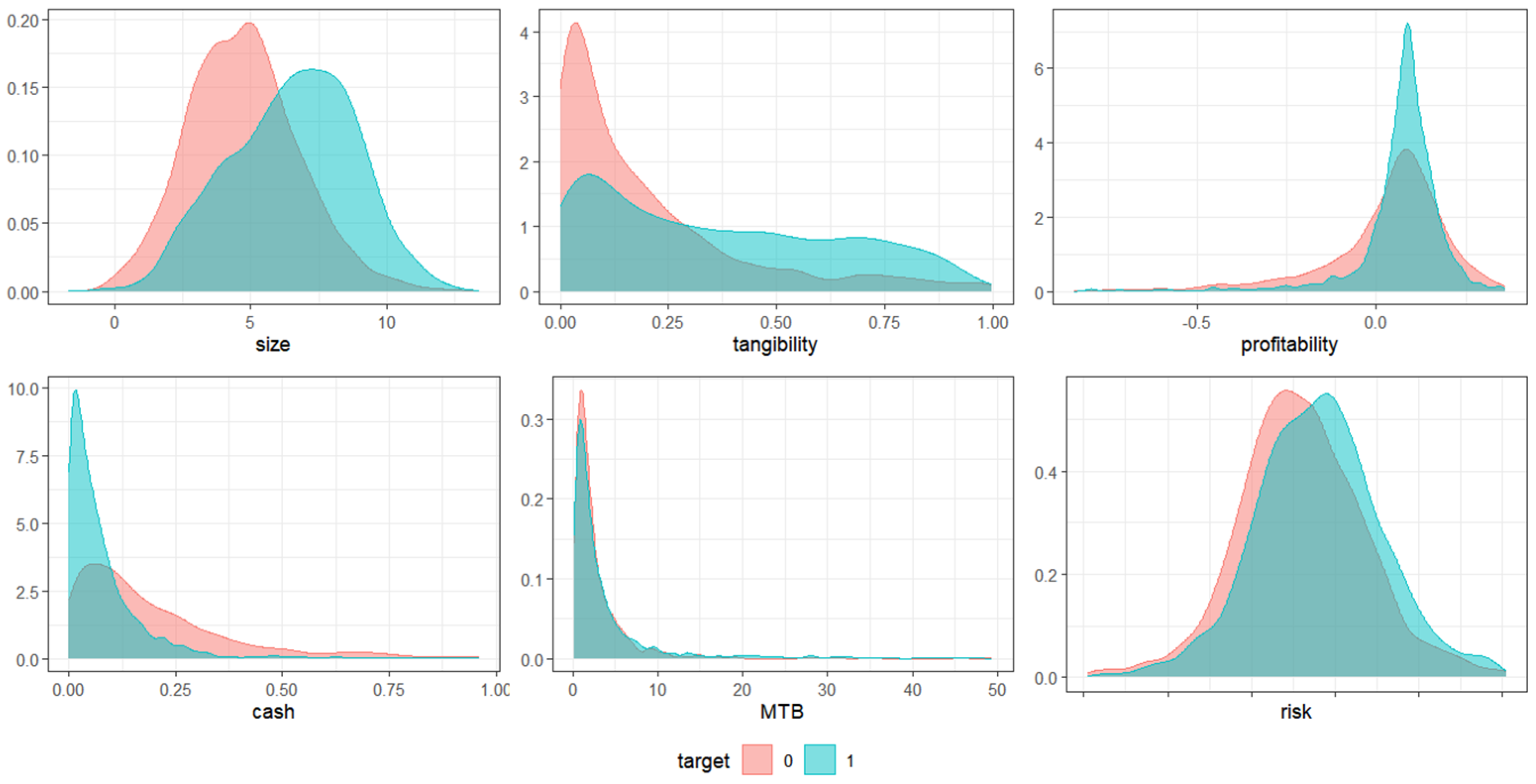
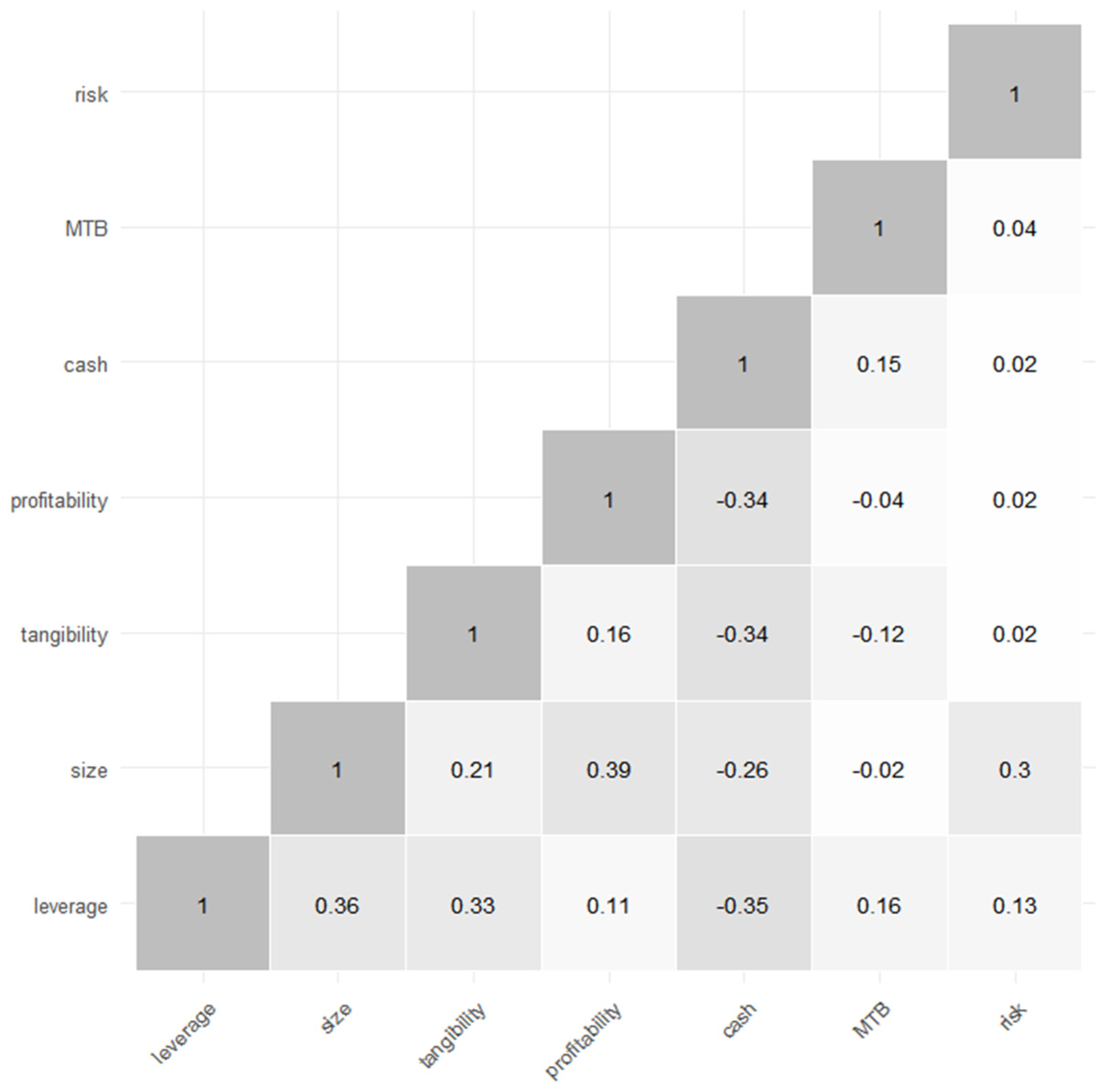
After the initial cleaning stage, the variables used in the models were created. The variable “leverage” is the ratio of total debt to total assets, reflecting the proportion of debt in a company’s financing structure. The variable “size” was obtained using the natural logarithm of total assets, allowing for better scaling in the analysis. “Tangibility” was defined as the ratio of net tangible assets (net value of PP&E) to total assets, indicating the proportion of physical assets in the company’s structure. The variable “profitability” was calculated as the ratio of EBITDA to total assets, reflecting operational efficiency. The “cash” variable was derived as the ratio of cash and cash equivalents to total assets, while “MTB” (market-to-book) was defined as the ratio of market capitalization to total equity, measuring the market value relative to book value and aiming to measure firms’ growth opportunities. Lastly, the “risk” variable was directly obtained from the beta coefficient of the company’s shares.

To further refine the dataset and ensure the integrity of subsequent analyses, an additional cleaning step was performed, focusing on the exclusion of extreme values and outliers based on the variables. This was performed by filtering the variables “profitability”, “MTB”, and “risk” based on the 1st and 99th percentiles. Only records with values within these specified ranges were retained in the dataset. This step was crucial to prevent distortions caused by atypical observations, ensuring that all future analyses would be robust and reliable.

A binary target variable has been created to classify companies into two groups based on their “leverage”. Companies with “leverage” below or equal to the 25th percentile were classified as target = 0 (“low debt level”), while companies with “leverage” above or equal to the 75th percentile were classified as target = 1 (“high debt level”). The companies that fell between these percentiles were excluded. The criterion is justified, as the goal was to select the least and most leveraged companies in the sample based on the first and third quartiles of the “leverage” to maintain a clear binary classification.

As the last cleaning procedure, SIC classifications were cleaned by retaining only categories with at least 10 observations in the dataset to present a minimum representative number of companies in each industry classification. It is worth noting that the threshold of 10 companies represents nearly 1% of the study’s test sample and was chosen as the reference. Dummy variables were created for the SIC variable, transforming the classification into a binary format suitable for machine learning models.

After the whole process of cleaning the dataset, 3.512 companies remain in the sample. The complete sample was then randomly split into training (70%) and test (30%) sub-samples. All continuous feature variables (“size”, “tangibility”, “profitability”, “cash”, “MTB”, “risk”) were standardized in both the training and test datasets. This standardization scaled each variable to have a mean of zero and a standard deviation of one, ensuring comparability across features.

The scripts used in the analyses can be accessed in the Supplementary Materials.

3.3. Supervised Machine Learning Classification Models

Classification models are supervised machine learning algorithms used to predict categories or classes of data [29]. They are trained on labeled datasets to learn patterns that relate input features to their corresponding categories [30,31]. These models are suitable for the purposes of this study, as the objective is to develop a predictive model to classify companies into two subgroups: high levels of debt and low levels of debt. To perform this classification, variables representing the economic and financial status of these companies, as well as other relevant predictive characteristics, are used.

There are two types of learning in classification models: lazy and eager. Eager learners are machine learning algorithms that first build a model from the training dataset before making any prediction on future datasets. They spend more time during the training process in order to achieve better generalization by learning the weights during training, but they require less time to make predictions [32]. Lazy learners, or instance-based learners, on the other hand, do not create a model immediately from the training data. They memorize the training data, and whenever a prediction is needed, they search for the nearest neighbor from the entire training dataset, making them very slow during prediction [33]. For this study, classification models that are eager learners are used, dividing the dataset into training and testing subsets in a 70/30 proportion [34].

Furthermore, there are different types of classification tasks in machine learning models: binary, multi-class, multi-label, and imbalanced classification [30,35]. In this study, binary classification is considered. In a binary classification task, the goal is to classify input data into two mutually exclusive categories (i.e., “event” and “nonevent”) [35,36]. The training data in this study are labeled in a binary format to represent high or low levels of debt in the capital structure of the firms.

Finally, several algorithms are used to estimate binary classification models, and these can be broadly categorized into deterministic models and models based on stochastic simulation. Deterministic models, such as logistic regression (GLM class) and multilevel logistic regression (GLMM class), follow a predefined mathematical structure and yield consistent results for the same input data, as they rely on explicit assumptions about the underlying relationships between variables [29,30,35]. Stochastic-based models, on the other hand, use algorithms that incorporate random components during training, making them flexible and capable of capturing complex patterns on non-linear problems [31]. Some examples include decision trees (DT), random forests (RF), Support Vector Machines (SVMs), Artificial Neural Networks (ANNs), and Gradient Boosting (GB) [30,35,37].

A description of each classification model explored in this study will be presented below, highlighting their main characteristics, the parameters used, as well as the R software (v. 4.4.2) packages and their respective versions employed.

3.3.1. Logistic Models

Binary logistic regression models are used when the goal is to estimate the probability of the occurrence of an event defined by $Y$, which is represented in a qualitative dichotomous form ($Y=1$ to describe the occurrence of the event of interest and $Y=0$ to describe the occurrence of the non-event), based on the behavior of explanatory variables [29,30,35]. In other words, if the phenomenon under study is characterized by only two categories, it will be represented by a single dummy variable, where the first category will serve as the reference and indicate the non-event of interest ($dummy=0$), and the other category will indicate the event of interest ($dummy=1$) [29].

Logistic regression models estimate the odds of the event occurring [38], as represented in the general form of Equation (1). $\alpha$ represents the intercept, ${\beta }_j$ are the estimated parameters for each explanatory variable ($j=\mathrm{1,2},\dots ,k$), and $X_j$ represents the explanatory variables, with $i$ denoting a specific observation in the sample ($i=\mathrm{1,2},\dots ,n$, $n$ is the sample size) [29,35].

$$\mathit{ln}\left({\displaystyle \frac{p_i}{1-p_i}}\right)=\alpha +{\beta }_1{X}_{1i}+{\beta }_2{X}_{2i}+\cdots +{\beta }_k{X}_{ki}$$

(1)

Thus, the general expression for the estimated probability of the occurrence of a dichotomous event for an observation can be defined in Equation (2).

$$p_i={\displaystyle \frac{1}{1+e^{-\left(\alpha +{\beta }_1{X}_{1i}+{\beta }_2{X}_{2i}+\cdots +{\beta }_k{X}_{ki}\right)}}}$$

(2)

The model, therefore, can be estimated using maximum likelihood estimation, with the binary logistic regression model estimating the probability of the occurrence of the event under study for each observation [29].

In addition to the binary logistic model, multilevel logistic models can be used when the data structure is hierarchical, meaning data are nested within clusters, which in turn are nested within other clusters [29]. Random effects can be introduced into these models at different levels of the hierarchy [38].

In this article, we will investigate hierarchical linear models with data nested at two levels: company (level 1) and sector (level 2). These models are referred to as HLM2. In such models, the estimated fixed effects parameters indicate the relationship between the explanatory variables and the dependent variable, while the random components can be represented by the combination of explanatory variables and unobserved random terms [29].

For HLM2 models, the right-hand side of Equation (1) must be rewritten. Equation (3) shows the general form of a multilevel logistic model, considering data nested at two levels [29]. In this case, $P_{ij}$ is the probability of the event of interest occurring for observation $i$ in cluster $j$. ${\beta }_{0j}$ is the cluster-specific intercept for cluster $j$, which can vary between clusters. ${\beta }_{kj}$ are the coefficients associated with the explanatory variables $X_{ijk}$, which may include fixed and random effects. $X_{ijk}$ represents the explanatory variables for observation $i$ in cluster $j$.

At level 2, ${\beta }_{0j}={\gamma }_{00}+u_{0j}$, where ${\gamma }_{00}$ is the fixed effect and $u_{0j}$ is the random effect associated with cluster $j$. ${\beta }_{kj}={\gamma }_{k0}+u_{kj}$, where ${\gamma }_{k0}$ is the fixed effect for the $k$-th explanatory variable, and $u_{kj}$ is the random effect associated with cluster $j$. Substituting these level 2 equations into the level 1 logistic regression, we obtain the full multilevel logistic model with fixed and random effects across two hierarchical levels [29].

$$\mathit{ln}\left({\displaystyle \frac{p_i}{1-p_i}}\right)=({\gamma }_{00}+u_{0j})+\sum _{k=1}^K\left({\gamma }_{k0}+u_{kj}\right)X_{ijk}$$

(3)

To obtain the general expression for the estimated probability of the occurrence of a dichotomous event for an observation, given Equation (3) of the HLM2 multilevel logistic model, it is sufficient to use the fundamental property of the natural logarithm, allowing for a general expression analogous to Equation (2) for the multilevel model.

Logistic regression is easy to implement and interpret, efficient in training, and enables inference about feature importance. It performs well on low-dimensional data, especially when features are linearly separable, and provides well-calibrated probabilities along with classification results [29,36]. However, it is prone to overfitting in high-dimensional data, cannot handle non-linear problems due to its linear decision boundary, and fails to capture overly complex relationships [35].

In order to estimate the mentioned models, the following packages were used in R software: For the logistic regression model, the “glm” function from the “stats” package (v. 4.1.1) was used; for the multilevel logistic regression, the “glmmTMB” package (v. 1.1.10) was used. In this study, only random effects for intercept were applied in the multilevel logistic regression estimation.

3.3.2. Decision Trees (DT)

A decision tree is a non-parametric supervised learning algorithm used for both classification and regression tasks. It features a hierarchical structure that includes a root node, branches, internal nodes, and leaf nodes. The objective is to develop a model that forecasts the target variable’s value by deriving straightforward decision rules from the data’s features [39].

The learning process of a decision tree employs a divide-and-conquer strategy, using a greedy search to find the best split points within the tree. This splitting process is repeated recursively from the top down until most or all records are classified into specific class labels [35,40].

One advantage of decision trees is their ease of interpretation. Their Boolean logic and visual representations make them straightforward to understand and consume. The hierarchical structure also highlights the most important attributes. Additionally, decision trees require little to no data preparation, making them more flexible than other classifiers. They can handle various data types—both discrete and continuous—and can convert continuous values into categorical ones using thresholds. Furthermore, decision trees are versatile as they can be used for both classification and regression tasks. They are also insensitive to underlying relationships between attributes, meaning that if two variables are highly correlated, the algorithm will only choose one to split on [41].

However, decision trees have some disadvantages. They are prone to overfitting, especially when complex, and may not generalize well to new data. They are also high variance estimators, meaning small variations in the data can lead to very different trees. Additionally, the greedy search approach during construction can make them more expensive to train compared to other algorithms [39].

To fit the model, the “rpart” package (v. 4.1.23) was used and based on Gini Index to calculate the node impurity and perform the splits. Additionally, a grid search was performed to select the hyperparameters of the decision tree (e.g., “minsplit”, “maxdepth”, and “minbucket”). The values tested for hyperparameters in the grid search were the following: minsplit (5, 10, 50, 100), maxdepth (3, 5, 10), and minbucket (5, 10, 50, 100). The model with the combination of hyperparameters achieves the lowest cross-validation error after the grid search is selected.

3.3.3. Random Forrest (RF)

A random forest is an advanced ensemble learning method that combines several decision tree classifiers on various sub-samples of the dataset, using averaging to enhance predictive accuracy and mitigate overfitting [42].

Random forest algorithms have three main hyperparameters to set before training: node size, the number of trees, and the number of features sampled. The random forest algorithm consists of a group of decision trees, where each tree in the ensemble is built from a bootstrap sample—a data sample drawn from the training set with replacement. One-third of this training sample is reserved as test data, known as the out-of-bag sample. Another layer of randomness is introduced through feature bagging, increasing dataset diversity and reducing the correlation among decision trees. If the task is classification, the most frequent categorical variable determines the predicted class. Lastly, the out-of-bag sample is employed for cross-validation, finalizing the prediction process [35,40].

Random forests can reduce the risk of overfitting by averaging uncorrelated decision trees, which decreases overall variance and prediction error. The method is also highly flexible, capable of handling both regression and classification tasks with great accuracy, and it can estimate missing values effectively through feature bagging. Additionally, random forests make it easy to determine feature importance using measures such as Gini importance, mean decrease in impurity (MDI), and permutation importance (MDA) [35,40]. However, random forests have some drawbacks. The process can be time-consuming, as generating predictions involves computing each decision tree individually. They also require more resources, both in terms of memory and storage, due to handling large datasets. Lastly, while a single decision tree is easy to interpret, a random forest’s complexity makes its predictions more difficult to understand [41].

The package used to fit the random forest model is the “randomForest” package (v. 4. 7.1.2). The following hyperparameters were explored in the grid search technic: “ntree” (total number of trees), “mtry” (number of variables randomly selected at each node), and “nodesize” (the minimum size of the terminal nodes). The values tested for hyperparameters in the grid search were the following: ntree (500, 1000, 2000), mtry (5, 10, 15), and nodesize (1, 10, 50, 100). The metric used to select the best set of hyperparameters is the error based on the confusion matrix of the fitted model, aiming to select the lowest possible value.

3.3.4. Artificial Neural Networks (ANNs)

A neural network is a machine learning model designed to mimic the decision-making process of the human brain by simulating how biological neurons work together [35]. It has two main uses: clustering (unsupervised classification) and establishing relationships between numeric inputs (attributes) and outputs (targets) [40].

Neural networks consist of layers of nodes (artificial neurons): an input layer, one or more hidden layers, and an output layer. Each node connects to others with associated weights and thresholds. If a node’s output exceeds its threshold, it activates and passes data to the next layer [41]. Common activation functions include Step, ReLU, Sigmoid, and Tanh, which enable the network to interpret non-linear and complex data patterns [40].

Each node functions like a regression model, with inputs, weights, a bias (or threshold), and an output. Inputs are multiplied by their weights, summed, and passed through an activation function, which determines the output. If the result surpasses a threshold, the node activates, sending its output as input to the next node [35].

During training, the model’s accuracy is assessed using a cost (or loss) function. The goal is to minimize this function by adjusting weights and biases through a process called gradient descent [40]. This iterative method helps the model learn the optimal parameters by reducing errors and converging toward a local minimum [35,41].

Configuring an artificial neural network (ANN) involves experimentation with factors like learning rate, decay, momentum, the number of hidden layers, and nodes per layer. This process requires multiple training runs to refine the model [40,41,43].

ANNs offer several advantages, including their ability to handle complex classification problems with numerous parameters, model non-linear relationships efficiently, perform numerical predictions, and work without assumptions about data distribution. However, they have drawbacks, such as slow training and application phases, lack of interpretability, and the absence of hypothesis testing or statistical metrics like p-values for variable comparison [41].

The package used to model the neural network was “neuralnet” (v. 1.44.2). Cross-validation with grid search was performed to find the best hyperparameters. The hyperparameters were tuned in the grid search: “hidden” (number of neurons in the hidden layers). The values tested were one layer with two or three neurons and two hidden layers with two neurons in each one. Cross-validation was conducted by splitting the training data into five folds. The AUC metric was calculated for each fold using the “roc” function from the “pROC” package (v. 1.18.5). The average AUC across the folds was recorded for each hyperparameter. After the grid search, a final model was trained on the complete training data using the chosen configuration, which demonstrated the best performance. The training used the “rprop+” (resilient propagation) algorithm, with a logistic activation function and non-linear output.

3.3.5. Extreme Gradient Boosting (XGBoost)

Gradient Boosting (GB) is an ensemble-supervised machine learning algorithm applicable to both classification and regression tasks. The final model is formed by combining numerous individual models. Gradient Boosting trains these models sequentially, assigning greater weight to instances with incorrect predictions. This ensures that challenging cases receive more focus during training. The process minimizes a loss function incrementally, similar to the weight optimization in Artificial Neural Networks (ANNs) [35,41].

In GB, after weak learners are built, their predictions are compared to actual values. The difference between predictions and actual values represents the model’s error rate. This error is used to calculate the gradient, the partial derivative of the loss function. The gradient indicates the direction in which model parameters should be adjusted to reduce errors in subsequent iterations. Unlike ANNs, where a single model minimizes the loss function, GB combines predictions from multiple models. Consequently, GB uses hyperparameters from random forests, such as the number of trees, along with others, like the learning rate and loss function, typical of ANN models [35,40].

Boosting combines numerous weak learners—models slightly better than random guessing—into a strong learner. These weak learners are trained sequentially to correct errors from previous models, and through numerous iterations, they are transformed into a robust model [35,40,41].

XGBoost, a variant of GB, introduces several enhancements. It employs L1 and L2 regularization to improve generalization and reduce overfitting. Unlike traditional GB, which uses the first partial derivative of the loss function, XGBoost leverages the second partial derivative, providing more detailed information about the gradient’s direction. Additionally, XGBoost is faster due to parallelized tree construction, can handle missing values directly, and requires less data preparation, making it more efficient and scalable [40]. However, XGBoost may underperform when the training dataset has significantly fewer observations than features, and it is not ideal for computer vision, natural language processing, or regression tasks requiring continuous output prediction or extrapolation beyond the training data range. Additionally, XGBoost requires careful parameter tuning for optimal performance, and its complexity can make model interpretation challenging [35].

The package used to estimate the XGBoost model was the “xgboost” package (v. 1.7.8.1). A grid search was conducted to find the best combination of hyperparameters for XGBoost through cross-validation. The following hyperparameters were varied: “eta” (learning rate), “max_depth” (maximum depth), and “nrounds” (number of rounds). The values tested for hyperparameters in the grid search were the following: eta (0.001, 0.01, 0.10), maxdepth (3, 5, 10), and nrounds (100, 500, 1000). Cross-validation was performed using the “xgb.cv” function with 5 folds. The error metric “test_error_mean” was recorded for each combination of hyperparameters, and the configuration with the lowest average error was selected.

3.3.6. Support Vector Machine (SVM)

Support Vector Machines (SVMs) are used for classifying both linear and non-linear data [35]. The SVM algorithm transforms the original training data into a higher-dimensional space using a non-linear mapping. In this space, it identifies an optimal linear separating hyperplane (a decision boundary) to distinguish between two classes. The SVM leverages support vectors—key data points that define the margins—and aims to maximize the distance between these support vectors through the hyperplane [40,43]. The cost parameter controls the model’s complexity: a high cost results in a more flexible model prone to overfitting, while a low cost leads to a stiffer model that reduces overfitting but risks underfitting due to a stronger influence of squared parameters in the error function [35].

SVMs are a powerful supervised learning algorithm with several advantages, such as effectively handling high-dimensional data, small datasets, and non-linear decision boundaries using the kernel trick [35,40,43]. SVMs are robust to noise, provide good generalization performance, and offer efficient sparse solutions by using only a subset of training data [41]. They can be applied to various tasks, including classification and regression [35]. However, SVMs have limitations: they are computationally expensive for large datasets, sensitive to parameter choices, and the choice of kernel significantly affects performance. SVMs also struggle with overlapping classes, large datasets with many features, and missing values while lacking a probabilistic interpretation of decision boundaries [35].

The SVM model was implemented using the “svm()” function from the “e1071” package (v. 1.7.16). Initially, a grid search was conducted with the “tune.svm()” function to find the optimal combination of the hyperparameters “cost” and “gamma”. The values tested for hyperparameters in the grid search were the following: cost (0.01, 0.1, 1, 10, 100) and gamma (0.01, 0.1, 1, 10, 100). Additionally, cross-validation with five folds was performed, specified by the “tune.control(cross = 5)” command. The main arguments used in the SVM model were type = “C-classification” (for supervised classification problems), kernel = “radial” (a radial kernel effective for non-linear problems), “cost” (penalty for misclassified samples), “gamma” (influence of samples on the radial kernel decision calculation), and “scale” = FALSE (no variable standardization is applied) because the data were already standardized.

3.4. Model Performance Assessment

There are several evaluation metrics for classification models, depending on the specific task performed, making it important to assess the model’s performance and its ability to generalize to new data [35]. For the binary classification models used, the main metrics are Accuracy, Precision, Sensitivity, Specificity, F1-score, Confusion matrix, and AUC-ROC [44,45].

The confusion matrix is a 2 × 2 matrix that summarizes the number of correct predictions made by the model and also helps in calculating other metrics [45]. The confusion matrix contains 4 elements: true positives (TP) are the data samples that the model correctly predicts in their respective class; false positives (FP) are the negative-class instances incorrectly identified as positive cases; false negatives (FN) are actual positive instances erroneously predicted as negative; and true negatives (TN) are the actual negative class instances that the model accurately classifies as negative [35]. False positives are classified as Type 1 errors, while false negatives are classified as Type 2 errors [44].

Accuracy provides the number of correct predictions made by the model [45]. Accuracy gives a high-level overview of a model’s performance but does not reveal if a model is better at predicting certain classes over others [35]. It is calculated by dividing the sum of true positives and true negatives by the total number of predictions [44].

Precision is the proportion of predictions for the positive class that actually belong to that class [45]. In this sense, precision reveals whether a model is correctly predicting the target class [35]. This metric is calculated by dividing the sum of true positives by the total number of positive predictions [44].

Sensitivity indicates how good the model is at predicting events in the positive class, also known as the true positive rate [35]. In other words, sensitivity shows how often a model detects members of the target class in the dataset, calculated by dividing true positives by the sum of true positives and false negatives [44]. Specificity, on the other hand, indicates how good the model is at predicting events in the negative class (true negative rate) [35]. In other words, specificity shows how often a model detects members of the non-target class in the dataset, calculated by dividing true negatives by the sum of true negatives and false positives [44].

The F1-score combines the precision and sensitivity metrics by calculating their harmonic mean [45]. This metric is particularly useful in imbalanced datasets, where one class may dominate the other, as it accounts for both false positives and false negatives, offering a more comprehensive evaluation of the model’s ability to correctly predict both classes [44].

Considering that the confusion matrix depends on the establishment of a cutoff to classify observations into a category (event or non-event), in this study, the cutoff of 50% was used. Therefore, if an ML model estimates that the probability of an observation being “event” is greater than 50%, then the observation will be classified as an “event”. Otherwise, it will be classified as a non-event.

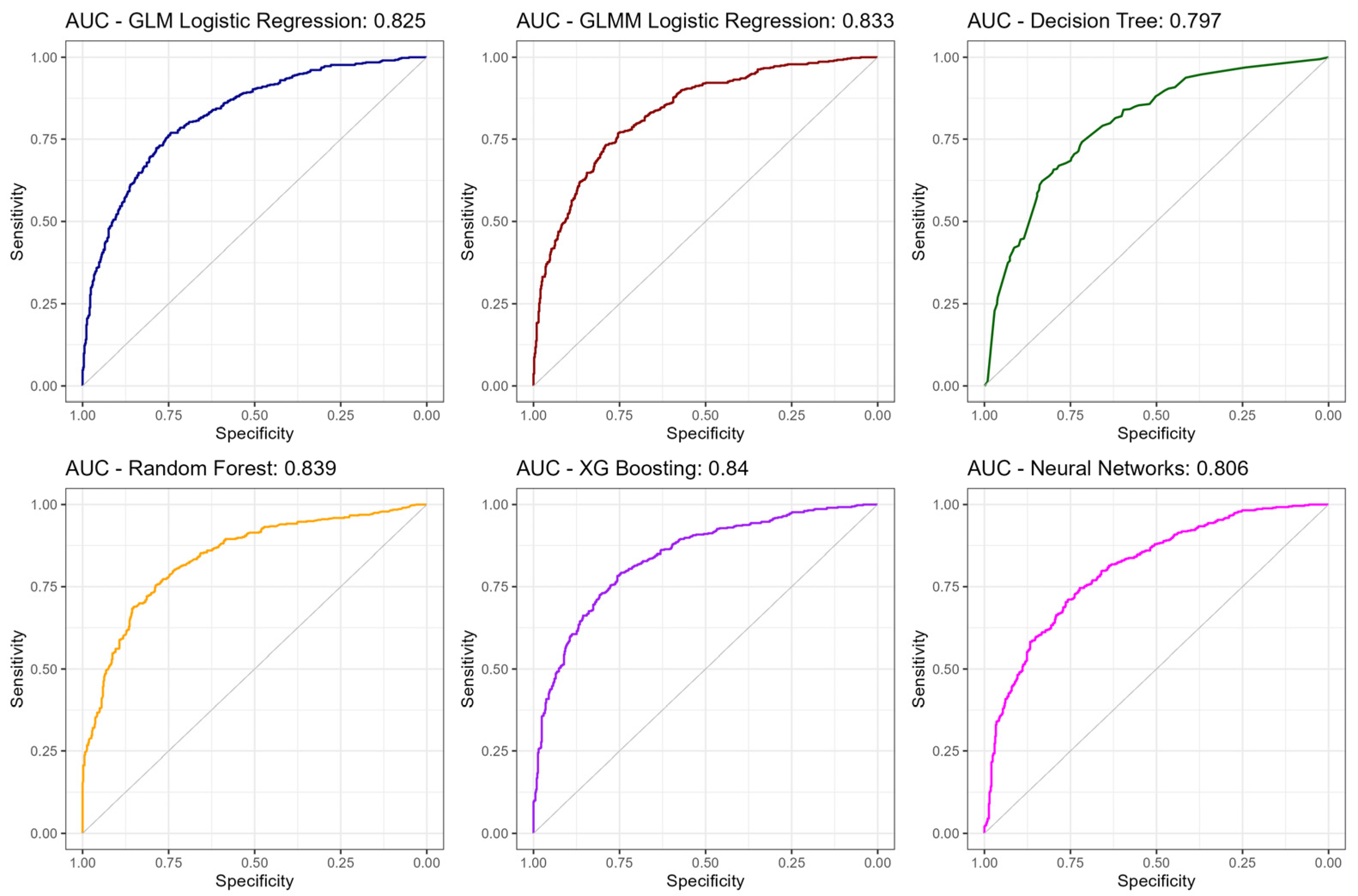
Finally, the AUC-ROC is the area under the ROC curve. The ROC curve plots the true-positive rate (i.e., the sensitivity) against false-positive rate (one minus the specificity) for different decision thresholds (cutoff points to transform probabilities into classes), showing the model’s performance at various thresholds [29,35]. The area under the curve quantifies this performance, with an AUC of 0.5 representing a random model and an AUC of 1 indicating a perfect model [45].

4. Results and Discussions

4.1. Descriptive Analysis of the Dataset

The processed database, after the procedures described in Section 3.2, contains the following feature variables: “size”, “tangibility”, “profitability”, “cash”, “MTB”, “risk”, and all the dummy variables associated with the SIC variable, totaling 54 dummies. Therefore, in total, there are 60 explanatory variables. The dependent binary variable is “target”. The processed database contains a total of 3512 observations. Table 1 shows the descriptive statistics of the continuous explanatory variables for the full sample.

Table 1. Descriptive statistics—sample of both groups (high and low debt).

Sample of High and Low Groups Together
	Min	1st Quart	Median	Mean	sd	3rd Quart	Max	obs
leverage	0.0000	0.0343	0.0952	0.2556	0.2312	0.4464	0.9423	3512
size	−1.669	3.886	5.545	5.637	2.3472	7.343	13.382	3512
tangibility	0.0000	0.0566	0.1849	0.2782	0.2646	0.4491	0.9972	3512
profitability	−0.8435	0.0152	0.0812	0.0514	0.1504	0.1309	0.3625	3512
cash	0.0000	0.0304	0.0822	0.1362	0.1588	0.1808	0.9598	3512
MTB	0.1312	0.9233	1.7498	3.2761	4.8945	3.5688	49.4258	3512
risk	−1.9536	0.2099	0.6938	0.7059	0.7680	1.1932	3.0572	3512

Considering the purpose of classifying companies into high- or low-debt groups, descriptive statistics are also presented for each group separately below. The first and third quartiles of the “leverage” variable were used as the basis for separating the two groups. The first quartile of the variable is 0.0953, and the third quartile is 0.3394. It is worth noting that these reference quartiles are of the variable before the selection of firms and the formation of the groups. Therefore, all companies that present “leverage” less than or equal to 0.0953 were classified in the “low debt” group (target = 0), and all companies that present leverage greater than or equal to 0.3394 were classified in the “high debt” group (target = 1).

Due to this criterion, the groups are very balanced in terms of the number of observations. There are 1753 companies in the “high debt” group and 1759 companies in the “low debt” group. The descriptive statistics for each group are presented on Table 2 and Table 3.

Table 2. Descriptive statistics—“high debt” group.

High Debt Level (Target = 1)
	Min	1st Quart	Median	Mean	sd	3rd Quart	Max
leverage	0.3394	0.3858	0.4467	0.4731	0.1086	0.5356	0.9423
size	−0.6266	4.9222	6.7100	6.5403	2.2915	8.2591	13.3822
tangibility	0.0000	0.1048	0.3134	0.3619	0.2791	0.5967	0.9858
profitability	−0.8015	0.0423	0.0870	0.0700	0.1224	0.1288	0.3564
cash	0.0000	0.0184	0.0494	0.0798	0.1035	0.1000	0.9445
MTB	0.1371	0.9161	1.8077	3.7913	5.8965	3.9087	47.3827
risk	−1.9475	0.3133	0.8107	0.8083	0.7599	1.2738	3.0057

Table 3. Descriptive statistics—“low debt” group.

Low Debt Level (Target = 0)
	Min	1st Quart	Median	Mean	sd	3rd Quart	Max
leverage	0.0000	0.0095	0.0344	0.0389	0.0302	0.0661	0.0953
size	−1.669	3.316	4.684	4.736	2.0357	5.960	12.764
tangibility	0.0000	0.0356	0.1161	0.1947	0.2197	0.2650	0.9972
profitability	−0.8435	−0.0243	0.0679	0.0328	0.1718	0.1346	0.3625
cash	0.0000	0.0618	0.1363	0.1923	0.1827	0.2617	0.9598
MTB	0.1312	0.9354	1.6831	2.7626	3.5589	3.3283	49.4258
risk	−1.9536	0.1245	0.5788	0.6039	0.7627	1.0859	3.0572

Based on the statistics, companies are, on average, considerably different between the two groups. Firstly, due to the operational definition of the target binary variable, companies in the “high debt” group are considerably more leveraged, so that, on average, 47.31% of their assets are financed with debt, compared to only 3.89% in the low debt group.

Therefore, regarding the target variable, the sample companies are well separated, which can prevent misclassifications of the ML models due to very similar leverages. In this context, companies financing with a higher proportion of debt do so with an important difference in relation to the other group.

In terms of the firms’ features, sample companies are also different. Companies in the “high debt” group are, on average, larger, have a greater tangibility of assets, are more profitable, have lower cash holdings, have greater growth opportunities, and are riskier. This evidence may indicate that the characteristics of the companies may be important predictors of debt financing and may serve as relevant predictor variables for classifying firms into groups in the supervised ML models.

Next, the density plots of the firms’ variables (Figure 1) show that the differences are not only on average, especially for size, tangibility, profitability, and cash variables. On the other hand, the distribution of the “MTB” and “risk” variables is more similar between the groups.

Figure 1. Density plots of the firms’ variables.

The Pearson correlation coefficients are presented in Figure 2 and show that the largest positive correlations are between “leverage” and “size” and “leverage” and “tangibility”. The correlation between “leverage” and “cash” is the largest negative coefficient. In unreported coefficients significance p-values, it is noted that all correlation coefficients between leverage and companies’ features are statistically significant at the 95% confidence level, corroborating that these attributes can serve as good predictors of debt financing in ML classification models.

Figure 2. Pearson correlation matrix.

The results of the supervised ML classification models are presented below for both the training and test samples. The hyperparameters selected in the grid search procedures of the stochastic models were the following: decision tree (“minsplit” = 5; “maxdepth” = 10; “minbucket” = 10), random forest (“ntree” = 1000, “mtry” = 15, “nodesize” = 50), XGBoost (“eta” = 0.10; “max_depth” = 3; “nrounds” = 500), neural network (“hidden” = 2), and SVM (“cost” = 10; “gamma” = 0.01). These were the values that generated the best results for the evaluation metrics among those tested.

4.2. Classification Models

For each model, performance evaluation metrics were obtained for the training sample (Table 4) and the test sample (Table 5). The following metrics were used: accuracy, precision, sensitivity, specificity, F1-score, and AUC-ROC. Additionally, the values from the confusion matrix (TP, FP, TN, and FN) are presented, which allow for the determination of Type 1 and Type 2 errors.

Table 4. Results—train sample.

Metric	GLM 1	GLMM 2	DT	RF	XGBoost	SVM	ANN
Accuracy	76.16%	76.12%	82.30%	83.44%	90.03%	77.46%	78.89%
Precision	76.48%	76.12%	82.82%	83.63%	90.29%	77.24%	79.30%
Sensitivity	76.23%	76.79%	81.95%	83.56%	89.93%	78.49%	78.73%
Specificity	76.09%	75.43%	82.66%	83.32%	90.14%	76.42%	79.05%
F1-Score	76.35%	76.45%	82.38%	83.59%	90.11%	77.86%	79.01%
TP	946	953	1017	1037	1116	974	977
FP	291	299	211	203	120	287	255
TN	926	918	1006	1014	1097	930	962
FN	295	288	224	204	125	267	264
AUC-ROC	0.844	0.840	0.885	0.928	0.967	-	0.875

¹ Binary logistic model; ² multilevel logistic model (HLM2).

Table 5. Results—test sample.

Metric	GLM 1	GLMM 2	DT	RF	XGBoost	SVM	ANN
Accuracy	75.24%	75.90%	72.20%	76.94%	76.19%	75.81%	73.06%
Precision	74.75%	74.62%	71.94%	76.12%	74.86%	74.66%	72.01%
Sensitivity	74.02%	76.37%	70.12%	76.56%	76.76%	75.98%	72.85%
Specificity	76.38%	75.46%	74.17%	77.31%	75.65%	75.65%	73.25%
F1-Score	74.38%	75.48%	71.02%	76.34%	75.80%	75.31%	72.43%
TP	379	391	359	392	393	389	373
FP	128	133	140	123	132	132	145
TN	414	409	402	419	410	410	397
FN	133	121	153	120	119	123	139
AUC-ROC	0.825	0.833	0.797	0.838	0.840	-	0.806

¹ Binary logistic model; ² multilevel logistic model (HLM2).

To illustrate the AUC-ROC values presented in Table 5 for the test sample, Figure 3 displays the ROC curves for the explored models, along with the corresponding area under the curve values.

Figure 3. AUC-ROC—logistic, multilevel logistic, DT, RF, XG boosting, and ANN.

Comparing the results of the models in the training sample (Table 4), XGBoost was the one that best classified the companies with 90.03% accuracy. Next, RF and DT appear, indicating the best performance of the tree-based models in this training sample. Even taking the AUC-ROC as the basis of comparison, a metric that does not depend on a cutoff, these models stand out among the others. In common, XGBoost and RF techniques both benefit from the aggregation of several individual predictors (decision trees) to obtain a consolidated final prediction with better expected quality. The better quality of the predictions of the ensemble models is evident when compared with the predictions of the individual decision tree, which showed lower accuracy even in the training sample.

When the three models are compared based on the accuracy confidence interval (Table 6) for the training sample, XGBoost stands out as the best among them. DT and RF can be considered indistinguishable from this perspective.

Table 6. A 95% confidence interval for accuracy in training and test samples.

Accuracy 95% CI
	Train Sample		Test Sample
GLM	0.7442	0.7783	0.7252	0.7782
GLMM	0.7438	0.7779	0.732	0.7846
DT	0.8074	0.8379	0.6939	0.7489
RF	0.8191	0.8489	0.7428	0.7946
XGBoost	0.8878	0.9119	0.735	0.7873
SVM	0.7576	0.791	0.731	0.7836
ANN	0.7722	0.8048	0.7027	0.7571

The other measures from the confusion matrix (precision, sensitivity, specificity, and F1-score), as can be seen in Table 4, do not show large differences in relation to the accuracy of the model. This means that the ML models did not make asymmetrical mistakes when classifying the two classes (high or low debt levels) in the models.

In the training sample (Table 4), the two models with deterministic estimation, i.e., logistic regression and multilevel logistic regression, presented the lowest accuracy and AUC-ROC, although they are comparable to neural networks and SVM. It is worth noting that the SVM does not present an AUC-ROC curve, as the algorithm does not generate predictions in terms of probabilities and only generates the event or non-event prediction.

When comparing the results in training and test samples (Table 4 and Table 5), accuracy indicates that DT, RF, and XGBoost excelled in the training phase but also showed higher levels of overfitting, given that in the test sample, they cannot achieve the same performance. They are great predictors in the training sample, but the accuracy drops considerably in the test sample. Using accuracy for comparison, the deterministic logistic models presented the lowest level of overfitting. Although these models did not perform better than the others in the test sample, evidence indicates that they do not overfit in the training sample.

Additionally, considering the accuracy of the models, and when considering their confidence interval (Table 6), all estimated models performed the same on the test sample. This means that, in terms of overall effectiveness in generalizing the results of the model, all models present results that are not statistically different. In this case, considering the generalization of the models’ results, they all present similar measures. A similar result is found when using the AUC-ROC as a reference, as can be seen in Figure 3.

Considering that the results may depend on the choice of the categorization of the dependent variable based on the first and fourth quartile of the “leverage”, as a robustness check, the 15th and 85th percentiles were also tested to generate the debt level groups. The results (not reported) were qualitatively the same.

In addition to the performance evaluation metrics, the DT, RF, and XGBoost models allow for the determination of the relative importance of variables. The plots generated for each of these models can be seen in Figure 4, Figure 5 and Figure 6, respectively.

Figure 4. Variable importance—decision tree.

Figure 5. Variable importance—random forest.

Figure 6. Variable importance—XGBoosting.

Through the analysis of Figure 4, Figure 5 and Figure 6, it is observed that some variables consistently maintain high relative importance regardless of the model. These include mainly “size”, “cash”, and “tangibility” as the three main variables. In general, firms’ characteristics are consistently important in the models. However, the dummy variables for SIC, which classify the company’s economic activities, exhibit low relative importance in these models.

Nevertheless, this study did not focus on selecting the most significant variables; all variables were utilized and retained in the models, regardless of their relative importance. The figures presented, therefore, aim to provide insights into which variables carry the most weight in the models.

5. Conclusions

This study investigated the use of supervised machine learning models to classify companies into two distinct groups based on their debt levels (high and low levels). Through the analysis of different classification models—encompassing both deterministic and stochastic algorithms—metrics such as accuracy, precision, sensitivity, specificity, F1-score, and AUC-ROC were evaluated to identify the most effective approaches for the proposed task.

The results indicated that tree-based models, such as DT, RF, and XGBoost, demonstrated the highest performances in the training sample, with higher accuracy and AUC-ROC. However, they exhibited signs of overfitting, as their performance in the test sample was significantly lower than in the training phase compared to the other models. In contrast, deterministic models, such as logistic regression and multilevel logistic regression, showed a lower risk of overfitting, though their overall performance was inferior to stochastic models in the training sample.

A noteworthy finding was that, in the test sample, all approaches delivered statistically similar results in terms of overall effectiveness. This suggests that, although the aforementioned tree-based models stood out in specific metrics, the choice of the optimal model should consider the balance between performance, simplicity, and interpretability.

Furthermore, the results underscore the importance of variables such as company size, tangibility, profitability, liquidity, growth opportunities, and risk as relevant predictors of corporate capital structure. These variables not only differentiated the groups of high- and low-debt companies but also significantly influenced the models’ performance.

Thus, the evidence presented in this study can contribute to managerial decision-making, providing a practical reference for classifying companies in terms of capital structure. Machine learning-based tools can help managers identify the need for adjustments in debt strategies, fostering more informed decisions aligned with company characteristics and finance structure.

Finally, future research could explore different preprocessing approaches, expand the analysis to include other explanatory variables or investigate the application of models in different economic contexts and sectors. Additionally, future studies could explore the consideration of a continuous leverage variable, using models different from the binary classification models employed here, similar to the model proposed by [46]. Furthermore, for future studies comparing different classification models and continuous dependent variables, it is worth exploring other performance evaluation metrics for the models, according to the S.A.F.E. methodology proposed by [47]. Finally, there are studies that demonstrate the importance of the explainability of the results obtained in ML models through explainable artificial intelligence (XAI) methods, which can help both in the selection of relevant explanatory variables for the models and in the comparison of the results [48,49,50]. Although the focus of this study was primarily on accuracy and AUC-ROC, the trade-off between predictive accuracy and explainability in ML models is a relevant discussion for future applications that address the financing of the companies. It is hoped that this work will serve as a foundation for further investigations into the use of artificial intelligence in analyzing corporate capital structure.