On the Pricing of Vulnerable Foreign Equity Options with Stochastic Volatility in an Intensity-Based Model

Abstract

In this study, we investigate the pricing of two types of vulnerable foreign equity options using an intensity-based model. It is considered that the intensity process consists of both systematic and idiosyncratic components. In addition, we assume that the underlying asset processes follow a two-factor stochastic volatility model. Under the proposed model, we obtain the explicit pricing formulas of vulnerable foreign equity options. Finally, we provide some numerical examples to demonstrate how credit risk and stochastic volatility affect option prices.

1. Introduction

The suitable valuation of financial derivatives with credit risk has become increasingly important since the 2008 global financial crisis, which exposed the potential risks of underestimating counterparty risk. While the Black–Scholes model [1] is the basis of option pricing, the assumption of risk-free counterparties has proven insufficient, especially in over-the-counter (OTC) markets, where credit risk occurs in each transaction. In other words. as OTC markets have increased in size and complexity, incorporating credit risk into derivative pricing has become not only important but essential.

Two main approaches for modeling credit risk in options were developed: structural models and intensity-based (reduced-form) models. The structural models, developed by Johnson and Stulz [2] and expanded by Klein [3], define default as occurring when the counterparty’s assets fall below a predetermined threshold. While obvious, structural models have limitations due to the assumption that a firm’s asset value is observable and the difficulty of capturing unexpected defaults. Jarrow and Turnbull [4] proposed intensity-based models, which were later extended by Lando [5], providing an alternative model in which default is considered an exogenous event governed by the Cox process. This approach has several advantages; it better demonstrates the unpredictable character of defaults, allows for more flexible correlation structures, and frequently results in more tractable mathematical expressions. In addition, intensity-based models can better incorporate market data from credit default swaps and corporate bonds. In this paper, we consider an intensity-based model to model the credit risk.

Our study provides an alternative approach for foreign equity options with credit risk, a popular but understudied type of exotic derivative. Kwok and Wong [6] first provided the pricing formulas of different foreign equity options under the Black–Scholes model based on the partial differential equation (PDE) approach. Meanwhile, foreign equity options have been extensively studied since Kwok and Wong’s primary work, with extensions to the Lévy process [7], stochastic volatility [8,9], regime switching [10], and jump diffusion [11,12]. Several recent studies have focused on the valuation of foreign equity options while considering the credit risk of the counterparty. Kim et al. [13] used Mellin transforms to solve the PDEs for the prices of foreign equity options with credit risk under the structural model. Kim [14] derived the pricing formulas of vulnerable foreign equity options in the intensity-based model using the mean-reverting OU process for the intensity process based on Fard’s model [15] by employing the probabilistic approach. However, these studies have limitations because they used the Black–Scholes model. In this paper, we develop the model for pricing vulnerable foreign equity options using stochastic volatility models, which describe the volatility smile in the real market. Furthermore, we adopt an adequate intensity-based approach to model the credit risk of vulnerable foreign equity options. We describe the stochastic default intensity using a Cox–Ingersoll–Ross (CIR) process, which allows for mean reversion in credit risk while remaining analytically tractable. This captures the empirically observed clustering of defaults and the temporal variability of credit risk.

The remainder of this paper is structured as follows. Section 2 describes our model framework and introduces two types of vulnerable foreign equity options. Section 3 presents the analytical pricing formulas of the options. Section 4 provides some numerical examples. Finally, Section 5 offers some concluding remarks.

2. Model

We assume that $S_f\left(t\right)$ and $S_d\left(t\right)$ are the prices of foreign and domestic stocks, respectively. The relation between $S_f\left(t\right)$ and $S_d\left(t\right)$ can be described as $S_d\left(t\right)=F\left(t\right)S_f\left(t\right)$, where $F\left(t\right)$ denotes the exchange rate in the domestic currency per unit of foreign currency at time t. We also assume that the risk-neutral dynamics $S_f\left(t\right)$ and $F\left(t\right)$ in foreign currency, which have two-factor stochastic volatility, are given by

$$\begin{array}{c}\frac{d{S}_f\left(t\right)}{S_f\left(t\right)}=r_{f}dt+{\sigma }_S\sqrt{v_1\left(t\right)}d{W}_1\left(t\right)+\sqrt{v_2\left(t\right)}d{W}_2\left(t\right),\hfill \\ \hfill \mathrm{(1)}& \frac{dF\left(t\right)}{F\left(t\right)}=(r_f-r_d)dt+{\sigma }_F\sqrt{v_1\left(t\right)}d{W}_1\left(t\right)+\sqrt{v_3\left(t\right)}d{W}_3\left(t\right),\hfill \end{array}$$

where ${\sigma }_S$ and ${\sigma }_F$ are constants, $W_i\left(t\right)$ $(i=1,2,3)$ represents standard Brownian motions, and $r_d$ and $r_f$ denote the domestic and foreign risk-free interest rates, respectively. In addition, we have

$$\begin{array}{c}\hfill d{v}_i\left(t\right)=(a_i-b_i{v}_i\left(t\right))dt+{\gamma }_i\sqrt{v_i\left(t\right)}d{B}_i\left(t\right),(i=1,2,3)\end{array}$$

(2)

where $a_i,b_i,{\gamma }_i$ $(i=1,2,3)$ are constants and $B_i\left(t\right)$ $(i=1,2,3)$ represents the standard Brownian motions. The standard Brownian motions mentioned above have the following correlations:

$$d{W}_1\left(t\right)d{B}_1\left(t\right)={\rho }_{1}dt,d{W}_2\left(t\right)d{B}_2\left(t\right)={\rho }_{2}dt,d{W}_3\left(t\right)d{B}_3\left(t\right)={\rho }_{3}dt,$$

and other Brownian motions are pairwise independent. Then, under the domestic risk neutral measure Q, the dynamics in a domestic currency are represented by

$$\begin{array}{c}\frac{d{S}_f\left(t\right)}{S_f\left(t\right)}=(r_f-{\sigma }_S{\sigma }_F{v}_1\left(t\right))dt+{\sigma }_S\sqrt{v_1\left(t\right)}d{W}_1\left(t\right)+\sqrt{v_2\left(t\right)}d{W}_2\left(t\right),\hfill \\ \mathrm{(3)}& \frac{dF\left(t\right)}{F\left(t\right)}=(r_d-r_f)dt+{\sigma }_F\sqrt{v_1\left(t\right)}d{W}_1\left(t\right)+\sqrt{v_3\left(t\right)}d{W}_3\left(t\right).\hfill \end{array}$$

In the following, we consider an intensity-based model for modeling the credit risk of an option issuer. As in the work by Wang [16], we assume that the intensity process is divided into two parts. The first part examines systematic risk, while the second examines the idiosyncratic risk of option issuers. Then, the intensity process is defined by

$$\lambda \left(t\right)=\beta v_1\left(t\right)+v\left(t\right),$$

where $\beta$ is is a nonnegative constant and $v\left(t\right)$ describes the idiosyncratic risk, defined by

$$\begin{array}{c}\hfill dv\left(t\right)=(a-bv\left(t\right))dt+\gamma \sqrt{v\left(t\right)}dB\left(t\right),\end{array}$$

(4)

where $a,b,\gamma$ are constants and $B\left(t\right)$ is a standard Brownian motion independent of all other Brownian motions. Then, the default $\tau$ is defined by

$$\mathrm{P}\left(\tau >t\right)=\mathrm{E}\left[e^{-{\int }_0^t\lambda \left(s\right)ds}\right],$$

where $0<t\le T$ and T is the time to maturity.

In this paper, we consider two kinds of foreign equity options:

(1)

The payoff of foreign equity call struck in foreign currency:

$$F\left(T\right){(S_f\left(T\right)-K_f)}^{+}$$

(2)

The payoff of foreign equity call struck in domestic currency:

$${(F\left(T\right)S_f\left(T\right)-K_d)}^{+}$$

Here, $K_f$ and $K_d$ are the strike prices in foreign and domestic currency, respectively. Then, in the intensity-based model, the prices of vulnerable foreign equity options at time 0 under the measure Q are given by

$$\begin{array}{cc}& C_f=(1-w)e^{-r_{d}T}{\mathrm{E}}^Q\left[F\left(T\right){(S_f\left(T\right)-K_f)}^{+}{\mathbf{1}}_{\{\tau >T\}}\right]+w{e}^{-r_{d}T}{\mathrm{E}}^Q\left[F\left(T\right){(S_f\left(T\right)-K_f)}^{+}\right],\end{array}$$

(5)

$$\begin{array}{cc}& C_d=(1-w)e^{-r_{d}T}{\mathrm{E}}^Q\left[{(F\left(T\right)S_f\left(T\right)-K_d)}^{+}{\mathbf{1}}_{\{\tau >T\}}\right]+w{e}^{-r_{d}T}{\mathrm{E}}^Q\left[{(F\left(T\right)S_f\left(T\right)-K_d)}^{+}\right],\end{array}$$

(6)

where w is the recovery rate satisfying $0<w\le 1$. For more details, see the work of Fard [15].

3. The Valuation of Vulnerable Foreign Equity Options

In this section, we derive the pricing formulas of vulnerable foreign equity options in the proposed framework. To obtain the pricing formulas of the options defined in (5) and (6), we employ a probabilistic approach using the joint characteristic function $f(\varphi ,{\varphi }_2,{\varphi }_3)$ of $(\ln S_f\left(T\right),\ln F\left(T\right),{\int }_0^T\lambda \left(s\right)ds)$ under the measure Q. The function $f(\varphi ,{\varphi }_2,{\varphi }_3)$ is given by

$$\begin{array}{c}\hfill f({\varphi }_1,{\varphi }_2,{\varphi }_3)={\mathrm{E}}^Q\left[e^{{\varphi }_1\ln S_f\left(T\right)+{\varphi }_2\ln F\left(T\right)+{\varphi }_3{\int }_0^T\lambda \left(s\right)ds}\right],\end{array}$$

(7)

where ${\varphi }_i$ $(i=1,2,3)$ represents the complex numbers. We provide the explicit expression of the function $f({\varphi }_{,}{\varphi }_2,{\varphi }_3)$ in the following proposition.

Proposition 1.

Under the risk neutral measure Q, we have that

$$\begin{array}{c}f({\varphi }_1,{\varphi }_2,{\varphi }_3)=\exp \left[A_1+A_2+A_3+A_4-B_1{v}_1\left(0\right)-B_2{v}_2\left(0\right)-B_3{v}_3\left(0\right)-B_{4}v\left(0\right)+G\right]\hfill \end{array}$$

where

$$\begin{array}{c}{A}_1={\displaystyle \frac{2a_1}{{\gamma }_1^2}}\ln \left({\displaystyle \frac{2m_1{e}^{\frac{1}{2}(m_1+b_1)T}}{(m_1+b_1-{\gamma }_1^2{d}_1)(e^{m_{1}T}-1)+2m_1}}\right),\hfill \\ B_1={\displaystyle \frac{\begin{array}{c}\hfill 2c_1\end{array}(1-e^{m_{1}T})-d_1(2m_1+(m_1-b_1)(e^{m_{1}T}-1))}{(m_1+b_1-d_1{\gamma }_1^2)(e^{m_{1}T}-1)+2m_1}},\hfill \\ A_2={\displaystyle \frac{2a_2}{{\gamma }_2^2}}\ln \left({\displaystyle \frac{2m_2{e}^{\frac{1}{2}(m_2+b_2)T}}{(m_2+b_2-{\gamma }_2^2{d}_2)(e^{m_{2}T}-1)+2m_2}}\right),\hfill \\ B_2={\displaystyle \frac{\begin{array}{c}\hfill 2c_2\end{array}(1-e^{m_{2}T})-d_2(2m_2+(m_2-b_2)(e^{m_2}-1))}{(m_2+b_2-d_2{\gamma }_2^2)(e^{m_{2}T}-1)+2m_2}},\hfill \\ A_3={\displaystyle \frac{2a_3}{{\gamma }_3^2}}\ln \left({\displaystyle \frac{2m_3{e}^{\frac{1}{2}(m_3+b_3)T}}{(m_3+b_3-d_3{\gamma }_3^2)(e^{m_{3}T}-1)+2m_3}}\right),\hfill \\ B_3={\displaystyle \frac{\begin{array}{c}\hfill 2c_3\end{array}(1-e^{m_{3}T})-d_3(2m_3+(m_3-b_3)(e^{m_{3}T}-1))}{(m_3+b_3-d_3{\gamma }_3^2)(e^{m_{3}T}-1)+2m_3}},\hfill \\ A_4={\displaystyle \frac{2a}{{\gamma }^2}}\ln \left({\displaystyle \frac{2m_4{e}^{\frac{1}{2}(m_4+b)T}}{(m_4+b)(e^{m_{4}T}-1)+2m_4}}\right),\hfill \\ B_4={\displaystyle \frac{\begin{array}{c}\hfill 2{\varphi }_3\end{array}(1-e^{m_{4}T})}{(m_4+b)(e^{m_{4}T}-1)+2m_4}},\hfill \\ m_1=\sqrt{b_1^2-2{\gamma }_1^2{c}_1},m_2=\sqrt{b_2^2-2{\gamma }_2^2{c}_2},m_3=\sqrt{b_3^2-2{\gamma }_3^2{c}_3},m_4=\sqrt{b^2-2{\gamma }^2{\varphi }_3}\hfill \\ G={\varphi }_1\left(\ln S_f\left(0\right)+r_{f}T-{\displaystyle \frac{{\rho }_1{\sigma }_S}{{\gamma }_1}}(v_1\left(0\right)+a_{1}T)-{\displaystyle \frac{{\rho }_2}{{\gamma }_2}}(v_2\left(0\right)+a_{2}T)\right)\hfill \\ +{\varphi }_2\left(\ln F\left(0\right)+(r_d-r_f)T-{\displaystyle \frac{{\rho }_1{\sigma }_F}{{\gamma }_1}}(v_1\left(0\right)+a_{1}T)-{\displaystyle \frac{{\rho }_3}{{\gamma }_3}}(v_3\left(0\right)+a_{3}T)\right)\hfill \\ c_1=\left[{\displaystyle \frac{{\rho }_1{b}_1({\varphi }_1{\sigma }_S+{\varphi }_2{\sigma }_F)}{{\gamma }_1}}+{\displaystyle \frac{1}{2}}\left({({\varphi }_1{\sigma }_S+{\varphi }_2{\sigma }_F)}^2(1-{\rho }_1^2)-{\varphi }_1{\sigma }_S^2-{\varphi }_2{\sigma }_F^2+2{\varphi }_3\beta \right)\right],\hfill \\ d_1={\displaystyle \frac{{\rho }_1}{{\gamma }_1}}({\varphi }_1{\sigma }_S+{\varphi }_2{\sigma }_F),c_2={\displaystyle \frac{{\varphi }_1{\rho }_2{b}_2}{{\gamma }_2}}+{\displaystyle \frac{{\varphi }_1}{2}}({\varphi }_1(1-{\rho }_2^2)-1),d_2={\displaystyle \frac{{\varphi }_1{\rho }_2}{{\gamma }_2}},\hfill \\ c_3={\displaystyle \frac{{\varphi }_2{\rho }_3{b}_3}{{\gamma }_3}}+{\displaystyle \frac{{\varphi }_2}{2}}({\varphi }_2(1-{\rho }_3^2)-1),d_3={\displaystyle \frac{{\varphi }_2{\rho }_3}{{\gamma }_3}}.\hfill \end{array}$$

Proof. 

We consider the dynamics defined in (3) with the measure Q. Then, $\ln S_f\left(T\right)$ and $\ln F\left(T\right)$ can be written as follows:

$$\begin{array}{c}\ln S_f\left(T\right)=\ln S_f\left(0\right)+r_{f}T-{\displaystyle \frac{1}{2}}\left(({\sigma }_S^2+2{\sigma }_S{\sigma }_F){\int }_0^T{v}_1\left(u\right)du+{\int }_0^T{v}_2\left(u\right)du\right)\hfill \\ +{\sigma }_S{\int }_0^T\sqrt{v_1\left(u\right)}d{W}_1\left(u\right)+{\int }_0^T\sqrt{v_2\left(u\right)}d{W}_2\left(u\right),\hfill \\ \ln F\left(T\right)=\ln F\left(0\right)+(r_d-r_f)T-{\displaystyle \frac{1}{2}}\left({\sigma }_F^2{\int }_0^T{v}_1\left(u\right)du+{\int }_0^T{v}_3\left(u\right)du\right)\hfill \\ \mathrm{(8)}& +{\sigma }_F{\int }_0^T\sqrt{v_1\left(u\right)}d{W}_1\left(u\right)+{\int }_0^T\sqrt{v_3\left(u\right)}d{W}_3\left(u\right).\hfill \end{array}$$

From the volatility process $v_1\left(t\right)$, we have

$${\int }_0^T\sqrt{v_1\left(t\right)}d{B}_1\left(t\right)={\displaystyle \frac{1}{{\gamma }_1}}\left(v_1\left(T\right)-v_1\left(0\right)-a_{1}T+b_1{\int }_0^T{v}_1\left(t\right)dt\right).$$

In addition, $v_2\left(t\right),v_3\left(t\right)$ and $v\left(t\right)$ are similarly represented as shown above.

With the above results, $\ln S_f\left(T\right)$ and $\ln F\left(T\right)$ are given by

$$\begin{array}{c}\ln S_f\left(T\right)=\ln S_f\left(0\right)+r_{f}T-{\displaystyle \frac{{\sigma }_S{\rho }_1}{{\gamma }_1}}(v_1\left(0\right)-v_1\left(T\right)+a_{1}T)-{\displaystyle \frac{{\rho }_2}{{\gamma }_2}}(v_2\left(0\right)-v_2\left(T\right)+a_{2}T)\hfill \\ +\left({\displaystyle \frac{{\sigma }_S{\rho }_1{b}_1}{{\gamma }_1}}-{\displaystyle \frac{{\sigma }_S^2+2{\sigma }_S{\sigma }_F}{2}}\right){\int }_0^T{v}_1\left(u\right)du+\left({\displaystyle \frac{{\rho }_2{b}_2}{{\gamma }_2}}-{\displaystyle \frac{1}{2}}\right){\int }_0^T{v}_2\left(u\right)du\hfill \\ +\sqrt{1-{\rho }_2^2}{\int }_0^T\sqrt{v_2\left(u\right)}\widetilde{W_2}\left(u\right)+{\sigma }_S\sqrt{1-{\rho }_1^2}{\int }_0^T\sqrt{v_1\left(u\right)}\widetilde{W_1}\left(u\right),\hfill \\ \ln F\left(T\right)=\ln F\left(0\right)+(r_d-r_f)T-{\displaystyle \frac{{\sigma }_F{\rho }_1}{{\gamma }_1}}(v_1\left(0\right)-v_1\left(T\right)+a_{1}T)-{\displaystyle \frac{{\rho }_3}{{\gamma }_3}}(v_3\left(0\right)-v_3\left(T\right)+a_{3}T)\hfill \\ +\left({\displaystyle \frac{{\sigma }_F{\rho }_1{b}_1}{{\gamma }_1}}-{\displaystyle \frac{{\sigma }_F^2}{2}}\right){\int }_0^T{v}_1\left(u\right)du+\left({\displaystyle \frac{{\rho }_3{b}_3}{{\gamma }_3}}-{\displaystyle \frac{1}{2}}\right){\int }_0^T{v}_3\left(u\right)du\hfill \\ \mathrm{(9)}& +\sqrt{1-{\rho }_3^2}{\int }_0^T\sqrt{v_3\left(u\right)}\widetilde{W_3}\left(u\right)+{\sigma }_F\sqrt{1-{\rho }_1^2}{\int }_0^T\sqrt{v_1\left(u\right)}\widetilde{W_1}\left(u\right),\hfill \end{array}$$

where $\widetilde{W_1}\left(t\right)$ and $\widetilde{W_2}\left(t\right)$ are standard Brownian motions which are independent of other Brownian motions and defined by

$$W_1\left(t\right)={\rho }_1{B}_1\left(t\right)+\sqrt{1-{\rho }_1^2}\widetilde{W_1}\left(t\right),W_2\left(t\right)={\rho }_2{B}_2\left(t\right)+\sqrt{1-{\rho }_2^2}\widetilde{W_2}\left(t\right),$$

From the results in (9), we have that

$$\begin{array}{c}{\varphi }_1\ln S_f\left(T\right)+{\varphi }_2\ln F\left(T\right)+{\varphi }_3{\int }_0^T\lambda \left(s\right)ds\hfill \\ ={\varphi }_1\left(\ln S_f\left(0\right)+r_{f}T-{\displaystyle \frac{{\rho }_1{\sigma }_S}{{\gamma }_1}}(v_1\left(0\right)+a_{1}T)-{\displaystyle \frac{{\rho }_2}{{\gamma }_2}}(v_2\left(0\right)+a_{2}T)\right)\hfill \\ +{\varphi }_2\left(\ln F\left(0\right)+(r_d-r_f)T-{\displaystyle \frac{{\rho }_1{\sigma }_F}{{\gamma }_1}}(v_1\left(0\right)+a_{1}T)-{\displaystyle \frac{{\rho }_3}{{\gamma }_3}}(v_3\left(0\right)+a_{3}T)\right)\hfill \\ +\left({\displaystyle \frac{{\rho }_1{b}_1({\varphi }_1{\sigma }_S+{\varphi }_2{\sigma }_F)}{{\gamma }_1}}-{\displaystyle \frac{1}{2}}({\varphi }_1{\sigma }_S^2+{\varphi }_2{\sigma }_F^2-2{\varphi }_3\beta )\right){\int }_0^T{v}_1\left(s\right)ds+{\displaystyle \frac{{\rho }_1}{{\gamma }_1}}({\varphi }_1{\sigma }_S+{\varphi }_2{\sigma }_F)v_1\left(T\right)\hfill \\ +{\displaystyle \frac{{\varphi }_1{\rho }_2}{{\gamma }_2}}{v}_2\left(T\right)+{\varphi }_1\left({\displaystyle \frac{{\rho }_2{b}_2}{{\gamma }_2}}-{\displaystyle \frac{1}{2}}\right){\int }_0^T{v}_2\left(s\right)ds+{\displaystyle \frac{{\varphi }_2{\rho }_3}{{\gamma }_3}}{v}_3\left(T\right)+{\varphi }_2\left({\displaystyle \frac{{\rho }_3{b}_3}{{\gamma }_3}}-{\displaystyle \frac{1}{2}}\right){\int }_0^T{v}_3\left(s\right)ds\hfill \\ +({\varphi }_1{\sigma }_S+{\varphi }_2{\sigma }_F)\sqrt{1-{\rho }_1^2}{\int }_0^T\sqrt{v_1\left(s\right)}d\widetilde{W_1}\left(s\right)+{\varphi }_1\sqrt{1-{\rho }_2^2}{\int }_0^T\sqrt{v_2\left(s\right)}d\widetilde{W_2}\left(s\right)\hfill \\ +{\varphi }_2\sqrt{1-{\rho }_3^2}{\int }_0^T\sqrt{v_3\left(s\right)}d\widetilde{W_3}\left(s\right)+{\varphi }_3{\int }_0^{T}v\left(s\right)ds\hfill \\ \mathrm{(10)}& :={\omega }_1({\varphi }_1,{\varphi }_2)+{\omega }_2({\varphi }_1,{\varphi }_2,{\varphi }_3)+{\omega }_3({\varphi }_1,{\varphi }_2)+{\omega }_4\left({\varphi }_3\right),\hfill \end{array}$$

where

$$\begin{array}{c}{\omega }_1({\varphi }_1,{\varphi }_2)={\varphi }_1\left(\ln S_f\left(0\right)+r_{f}T-{\displaystyle \frac{{\rho }_1{\sigma }_S}{{\gamma }_1}}(v_1\left(0\right)+a_{1}T)-{\displaystyle \frac{{\rho }_2}{{\gamma }_2}}(v_2\left(0\right)+a_{2}T)\right)\hfill \\ +{\varphi }_2\left(\ln F\left(0\right)+(r_d-r_f)T-{\displaystyle \frac{{\rho }_1{\sigma }_F}{{\gamma }_1}}(v_1\left(0\right)+a_{1}T)-{\displaystyle \frac{{\rho }_3}{{\gamma }_3}}(v_3\left(0\right)+a_{3}T)\right),\hfill \\ {\omega }_2({\varphi }_1,{\varphi }_2,{\varphi }_3)=\left({\displaystyle \frac{{\rho }_1{b}_1({\varphi }_1{\sigma }_S+{\varphi }_2{\sigma }_F)}{{\gamma }_1}}-{\displaystyle \frac{1}{2}}({\varphi }_1{\sigma }_S^2+{\varphi }_2{\sigma }_F^2-2{\varphi }_3\beta )\right){\int }_0^T{v}_1\left(s\right)ds\hfill \\ +{\displaystyle \frac{{\rho }_1}{{\gamma }_1}}({\varphi }_1{\sigma }_S+{\varphi }_2{\sigma }_F)v_1\left(T\right)+{\displaystyle \frac{{\varphi }_1{\rho }_2}{{\gamma }_2}}{v}_2\left(T\right)+{\varphi }_1\left({\displaystyle \frac{{\rho }_2{b}_2}{{\gamma }_2}}-{\displaystyle \frac{1}{2}}\right){\int }_0^T{v}_2\left(s\right)ds\hfill \\ +{\displaystyle \frac{{\varphi }_2{\rho }_3}{{\gamma }_3}}{v}_3\left(T\right)+{\varphi }_2\left({\displaystyle \frac{{\rho }_3{b}_3}{{\gamma }_3}}-{\displaystyle \frac{1}{2}}\right){\int }_0^T{v}_3\left(s\right)ds,\hfill \\ {\omega }_3({\varphi }_1,{\varphi }_2)=({\varphi }_1{\sigma }_S+{\varphi }_2{\sigma }_F)\sqrt{1-{\rho }_1^2}{\int }_0^T\sqrt{v_1\left(s\right)}d\widetilde{W_1}\left(s\right)+{\varphi }_1\sqrt{1-{\rho }_2^2}{\int }_0^T\sqrt{v_2\left(s\right)}d\widetilde{W_2}\left(s\right)\hfill \\ +{\varphi }_2\sqrt{1-{\rho }_3^2}{\int }_0^T\sqrt{v_3\left(s\right)}d\widetilde{W_3}\left(s\right),\hfill \\ {\omega }_4\left({\varphi }_3\right)={\varphi }_3{\int }_0^{T}v\left(s\right)ds.\hfill \end{array}$$

Since ${\omega }_1({\varphi }_1,{\varphi }_2)$ is a constant, and ${\omega }_4\left({\varphi }_3\right)$ is independent of ${\omega }_2({\varphi }_1,{\varphi }_2,{\varphi }_3)$ and ${\omega }_3({\varphi }_1,{\varphi }_2)$, we have that

$$\begin{array}{c}{\mathrm{E}}^Q\left[e^{{\omega }_1({\varphi }_1,{\varphi }_2)+{\omega }_2({\varphi }_1,{\varphi }_2,{\varphi }_3)+{\omega }_3({\varphi }_1,{\varphi }_2)+{\omega }_4\left({\varphi }_3\right)}\right]\hfill \\ \mathrm{(11)}& =e^{{\omega }_1({\varphi }_1,{\varphi }_2)}{\mathrm{E}}^Q\left[e^{{\omega }_4\left({\varphi }_3\right)}\right]{\mathrm{E}}^Q\left[e^{{\omega }_2({\varphi }_1,{\varphi }_2,{\varphi }_3)+{\omega }_3({\varphi }_1,{\varphi }_2)}\right].\hfill \end{array}$$

By applying the law of the iterated expectation to ${\mathrm{E}}^Q\left[e^{{\omega }_2({\varphi }_1,{\varphi }_2,{\varphi }_3)+{\omega }_3({\varphi }_1,{\varphi }_2)}\right]$, we have that

$$\begin{array}{c}\hfill {\mathrm{E}}^Q\left[e^{{\omega }_2({\varphi }_1,{\varphi }_2,{\varphi }_3)+{\omega }_3({\varphi }_1,{\varphi }_2)}\right]={\mathrm{E}}^Q\left[e^{{\omega }_2({\varphi }_1,{\varphi }_2,{\varphi }_3)}{\mathrm{E}}^Q\left[e^{{\omega }_3({\varphi }_1,{\varphi }_2)}\right]\right].\end{array}$$

(12)

Since $\widetilde{W_1}\left(t\right)$, $\widetilde{W_2}\left(t\right)$ and $\widetilde{W_3}\left(t\right)$ are pairwise independent, we have

$$\begin{array}{c}{\mathrm{E}}^Q\left[e^{{\omega }_3({\varphi }_1,{\varphi }_2)}\right]\hfill \\ \mathrm{(13)}& =e^{{\displaystyle \frac{1}{2}}\left[{({\varphi }_1{\sigma }_S+{\varphi }_2{\sigma }_F)}^2(1-{\rho }_1^2){\int }_0^T{v}_1\left(s\right)ds+{\varphi }_1^2(1-{\rho }_2^2){\int }_0^T{v}_2\left(s\right)ds)+{\varphi }_2^2(1-{\rho }_3^2){\int }_0^T{v}_3\left(s\right)ds\right]}.\hfill \end{array}$$

Then, the characteristic function $f({\varphi }_1,{\varphi }_2,{\varphi }_3)$ can be represented by

$$\begin{array}{c}f({\varphi }_1,{\varphi }_2,{\varphi }_3)={\mathrm{E}}^Q\left[e^{{\varphi }_1\ln S_f\left(T\right)+{\varphi }_2\ln F\left(T\right)+{\varphi }_3{\int }_0^T\lambda \left(s\right)ds}\right]\hfill \\ ={\mathrm{E}}^Q\left[\exp \left\{c_1{\int }_0^T{v}_1\left(s\right)ds+d_1{v}_1\left(T\right)\right\}\right]\times {\mathrm{E}}^Q\left[\exp \left\{c_2{\int }_0^T{v}_2\left(s\right)ds+d_2{v}_2\left(T\right)\right\}\right]\hfill \\ \mathrm{(14)}& \times {\mathrm{E}}^Q\left[\exp \left\{c_3{\int }_0^T{v}_3\left(s\right)ds+d_3{v}_3\left(T\right)\right\}\right]\times {\mathrm{E}}^Q\left[e^{{\varphi }_3{\int }_0^{T}v\left(s\right)ds}\right]\times e^G,\hfill \end{array}$$

where G, $c_i$ $(i=1,2,3)$ and $d_i$ $(i=1,2,3)$ are defined in Proposition 1.

Note that for any complex numbers $s_1$ and $s_2$, it holds that

$$\begin{array}{c}\hfill \mathrm{E}\left[e^{s_1{\int }_t^{T}v\left(s\right)ds+s_{2}v\left(T\right)}|v\left(t\right)=v\right]=e^{A(s_1,s_2)-B(s_1,s_2)v}\end{array}$$

(15)

where $v\left(t\right)$ is defined in (4), $0\le t\le T$, and

$$\begin{array}{c}A(s_1,s_2)={\displaystyle \frac{2a}{{\gamma }^2}}\ln \left({\displaystyle \frac{2m\left(s_1\right)e^{(m\left(s_1\right)+b)(T-t)/2}}{(m\left(s_1\right)+b-{\gamma }^2{s}_2)(e^{m\left(s_1\right)(T-t)}-1)+2m\left(s_1\right)}}\right),\hfill \\ m\left(s_1\right)=\sqrt{b^2-2{\gamma }^2{s}_1},\hfill \\ B(s_1,s_2)={\displaystyle \frac{2s_1(1-e^{m\left(s_1\right)(T-t)})-u_2\left(2m\left(s_1\right)+(m\left(s_1\right)-b)(e^{m\left(s_1\right)(T-t)}-1)\right)}{(m\left(s_1\right)+b-s_2{\gamma }^2)(e^{m\left(s_1\right)(T-t)}-1)+2m\left(s_1\right)}}.\hfill \end{array}$$

Since the processes $v_i\left(t\right)$ $(i=1,2,3)$ are of the same form as the process $v\left(t\right)$, the above result holds for $v_i\left(t\right)$$(i=1,2,3)$. Therefore, by applying (15) independently to (14), we can complete the characteristic function $f({\varphi }_1,{\varphi }_2,{\varphi }_3)$. □

Based on the properties of the characteristic function $f({\varphi }_1,{\varphi }_2,{\varphi }_3)$ and the measure change technique, we can obtain the prices of the vulnerable foreign equity call struck in foreign currency and vulnerable foreign equity call struck in domestic currency under the proposed framework. In particular, the pricing formula for (5) is given in the following proposition.

Proposition 2.

The price of vulnerable foreign equity call struck in foreign currency at time 0 is given by

$$\begin{array}{c}\hfill C_f=(1-w)e^{-r_{d}T}(E_1-K_f·E_2)+w{e}^{-r_{d}T}(E_3-K_f·E_4),\end{array}$$

(16)

where

$$\begin{array}{c}{E}_1={\displaystyle \frac{1}{2}}f(1,1,-1)+{\displaystyle \frac{1}{\pi }}{\int }_0^{\infty }Re\left[{\displaystyle \frac{e^{-i{\varphi }_1\ln K_f}f(1+i\varphi ,1,-1)}{i\varphi }}\right]d\varphi ,\hfill \\ E_2={\displaystyle \frac{1}{2}}f(0,1,-1)+{\displaystyle \frac{1}{\pi }}{\int }_0^{\infty }Re\left[{\displaystyle \frac{e^{-i{\varphi }_1\ln K_f}f(i\varphi ,1,-1)}{i\varphi }}\right]d\varphi ,\hfill \\ E_3={\displaystyle \frac{1}{2}}f(1,1,0)+{\displaystyle \frac{1}{\pi }}{\int }_0^{\infty }Re\left[{\displaystyle \frac{e^{-i{\varphi }_1\ln K_f}f(1+i\varphi ,1,0)}{i\varphi }}\right]d\varphi ,\hfill \\ E_4={\displaystyle \frac{1}{2}}f(0,1,0)+{\displaystyle \frac{1}{\pi }}{\int }_0^{\infty }Re\left[{\displaystyle \frac{e^{-i{\varphi }_1\ln K_f}f(i\varphi ,1,0)}{i\varphi }}\right]d\varphi .\hfill \end{array}$$

Proof. 

Recall the price of the vulnerable option in (5). Then, the option price $C_f$ can be decomposed as follows:

$$\begin{array}{ccc}\hfill C_f& =& (1-w)e^{-r_{d}T}{\mathrm{E}}^Q\left[F\left(T\right){(S_f\left(T\right)-K_f)}^{+}{\mathbf{1}}_{\{\tau >T\}}\right]+w{e}^{-r_{d}T}{\mathrm{E}}^Q\left[F\left(T\right){(S_f\left(T\right)-K_f)}^{+}\right]\hfill \\ & =& (1-w)e^{-r_{d}T}{\mathrm{E}}^P\left[e^{-{\int }_0^T\lambda \left(s\right)ds}F\left(T\right){(S_f\left(T\right)-K_f)}^{+}\right]+w{e}^{-r_{d}T}{\mathrm{E}}^P\left[F\left(T\right){(S_f\left(T\right)-K_f)}^{+}\right]\hfill \\ \mathrm{(17)}& & :=& (1-w)e^{-r_{d}T}(E_1-K_f·E_2)+w{e}^{-r_{d}T}(E_3-K_f·E_4),\hfill \end{array}$$

where

$$\begin{array}{ccc}\hfill E_1& =& {\mathrm{E}}^Q\left[e^{\ln S_f\left(T\right)+\ln F\left(T\right)-{\int }_0^T\lambda \left(s\right)ds}·{\mathbf{1}}_{\{S_f\left(T\right)>K_f\}}\right],\hfill \\ \hfill E_2& =& {\mathrm{E}}^Q\left[e^{\ln F\left(T\right)-{\int }_0^T\lambda \left(s\right)ds}·{\mathbf{1}}_{\{S_f\left(T\right)>K_f\}}\right],\hfill \\ \hfill E_3& =& {\mathrm{E}}^Q\left[e^{\ln S_f\left(T\right)+\ln F\left(T\right)}·{\mathbf{1}}_{\{S_f\left(T\right)>K_f\}}\right],\hfill \\ \hfill E_4& =& {\mathrm{E}}^Q\left[e^{\ln F\left(T\right)}·{\mathbf{1}}_{\{S_f\left(T\right)>K_f\}}\right].\hfill \end{array}$$

We first consider the calculation of $E_1$. To obtain the explicit solution of $E_1$, we employ a new probability measure $Q_1$, which is equivalent to Q and defined by the Radon–Nikodým derivative:

$$\begin{array}{c}\hfill {\displaystyle \frac{d{Q}_1}{dQ}}={\displaystyle \frac{e^{\ln S_f\left(T\right)+\ln F\left(T\right)-{\int }_0^T\lambda \left(s\right)ds}}{{\mathrm{E}}^Q\left[e^{\ln S_f\left(T\right)+\ln F\left(T\right)-{\int }_0^T\lambda \left(s\right)ds}\right]}}.\end{array}$$

(18)

Then, the characteristic function of $\ln S_f\left(T\right)$ under the measure $Q_1$ is given by

$$\begin{array}{ccc}\hfill f_1\left(i\varphi \right)={\mathrm{E}}^{Q_1}\left[e^{i\varphi \ln S_f\left(T\right)}\right]& =& {\mathrm{E}}^Q\left[{\displaystyle \frac{e^{\ln S_f\left(T\right)+\ln F\left(T\right)-{\int }_0^T\lambda \left(s\right)ds}}{{\mathrm{E}}^Q\left[e^{\ln S_f\left(T\right)+\ln F\left(T\right)-{\int }_0^T\lambda \left(s\right)ds}\right]}}{e}^{i\varphi \ln S_f\left(T\right)}\right]\hfill \\ \mathrm{(19)}& & =& {\displaystyle \frac{f(1+i\varphi ,1,-1)}{f(1,1,-1)}},\hfill \end{array}$$

By applying the standard probability theory in [17], we have that

$$\begin{array}{ccc}\hfill E_1& =& {\mathrm{E}}^Q\left[e^{\ln S_f\left(T\right)+\ln F\left(T\right)-{\int }_0^T\lambda \left(s\right)ds}{\mathbf{1}}_{\{S_f\left(T\right)>K_f)\}}\right]\hfill \\ & =& {\mathrm{E}}^Q\left[e^{\ln S_f\left(T\right)+\ln F\left(T\right)-{\int }_0^T\lambda \left(s\right)ds}\right]{\mathrm{E}}^Q\left[{\displaystyle \frac{d{Q}_1}{dQ}}{\mathbf{1}}_{\{\ln S_f\left(T\right)>\ln K_f\}}\right]\hfill \\ & =& {\mathrm{E}}^Q\left[e^{\ln S_f\left(T\right)+\ln F\left(T\right)-{\int }_0^T\lambda \left(s\right)ds}\right]{\mathrm{E}}^{Q_1}\left[{\mathbf{1}}_{\{S_f\left(T\right)>K_f\}}\right]\hfill \\ \mathrm{(20)}& & =& f(1,1,-1)\times \left({\displaystyle \frac{1}{2}}+{\displaystyle \frac{1}{\pi }}{\int }_0^{\infty }Re\left[{\displaystyle \frac{e^{-i{\varphi }_1\ln K_f}{f}_1\left(i\varphi \right)}{i\varphi }}\right]d\varphi \right).\hfill \end{array}$$

In a similar way to that described above, we can derive $E_2$. For $E_3$ in (17), we use a new probability measure $Q_3$, defined below:

$${\displaystyle \frac{d{Q}_3}{dQ}}={\displaystyle \frac{e^{\ln S_f\left(T\right)+\ln F\left(T\right)}}{{\mathrm{E}}^Q\left[e^{\ln S_f\left(T\right)+\ln F\left(T\right)}\right]}}.$$

Under the measure $Q_3$, the characteristic function has the form of

$$f_3\left(i\varphi \right)={\mathrm{E}}^{Q_3}\left[e^{i\varphi \ln S_f\left(T\right))}\right]={\displaystyle \frac{f(1+i\varphi ,1,0)}{f(1,1,0)}}.$$

Using the characteristic function $f_3\left(i\varphi \right)$, one can find that

$$\begin{array}{ccc}\hfill E_3& =& {\mathrm{E}}^Q\left[e^{\ln S_f\left(T\right)+\ln F\left(T\right)}{\mathbf{1}}_{\{S_f\left(T\right)>K_f\}}\right]\hfill \\ & =& {\mathrm{E}}^Q\left[e^{\ln S_f\left(T\right)+\ln F\left(T\right)}\right]{\mathrm{E}}^Q\left[{\displaystyle \frac{d{Q}_3}{dQ}}{\mathbf{1}}_{\{S_f\left(T\right)>K_f\}}\right]\hfill \\ & =& {\mathrm{E}}^Q\left[e^{\ln S_f\left(T\right)+\ln F\left(T\right)}\right]{\mathrm{E}}^{Q_3}\left[{\mathbf{1}}_{\{S_f\left(T\right)>K_f\}}\right]\hfill \\ \mathrm{(21)}& & =& f(1,1,0)\times \left({\displaystyle \frac{1}{2}}+{\displaystyle \frac{1}{\pi }}{\int }_0^{\infty }Re\left[{\displaystyle \frac{e^{-i{\varphi }_1\ln K_f}{f}_3\left(i\varphi \right)}{i\varphi }}\right]d\varphi \right).\hfill \end{array}$$

$E_4$ is calculated in a similar fashion to $E_3$. This completes the proof of Proposition 2. □

Similarly, the pricing formula for (6) is provided in the following proposition.

Proposition 3.

The price of vulnerable foreign equity call struck in domestic currency at time 0 is given by

$$\begin{array}{c}\hfill C_d=(1-w)e^{-r_{d}T}(E{D}_1-K_d·E{D}_2)+w{e}^{-r_{d}T}(E{D}_3-K_d·E{D}_4),\end{array}$$

(22)

where

$$\begin{array}{c}E{D}_1={\displaystyle \frac{1}{2}}f(1,1,-1)+{\displaystyle \frac{1}{\pi }}{\int }_0^{\infty }Re\left[{\displaystyle \frac{e^{-i{\varphi }_1\ln K_d}f(1+i\varphi ,1+i\varphi ,-1)}{i\varphi }}\right]d\varphi ,\hfill \\ E{D}_2={\displaystyle \frac{1}{2}}f(0,0,-1)+{\displaystyle \frac{1}{\pi }}{\int }_0^{\infty }Re\left[{\displaystyle \frac{e^{-i{\varphi }_1\ln K_d}f(i\varphi ,i\varphi ,-1)}{i\varphi }}\right]d\varphi ,\hfill \\ E{D}_3={\displaystyle \frac{1}{2}}f(1,1,0)+{\displaystyle \frac{1}{\pi }}{\int }_0^{\infty }Re\left[{\displaystyle \frac{e^{-i{\varphi }_1\ln K_d}f(1+i\varphi ,1+i\varphi ,0)}{i\varphi }}\right]d\varphi ,\hfill \\ E{D}_4={\displaystyle \frac{1}{2}}+{\displaystyle \frac{1}{\pi }}{\int }_0^{\infty }Re\left[{\displaystyle \frac{e^{-i{\varphi }_1\ln K_d}f(i\varphi ,i\varphi ,0)}{i\varphi }}\right]d\varphi .\hfill \end{array}$$

Proof. 

We consider the price of a vulnerable option in (6). Then, the option price $C_d$ is represented by

$$\begin{array}{ccc}\hfill C_d& =& (1-w)e^{-r_{d}T}{\mathrm{E}}^Q\left[{(S_f\left(T\right)F\left(T\right)-K_d)}^{+}{\mathbf{1}}_{\{\tau >T\}}\right]+w{e}^{-r_{d}T}{\mathrm{E}}^Q\left[{(S_f\left(T\right)F\left(T\right)-K_d)}^{+}\right]\hfill \\ & =& (1-w)e^{-r_{d}T}{\mathrm{E}}^P\left[e^{-{\int }_0^T\lambda \left(s\right)ds}{(S_f\left(T\right)F\left(T\right)-K_d)}^{+}\right]+w{e}^{-r_{d}T}{\mathrm{E}}^P\left[{(S_f\left(T\right)F\left(T\right)-K_d)}^{+}\right]\hfill \\ \mathrm{(23)}& & :=& (1-w)e^{-r_{d}T}(E{D}_1-K_d·E{D}_2)+w{e}^{-r_{d}T}(E{D}_3-K_d·E{D}_4),\hfill \end{array}$$

where

$$\begin{array}{ccc}\hfill E{D}_1& =& {\mathrm{E}}^Q\left[e^{\ln S_f\left(T\right)+\ln F\left(T\right)-{\int }_0^T\lambda \left(s\right)ds}·{\mathbf{1}}_{\{S_f\left(T\right)F\left(T\right)>K_d\}}\right],\hfill \\ \hfill E{D}_2& =& {\mathrm{E}}^Q\left[e^{-{\int }_0^T\lambda \left(s\right)ds}·{\mathbf{1}}_{\{S_f\left(T\right)F\left(T\right)>K_d\}}\right],\hfill \\ \hfill E{D}_3& =& {\mathrm{E}}^Q\left[e^{\ln S_f\left(T\right)+\ln F\left(T\right)}·{\mathbf{1}}_{\{S_f\left(T\right)F\left(T\right)>K_d\}}\right],\hfill \\ \hfill E{D}_4& =& {\mathrm{E}}^Q\left[{\mathbf{1}}_{\{S_f\left(T\right)F\left(T\right)>K_d\}}\right].\hfill \end{array}$$

For the calculation of $E{D}_1$, we introduce the probability measure $Q_1$ defined in (18). Then, the characteristic function of $(\ln S_f\left(T\right)+\ln F\left(T\right))$ under the measure $Q_1$ is given by

$$\begin{array}{ccc}\hfill f_1^d\left(i\varphi \right)={\mathrm{E}}^{Q_1}\left[e^{i\varphi (\ln S_f\left(T\right)+\ln F\left(T\right))}\right]& =& {\mathrm{E}}^Q\left[{\displaystyle \frac{e^{\ln S_f\left(T\right)+\ln F\left(T\right)-{\int }_0^T\lambda \left(s\right)ds}}{{\mathrm{E}}^Q\left[e^{\ln S_f\left(T\right)+\ln F\left(T\right)-{\int }_0^T\lambda \left(s\right)ds}\right]}}{e}^{i\varphi (\ln S_f\left(T\right)+\ln F\left(T\right))}\right]\hfill \\ \mathrm{(24)}& & =& {\displaystyle \frac{f(1+i\varphi ,1+i\varphi ,-1)}{f(1,1,-1)}},\hfill \end{array}$$

Using the function $f_1^d\left(i\varphi \right)$, $E{D}_1$ can be calculated as follows:

$$\begin{array}{ccc}\hfill E{D}_1& =& {\mathrm{E}}^Q\left[e^{\ln S_f\left(T\right)+\ln F\left(T\right)-{\int }_0^T\lambda \left(s\right)ds}{\mathbf{1}}_{\{S_f\left(T\right)F\left(T\right)>K_d)\}}\right]\hfill \\ & =& {\mathrm{E}}^Q\left[e^{\ln S_f\left(T\right)+\ln F\left(T\right)-{\int }_0^T\lambda \left(s\right)ds}\right]{\mathrm{E}}^Q\left[{\displaystyle \frac{d{Q}_1}{dQ}}{\mathbf{1}}_{\{\ln S_f\left(T\right)+\ln F\left(T\right)>\ln K_d\}}\right]\hfill \\ & =& {\mathrm{E}}^Q\left[e^{\ln S_f\left(T\right)+\ln F\left(T\right)-{\int }_0^T\lambda \left(s\right)ds}\right]{\mathrm{E}}^{Q_1}\left[{\mathbf{1}}_{\{\ln S_f\left(T\right)+\ln F\left(T\right)>\ln K_d\}}\right]\hfill \\ \mathrm{(25)}& & =& f(1,1,-1)\times \left({\displaystyle \frac{1}{2}}+{\displaystyle \frac{1}{\pi }}{\int }_0^{\infty }Re\left[{\displaystyle \frac{e^{-i{\varphi }_1\ln K_d}{f}_1^d\left(i\varphi \right)}{i\varphi }}\right]d\varphi \right).\hfill \end{array}$$

In addition, $E{D}_2$, $E{D}_3$, and $E{D}_4$ in (23) can be obtained in a similar manner. This completes the proof of Proposition 3. □

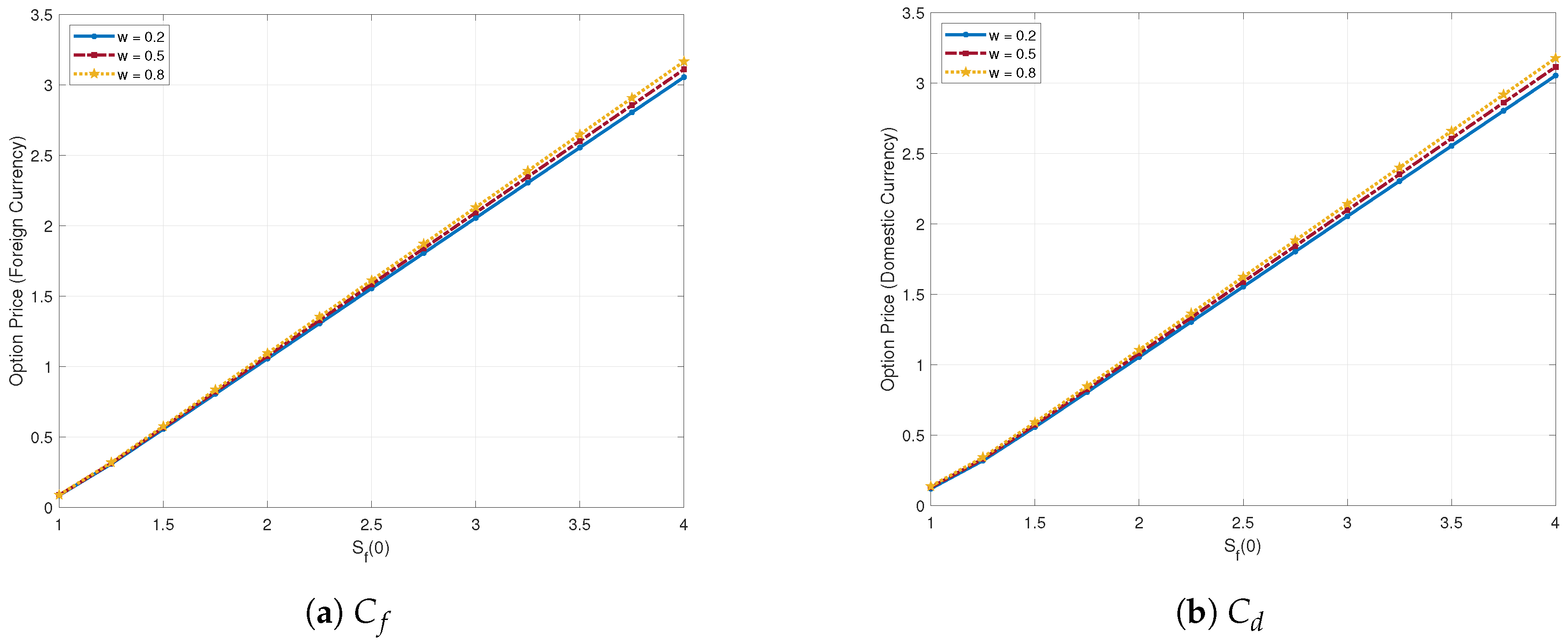
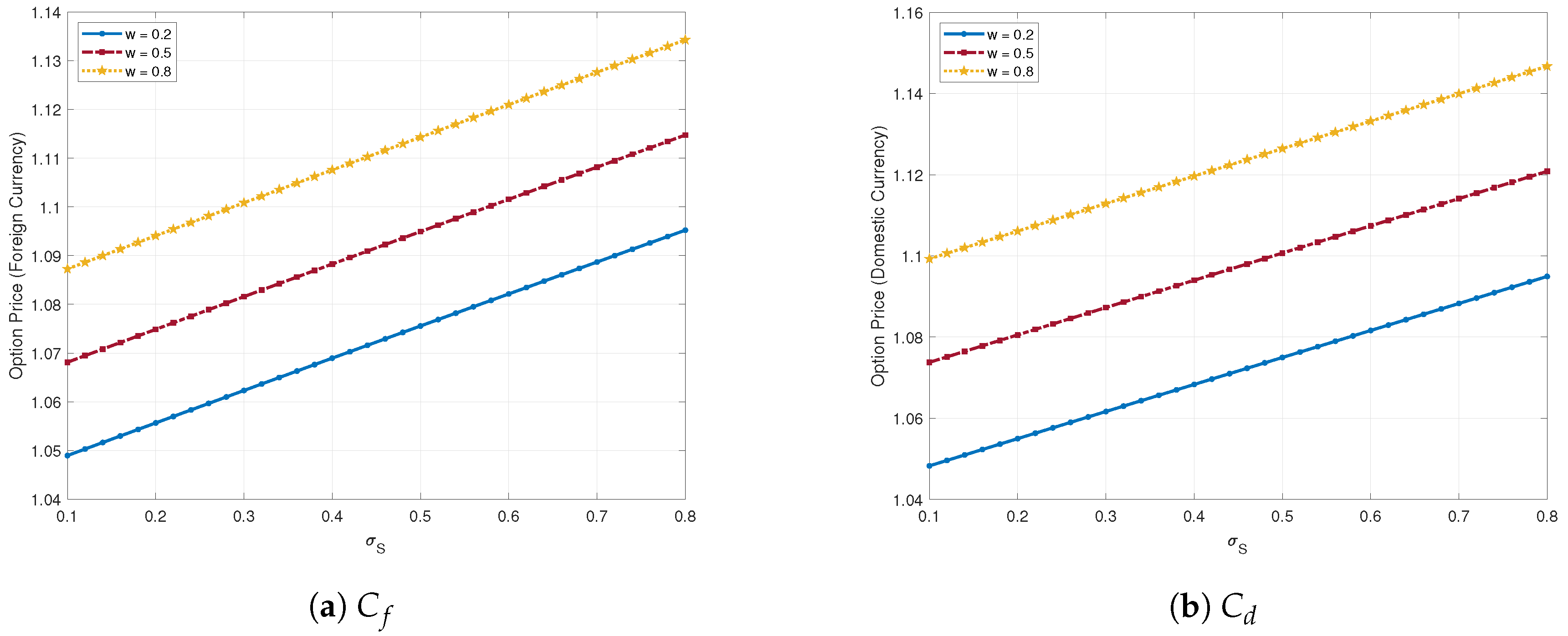
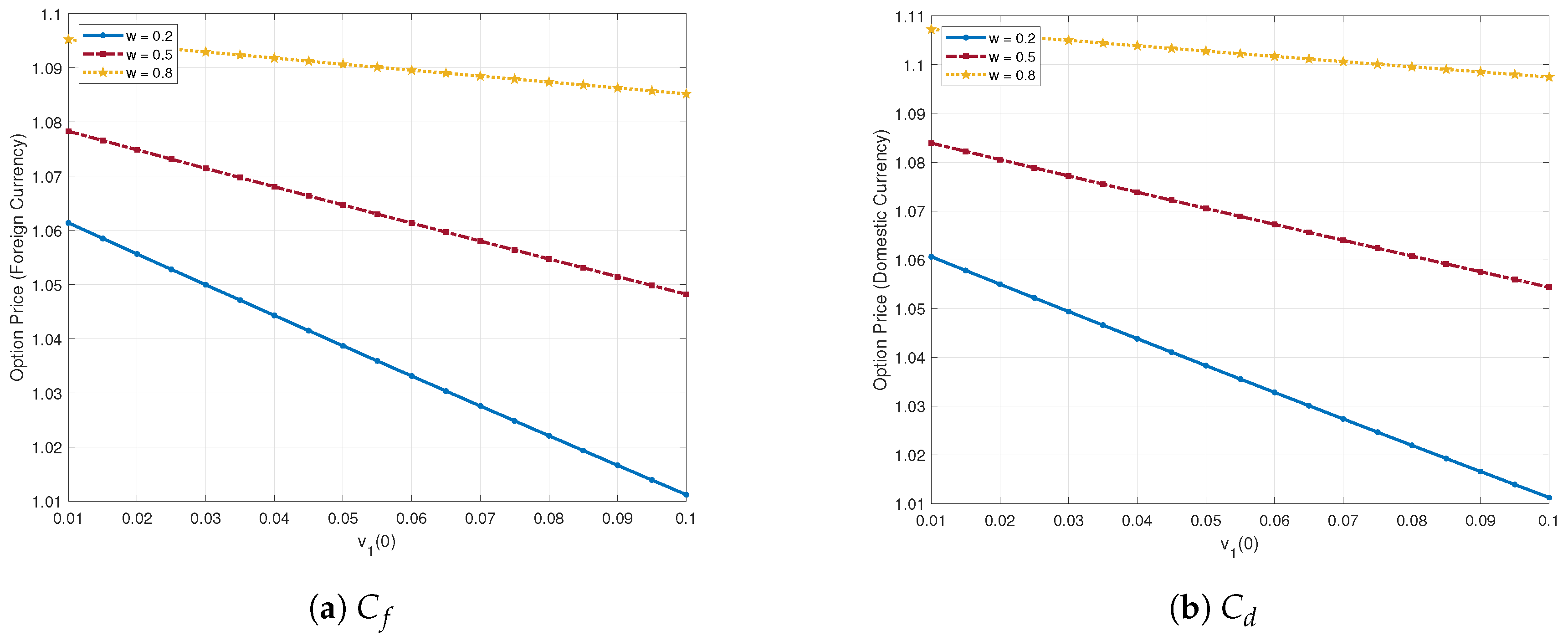
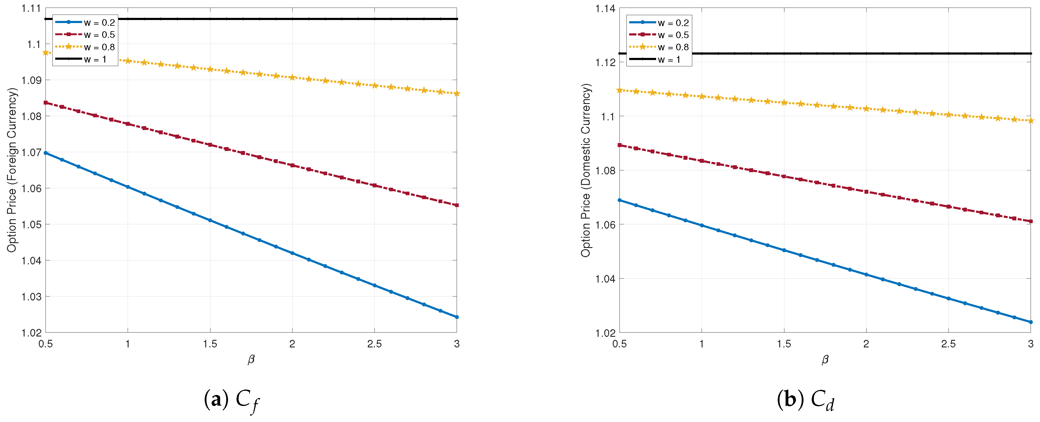
4. Numerical Examples

This section includes numerical examples demonstrating how the credit risk of the option issuer affects the prices of options and their sensitivity to significant parameters. The numerical examples present the prices of vulnerable foreign equity call struck in domestic currency and vulnerable foreign equity call struck in foreign currency. Obviously, both options have similar payoff functions, and thus we can find similar movements through experiments.

Table 1. Parameter values in the base case.

Parameter	Value	Parameter	Value
T	1	$r_f$	0.06
$S_f\left(0\right)$	2	$r_d$	0.05
$F\left(0\right)$	1	${\rho }_1$	−0.5
${\rho }_2$	0.2	$v_1\left(0\right)$	0.02
${\rho }_3$	0	$v_2\left(0\right)$	0.03
$a_1$	0.03	$v_3\left(0\right)$	0.06
$b_1$	1.1	${\gamma }_1$	0.3
$a_2$	0.02	${\gamma }_2$	0.2
$b_2$	2	${\gamma }_3$	0.2
$a_3$	0.02	$v\left(0\right)$	0.06
$b_3$	2	$\gamma$	0.01
a	0.02	$\beta$	1.25
b	2	w	0.4
$K_d$	1	$K_f$	1

indicates the parameter values for the base case, which are based on the works of Ma [8] and Wang [16].

Figure 1 illustrates the values of two kinds of vulnerable foreign equity options for three recovery rate scenarios under the proposed stochastic volatility model. Figure 1 shows that option prices grow logarithmically as the maturity T increases. This illustrates how option prices grow with maturity. Also, as expected, option prices with a high recovery rate w are higher than those with a low recovery rate w. Option prices with credit risk tend to decrease as w falls, which makes clear sense.

Figure 2 demonstrates how the initial stock price $S_f\left(0\right)$ affects option prices under different recovery rates. Both foreign and domestic currency options exhibit similar behavior, with prices increasing proportionally with $S_f\left(0\right)$. The effect of the recovery rate w is relatively small when the option is deep out of the money (low $S_f\left(0\right)$) but becomes greater as the option becomes in the money (high $S_f\left(0\right)$). This indicates that credit risk considerations are more significant for options with higher intrinsic value. Figure 3 illustrates the impact of stock price volatility ${\sigma }_S$ on option prices. As expected, higher volatility leads to higher option prices across all recovery rates, demonstrating the fundamental relationship between volatility and the option value. This relationship holds true for both foreign and domestic currency options, despite domestic currency options being slightly more sensitive to volatility changes.

Figure 4 shows how the initial volatility $v_1\left(0\right)$ affects option prices. The relationship is inverse; as the initial volatility increases, option prices decrease. This unexpected outcome can be explained by the interaction between credit risk and $v_1\left(0\right)$. This is because initial volatility $v_1\left(0\right)$ generates a high default intensity, which increases the credit risk of option issuers. The effect is significant for smaller recovery rates, implying that a high $v_1\left(0\right)$ increases credit risk issues. Figure 5 examines the relationship between the systematic risk parameter $\beta$ and option prices. As $\beta$ increases, option prices decrease across all recovery rates, with the effect being strongest for low recovery rates. This indicates how systematic risk has a direct impact on credit risk pricing, with higher systematic risk exposure resulting in larger price discounts. The effect is especially noticeable when w = 0.2, indicating that systemic risk issues are particularly significant when recovery rates are low. The case where w = 1 (no credit risk) served as an upper bound and showed no sensitivity to $\beta$, showing that $\beta$ exclusively influences prices through credit risk.

5. Concluding Remarks

This study presented and analyzed an extensive approach for pricing vulnerable foreign equity options which incorporates both stochastic volatility and credit risk using an intensity-based model. We derived explicit pricing formulas for two types of vulnerable foreign equity options with credit risk under a two-factor stochastic volatility model using the characteristic function and measure change techniques. The intensity-based model for determining credit risk covers both the systematic and idiosyncratic components of default intensity, providing a more realistic framework for pricing these options. In addition, we provided several numerical examples to demonstrate the impact of various parameters on option prices.

In this paper, we considered a two-factor stochastic volatility model for describing underlying assets. While the stochastic volatility model is a sufficient and appropriate model for real markets, jump diffusion models, regime-switching models, and others can be considered to extend the underlying asset models. Furthermore, to extend our results, it is also possible to consider models with liquidity risk, such as the recent work of Jeon and Kim [18]. In the future, these will be studied via the probabilistic approach with numerical methods.

References

1. Black, F.; Scholes, M. The pricing of options and corporate liabilities. J. Political Econ. 1973, 81, 637–654. [Google Scholar] [CrossRef]
2. Johnson, H.; Stulz, R. The pricing of options with default risk. J. Financ. 1987, 42, 267–280. [Google Scholar] [CrossRef]
3. Klein, P. Pricing Black-Scholes options with correlated credit risk. J. Bank. Financ. 1996, 20, 1211–1229. [Google Scholar] [CrossRef]
4. Jarrow, R.; Turnbull, S. Pricing options on financial securities subject to default risk. J. Financ. 1995, 50, 53–86. [Google Scholar] [CrossRef]
5. Lando, D. On Cox processes and credit risky securities. Rev. Deriv. Res. 1998, 2, 99–120. [Google Scholar] [CrossRef]
6. Kwok, Y.K.; Wong, H.Y. Currency-translated foreign equity options with path dependent features and their multi-asset extensions. Int. J. Theor. Appl. Financ. 2000, 3, 257–278. [Google Scholar] [CrossRef]
7. Huang, S.C.; Hung, M.W. Pricing foreign equity options under Lévy processes. J. Futur. Mark. Futur. Options Other Deriv. Prod. 2005, 25, 917–944. [Google Scholar] [CrossRef]
8. Ma, J. Pricing Foreign Equity Options with Stochastic Correlation and Volatility. Ann. Econ. Financ. 2009, 10, 303–327. [Google Scholar]
9. Sun, Q.; Xu, W. Pricing foreign equity option with stochastic volatility. Phys. A Stat. Mech. Its Appl. 2015, 437, 89–100. [Google Scholar] [CrossRef]
10. Fan, K.; Shen, Y.; Siu, T.K.; Wang, R. Pricing foreign equity options with regime-switching. Econ. Model. 2014, 37, 296–305. [Google Scholar] [CrossRef]
11. Xu, W.; Wu, C.; Li, H. Foreign equity option pricing under stochastic volatility model with double jumps. Econ. Model. 2011, 28, 1857–1863. [Google Scholar] [CrossRef]
12. Ma, Y.; Pan, D.; Shrestha, K.; Xu, W. Pricing and hedging foreign equity options under Hawkes jump–diffusion processes. Phys. A Stat. Mech. Its Appl. 2020, 537, 122645. [Google Scholar] [CrossRef]
13. Kim, D.; Yoon, J.H.; Kim, G. Closed-form pricing formula for foreign equity option with credit risk. Adv. Differ. Equ. 2021, 2021, 332. [Google Scholar] [CrossRef]
14. Kim, G. A Simplified Approach to the Pricing of Vulnerable Options with Two Underlying Assets in an Intensity-Based Model. Axioms 2023, 12, 1105. [Google Scholar] [CrossRef]
15. Fard, F.A. Analytical pricing of vulnerable options under a generalized jump–diffusion model. Insur. Math. Econ. 2015, 60, 19–28. [Google Scholar] [CrossRef]
16. Wang, X. Analytical valuation of vulnerable European and Asian options in intensity-based models. J. Comput. Appl. Math. 2021, 393, 113412. [Google Scholar] [CrossRef]
17. Shephard, N.G. From characteristic function to distribution function: A simple framework for the theory. Econom. Theory 1991, 7, 519–529. [Google Scholar] [CrossRef]
18. Jeon, J.; Kim, G. Analytically Pricing a Vulnerable Option under a Stochastic Liquidity Risk Model with Stochastic Volatility. Mathematics 2024, 12, 2642. [Google Scholar] [CrossRef]
Figure 1. The impact of the maturity T and recovery rate w on the option price.
Mathematics 13 00400 g001
Figure 2. The impact of the initial stock value S f ( 0 ) and recovery rate w on the option price.
Mathematics 13 00400 g002
Figure 3. The impact of the volatility σ S and recovery rate w on the option price.
Mathematics 13 00400 g003
Figure 4. The impact of the initial volatility v 1 ( 0 ) and recovery rate w on the option price.
Mathematics 13 00400 g004
Figure 5. The impact of the value of β and recovery rate w on the option price.
Mathematics 13 00400 g005