Abstract
Among the many methods of deep semi-supervised learning (DSSL), the holistic method combines ideas from other methods, such as consistency regularization and pseudo-labeling, with great success. This method typically introduces a threshold to utilize unlabeled data. If the highest predictive value from unlabeled data exceeds the threshold, the associated class is designated as the data’s pseudo-label. However, current methods utilize fixed or dynamic thresholds, disregarding the varying learning difficulties across categories in unbalanced datasets. To overcome these issues, in this paper, we first designed Cumulative Effective Labeling (CEL) to reflect a particular class’s learning difficulty. This approach differs from previous methods because it uses effective pseudo-labels and ground truth, collectively influencing the model’s capacity to acquire category knowledge. In addition, based on CEL, we propose a simple but effective way to compute the threshold, Self-adaptive Dynamic Threshold (SDT). It requires a single hyperparameter to adjust to various scenarios, eliminating the necessity for a unique threshold modification approach for each case. SDT utilizes a clever mapping function that can solve the problem of differential learning difficulty of various categories in an unbalanced image dataset that adversely affects dynamic thresholding. Finally, we propose a deep semi-supervised method with SDT called FldtMatch. Through theoretical analysis and extensive experiments, we have fully proven that FldtMatch can overcome the negative impact of unbalanced data. Regardless of the choice of the backbone network, our method achieves the best results on multiple datasets. The maximum improvement of the macro F1-Score metric is about 5.6% in DFUC2021 and 2.2% in ISIC2018.
MSC:
68T07
1. Introduction
Deep learning (DL) [1,2] is revolutionizing the way decisions are made across industries and is used in a wide range of fields, including natural language processing, medical and healthcare applications, and object recognition. Some models, such as Convolutional Neural Networks (CNNs) [3], Generative Adversarial Networks (GANs) [4], Recurrent Neural Networks (RNNs) [5], and Auto-Encoders [6], have been used frequently.
Convolutional Neural Networks are a rapidly growing and popular model structure for deep learning. It allows multi-layer computational models to extract higher-level features from raw inputs progressively. It has excellent performance in large-scale image processing and has a broad base of applications in areas such as autonomous driving systems [7], agriculture [8], and medical imaging [9,10]. For instance, autonomous driving systems leverage CNNs to interpret complex visual data in real time, ensuring safe and efficient navigation. Moreover, intelligent medicine applications utilize CNNs for medical image analysis, disease diagnosis, and personalized treatment plans. The continuous evolution and refinement of CNNs will undoubtedly lead to more sophisticated and innovative applications in the future, further integrating and enriching our daily lives.
However, its success heavily depends on having access to large-scale labeled data. When there is not enough labeled data available, the performance of deep networks decreases significantly [11]. In real-world scenarios, obtaining labeled data is expensive and sometimes impossible for nonspecialists, as with medical images.
Semi-supervised learning (SSL) [12] addresses this issue by employing a limited quantity of labeled training data in conjunction with a substantial amount of unlabeled data for training models. Adopting this approach can significantly lessen the labor of labeling data and swiftly enhance the network’s efficiency. In the recent past, deep semi-supervised learning has entered into a very interesting research problem, namely open-world [13]. Traditional learning methods were designed for a closed-world setting. However, the real world is inherently open and dynamic, so previously unseen classes may appear in test data or during model deployment [14]. As deep learning rapidly advances, applying deep semi-supervised learning (DSSL) [15] is suggested for fields challenging and expensive with data labeling, particularly in medical images. DSSL is a method that combines semi-supervised learning with deep learning models as the backbone network. It can be classified into five categories (i.e., pseudo-labeling, consistency regularization, generative methods [16,17], graph-based methods [18,19], and hybrid methods [20]).
The combination of consistency regularization and pseudo-labeling belongs to holistic/hybrid methods [21,22,23], a trend in SSL. Consistency regularization is founded on the principle that perturbed data output should remain consistent with its original output. Pseudo-labeling [24,25] is a prevalent technique in semi-supervised learning. The basic idea is that models trained using labeled data should produce similar predictions or identical pseudo-labels for the same unlabeled data. These pseudo-labels are used as additional instances to train the model. Different pseudo-label selection methods will lead to model performance variations, negatively affecting model performance if not implemented properly [26,27].
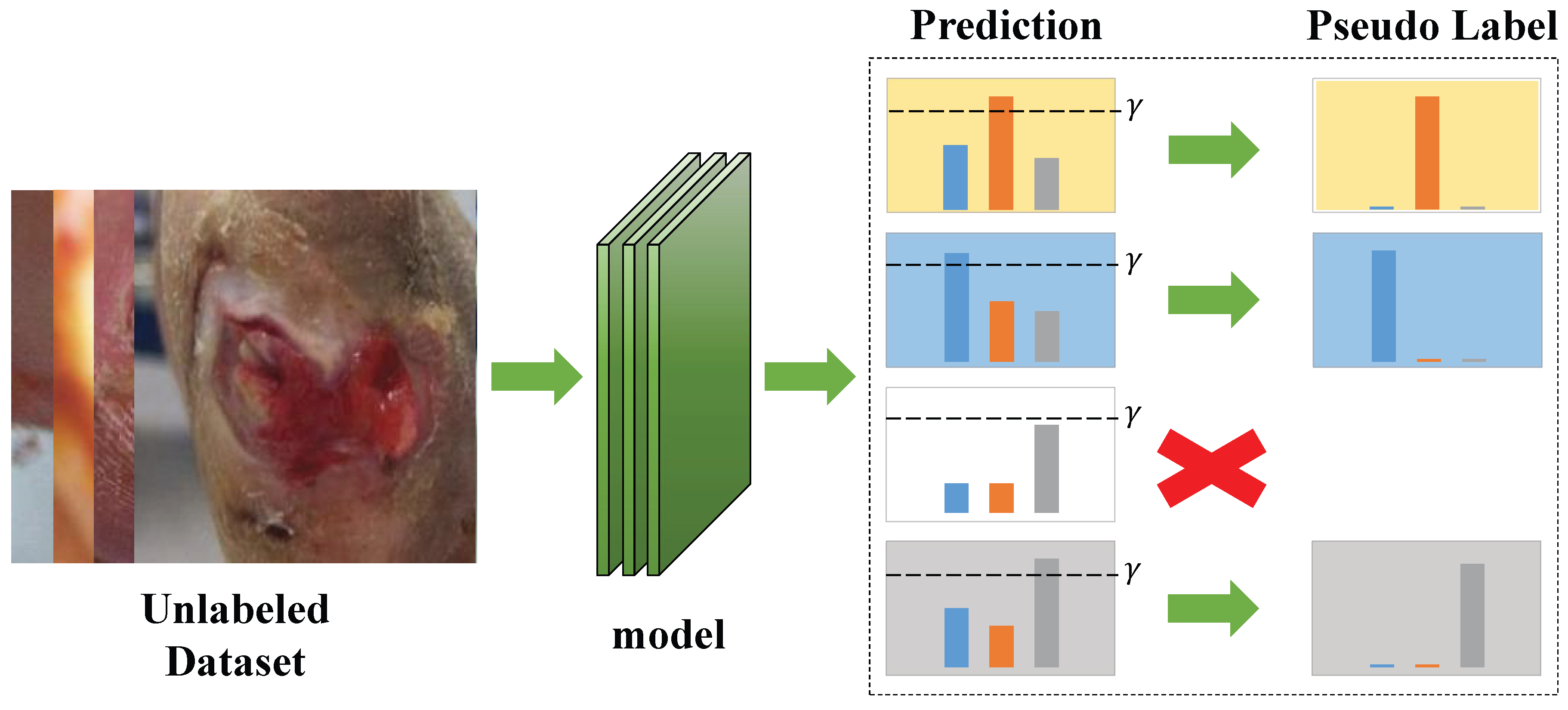
FixMatch [22], a holistic method, generates labels using consistency regularization and pseudo-labeling. Inspired by UDA [28] and ReMixMatch [21], FixMatch uses RandAugment [29] for strong augmentation to produce severely distorted versions of a given unlabeled image. Pseudo-labels are generated based on weakly augmented unlabeled images (e.g., enhanced using only flipped and shifted data). They will calculate the loss with the corresponding strong augmentation image prediction results. It is vital that FixMatch typically uses a fixed threshold to divide the classes obtained from model training of unlabeled data into two clusters, credible and noncredible. As shown in Figure 1, if the maximum prediction of unlabeled data exceeds , the corresponding class can be used as a pseudo-label to optimize the model. Otherwise, the unlabeled data has no pseudo-label.

Figure 1.
The unlabeled images are entered into the model to obtain the prediction results. Each bar chart shows the prediction results for different images.The individual class probabilities for an image are represented using different colors. Compare the maximum prediction to a fixed threshold, . If the prediction exceeds , the class associated with the maximum prediction is kept as a pseudo-label.
FlexMatch [30] argues that this high and fixed threshold can cause the model to under-consider the training difficulty of different categories, resulting in poorer results. Specific metrics can subtly indicate learning difficulty, but this requires partitioning the validation set, which is costly for medical data with limited labeling. Therefore, FlexMatch proposes a curriculum learning method, Curriculum Pseudo Labeling. They dynamically adjusted the threshold of each category during the training process without introducing additional parameters or computation. However, FlexMatch uses dynamic thresholding, adjusting the threshold for each class based on the number of unlabeled samples entering the model training. This approach only works when the number of images in each category is balanced. If the number of images varies greatly between classes, the threshold for the class with the smaller number is usually lower. The model is then prone to learning knowledge with lower confidence, reducing its classification accuracy.
Real datasets in many domains suffer from category imbalance. This affects the robustness of the model. Faced with such problems, researchers have proposed methods that use resampling (oversampling or undersampling) at the data level. For example, Lin, T.Y. et al. [31] proposes a novel undersampling method that offers significant advantages over other state-of-the-art methods on multiple publicly available datasets. However, resampling can be counterproductive [32]. In medical datasets, it is normal to have fewer cases at risk than in other data. Forced balancing can lead to models that may not be suitable for real-world applications. At the algorithmic level, some approaches modify the predictions of the underlying classifiers based on the frequency of each category, and others propose a new loss function that allows neural networks to handle unbalanced data streams online [33,34]. However, this requires a priori knowledge and does not consider avoiding the imbalance problem of deep semi-supervised learning.
In this paper, we design Cumulative Effective Labeling (CEL) to evaluate learning difficulty using ground truth and effective pseudo-labels. CEL contends that the greater the number of learning instances for a category, the easier it becomes for the model to grasp that category. It counts the ground truth and highly reliable pseudo-labels of each iteration to determine each class’s learning difficulty, which is used to calculate the threshold for each class in the next iteration. Additionally, we propose a way to calculate the threshold of each class with CEL, namely Self-adaptive Dynamic Threshold (SDT). SDT utilizes a hyperparameter and a clever mapping function to allow thresholds to adapt during learning. It follows the idea of having a high threshold when the learning difficulty is low and a low threshold when it is high. This approach helps prevent the model from acquiring incorrect knowledge and encourages it to learn efficiently from more data.
Our method, FldtMatch, combines SDT with a hybrid method and has demonstrated remarkable performance. It achieved superior results on the DFUC2021 and ISIC2018 datasets compared with other semi-supervised methods, regardless of the backbone network used. When using EfficientNet [35] as the backbone network on the DFUC2021 dataset, our method obtains a macro F1-Score of 60.25%, which exceeds FlexMatch, a well-known competitor in the field by about 5.6%. On the ISIC2018 dataset, our method outperforms other dynamic threshold adjustment strategies by a maximum of 2.2%.
In summary, this paper makes the following three contributions:
- We designed the Cumulative Effective Labeling (CEL) to better assess each category’s learning difficulty. CEL will serve in ensuing dynamic threshold calculation and learning model knowledge.
- We propose a Self-adaptive Dynamic Threshold (SDT) that can adapt to different situations by introducing only one hyperparameter. An innovative mapping function efficiently computes thresholds for a category under unbalanced datasets, significantly enhancing the model performance.
- SDT combined with a hybrid method for deep semi-supervised learning, named FldtMatch. Compared with other threshold adjustment methods, FldtMatch achieves the best results on multiple datasets, and even some of the training results are significantly higher than others.
2. Background
2.1. Convolutional Neural Networks
Since the introduction of AlexNet [36] in 2012, CNNs have undergone rapid advancements and evolution. VGGNet [37], building upon the foundation laid by AlexNet, significantly increased the depth of the model. However, this enhancement also introduced the challenge of gradient vanishing, a common issue in deep neural networks where gradients become exceedingly small, hindering training. To address this problem, ResNet [38] introduced the residual structure, a groundbreaking innovation that allowed gradients to flow more freely through the network. This residual connection, or “skip connection”, mitigates the gradient vanishing issue, thus enabling the training of much deeper networks. Due to its effectiveness, ResNet has become a classical model widely used in various application domains.
DenseNet [39] adopted a different approach to enhance network performance. By concatenating feature maps from all preceding layers, DenseNet encouraged feature reuse and uniquely mitigated the vanishing gradient problem. This approach allowed DenseNet to perform better than ResNet, with fewer parameters and computational costs. Despite these advancements, more explicit guidance on why specific depths and widths were chosen for these networks remained needed. Network dimensions such as width, depth, and resolution were traditionally scaled arbitrarily, often based on intuition or trial and error.
In 2020, Mingxing Tan and colleagues [35] proposed a novel approach to scaling network dimensions. Instead of arbitrarily scaling these dimensions, they introduced a simple and efficient composite coefficient to scale the model size uniformly. Through a series of experiments, they derived a family of smaller and faster models known as EfficientNets [35]. These models achieved state-of-the-art classification results on multiple datasets, demonstrating the effectiveness of their scaling method. EfficientNet represents a significant breakthrough in network architecture design, providing a systematic approach to scaling network dimensions. This innovation improves model performance and optimizes computational efficiency, making deep learning models more accessible and practical for real-world applications.
From VGGNet to EfficientNet, numerous researchers have applied them to the unbalanced medical image classification problem [40,41]. The outcomes of their efforts indicate that EfficientNet and DenseNet demonstrate superior performance in medical image classification compared with other network structures. Additionally, the BiT (Big Transfer) model [42], which builds upon the ResNeXt [43] architecture and leverages a significant amount of transfer learning from natural images, has also proven to be highly effective in the context of image classification. This model’s success further underscores the potential of transfer learning in unbalanced imaging tasks.
CNNs have emerged as one of the most iconic and pivotal neural networks in deep learning. These proven network structures are poised to become integral components of deep semi-supervised learning methods. Combining SSL with these advanced network architectures results in more accurate, efficient, and reliable diagnostic tools that ultimately help improve patient outcomes.
2.2. Semi-Supervised Learning
The loss function for semi-supervised learning is crucial. An accurately configured loss function enables the model to acquire knowledge of labeled and unlabeled data, particularly when labeled data is scarce. In semi-supervised learning, the loss typically comprises two elements: the supervised loss in labeled data () and the unsupervised loss in unlabeled data (). By merging these two elements using a weighting factor , the total loss is as follows:
The supervised loss, , is usually expressed as Equation (2), a computation based on the labeled data intended to improve the accuracy of the model’s predictions for these particular data points.
where M represents the number of labeled samples, is the m-th labeled sample, is the one-hot encoding ground truth of sample , is the probability of a sample generated by the model, and is the cross-entropy loss function. is identical to the loss function used in conventional supervised learning methods, frequently using cross-entropy loss to assess the variance between the model’s forecasts and actual labels. A smaller calculation implies comparable forecasts. The formula below defines the cross-entropy loss.
where C is the number of classes, is the predicted probability that the sample is of class i, y is the one-hot encoding of a sample’s ground truth, and holds the coding of this sample for category i. The coding will only be 0 or 1. 1 means that the sample is class i and 0 is not.
The unsupervised loss is computed on unlabeled data, aiming to encourage the model to make reasonable predictions for these data points. The of the holistic method, which combines the ideas of pseudo-labeling and consistency regularization, is as follows:
where N is the number of unlabeled images, is the indicator function that outputs 1 when the input is True and 0 when the input is False, is a strong augmentation function instead of a weak augmentation , is the n-th unlabeled sample, is a fixed threshold that screens for pseudo-labeling and is a pseudo-label. When calculating cross-entropy loss, is converted to one-hot encoding.
Equation (4) uses a fixed threshold . In image recognition tasks, the learning difficulty varies significantly across categories, often due to factors such as the number and complexity of available images. This discrepancy is particularly evident in domains such as medical imaging, where images of pathology at different stages may exhibit similar features as the disease progresses, making it difficult for models to distinguish between them. Moreover, relatively few high-risk cases lead to a scarcity of labeled images in these categories, which poses a significant challenge to machine learning models as they need to rely on a sufficient number of labeled examples to learn effective representations.
Given these challenges, applying a uniform threshold for image recognition tasks is often inappropriate. A fixed threshold represents a consistent difficulty in learning for the given category. Excessively high thresholds may exclude many unlabeled images from model training, hindering the model’s capacity to learn from varied data and effectively identify high-risk cases. Establishing a lower threshold can also lead to the acquisition of inaccurate knowledge. Both lead to a vicious cycle of performance degradation.
A dynamic threshold adjustment strategy adaptively generates thresholds for each category, which is conducive to utilizing unlabeled data and improving model performance. The general dynamic threshold calculation formula is as follows:
where is the dynamic threshold of class c and is the learning difficulty of class c at time step t. , the closer to 1, the easier it is to learn. The simple idea is to replace with the correctness of the validation set for each class. However, this requires additional validation sets and computations. Methods not requiring additional data and computation are more welcome in practical applications.
3. Method
FlexMatch draws inspiration from Curriculum Labeling (CL) [44] and introduces Curriculum Pseudo Labeling (CPL). CPL collects and keeps records of highly reliable predictions of model-generated unlabeled data. It then carefully calculated the frequency of each of these highly reliable predictions using the following formula:
where is the number of samples judged to be in category c with a probability capable of exceeding a threshold at time step t. is the prediction of the weak augmentation . is a pseudo-label for weak augmentation .
This counting mechanism helps us understand the distribution of different categories in the unlabeled dataset, which can guide subsequent learning strategies or refine the model’s predictions. The advantage of this statistical pseudo-labeling is that it does not require much additional computational work and maintains data processing efficiency. At the same time, the maximum predictive values of the counted samples must exceed predefined thresholds to ensure that frequent changes in categories during model instability do not adversely affect the calculation of dynamic thresholds. Determine the learning difficulty for each category, i.e., Equation (7).
where is from Equation (6).
Instead of using directly as in Equation (5), FlexMatch introduces the mapping function to compute the dynamic threshold as follows:
The mapping function effectively regulates the threshold change rate, setting a minimum threshold to prevent erroneous knowledge from being learned. FlexMatch offers three methods for calculating the threshold for each class: (1) concave: , (2) linear: , (3) convex: , and x is [30].
However, these mapping functions do not accommodate the case of unbalanced datasets. The reason is that some t-moment class c’ pseudo-labeled counts, , are too low due to the small number of samples belonging to category c, and the dynamic threshold is also low after Equations (7) and (8). Even after the model stabilizes after a training period, is consistently in a very low state. A low threshold indicates that the model learns low-confidence predictions as pseudo-labels. In other words, the model will likely learn the wrong knowledge, leading to slower convergence. In Section 4.4.1, we show the problems with Flexmatch more visually.
3.1. Cumulative Effective Labeling
CPL only accounts for the number of high-confidence prediction results, as indicated in Equation (6). The learning difficulty in Equation (8) is determined using Equation (7), which ultimately affects both the loss function and the model’s training process. However, the ground truth can have a more direct effect on learning difficulty. Since model training depends on the data, a large volume of data in a specific category will naturally influence the model’s learning process.
When the distribution of labeled data is unbalanced, meaning that some classes have significantly more labeled examples than others, the model’s training process can become biased. This bias can negatively impact its ability to make accurate predictions on unlabeled data. In other words, this bias can affect the selection of pseudo-labels generated from the model’s predictions on unlabeled data. Therefore, when using pseudo-labels for further training or analysis, we must consider potential imbalances in the labeled data distribution.
We propose Cumulative Effective Labeling, which takes the highly credible pseudo-labels and ground truth for each category as our effective labels as Equation (9).
where is from Equation (6), M represents a labeled number, and is the ground truth of the m-th label. It is not one-hot coding since no cross-entropy loss calculation is required. We then calculated the learning difficulty through Equation (10).
where is from Equation (9).
In practice, we can use an array to store the high-confidence prediction results for all samples. It is important to note that, as indicated in Equation (9), only prediction results that exceed a fixed threshold are recorded. This approach ensures the validity of the learning difficulty and the subsequent pseudo-labels’ reliability.
3.2. Self-Adaptive Dynamic Threshold
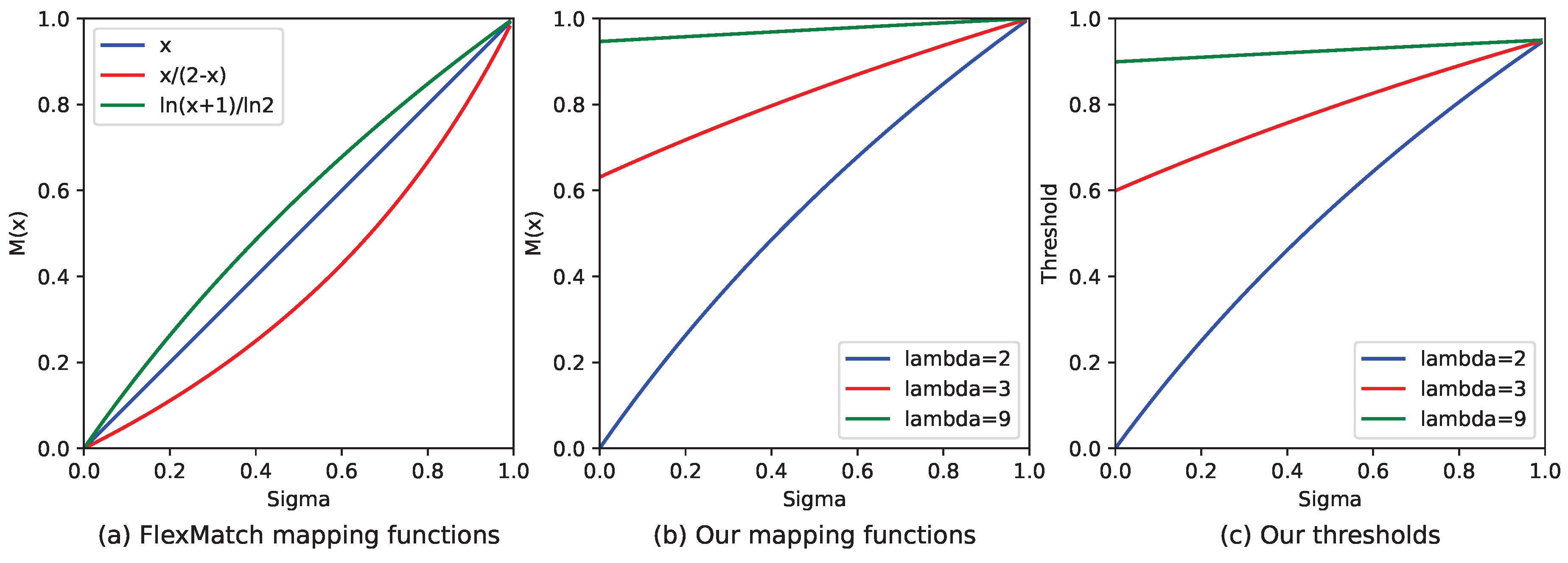
Figure 2a illustrates the linear, convex, and concave mapping functions. Our approach to dynamic threshold adjustment considers both the number of samples and changes in quantity. Categories with a large amount of training data have higher thresholds, and fluctuations in quantity have little impact on these thresholds, which remain stable. In contrast, when there is limited data, the thresholds start low. However, as the amount of data increases, the thresholds are raised rapidly, ensuring the model converges more quickly. As a result, the linear mapping function is unsuitable for our purposes.
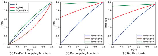
Figure 2.
(a) Shows three typical mapping functions: linear, convex, and concave. We can discover the changing pattern of the curve and choose the appropriate mapping function to adjust the threshold. (b) Is our mapping function, as shown in Equation (11), with different . (c) Represents the threshold case when applying the mapping function of (b).
When comparing the suitability of convex and concave functions for modifying thresholds, especially in unbalanced datasets, the concave function emerges as the more appropriate choice. Concave functions inherently possess characteristics that allow for more nuanced and gradual adjustments to thresholds, which is particularly beneficial when dealing with datasets where the distribution of classes is uneven.
To this end, we propose a simple yet effective dynamic threshold method, Self-adaptive Dynamic Threshold. The focus is on designing the mapping function as Equation (11).
where x is from CEL and is a hyperparameter.
Setting up specialized mapping functions for all datasets is not possible. SDT application spans numerous situations, necessitating only the incorporation of a hyperparameter . In Figure 2b, we present several typical examples of adjusting thresholds dynamically. The parameter influences these curves’ minimum value and steepness. Specifically, as the value of increases, the curve becomes smoother, leading to a gentler change in the threshold. At the same time, the SDT ensures a lower threshold limit, preventing the threshold from being too low in categories with a limited number of samples. This threshold adjustment method is sensitive and stable, mainly when working with unbalanced datasets.
Researchers can flexibly modify the parameter according to the specific dataset and experimental situation. When the number of images in each category is relatively balanced, can be set to a smaller value. In this way, the model can accelerate convergence. Conversely, if there is a significant imbalance in the number of instances per category, should be set to a relatively large value. In Section 4.4.3, we discuss ’s taking of values in more detail.
This approach prevents the threshold from becoming too low, as illustrated in Figure 2c, which could lead to the model incorporating erroneous information. Doing so helps mitigate the model’s bias towards categories with a more significant number of instances.
Such a strategic modification of based on the observed class distribution goes a considerable distance toward alleviating the problems caused by quantitative imbalances in the dataset. It fosters a more equitable treatment of all classes, enhancing the model’s overall performance and robustness in making accurate predictions across the entire spectrum of classes present. Based on Equation (11), our SDT is calculated as shown below:
The loss function for unlabeled images at time step t is as Equation (13).
where denotes the number of unlabeled images entering the model training at moment t, and is from Equation (12). For any unlabeled sample , the maximum value of must exceed the corresponding category dynamic threshold . Only then can we consider the pseudo-label reliable enough to compute the loss of .
3.3. FldtMatch: DSSL with Self-Adaptive Dynamic Threshold
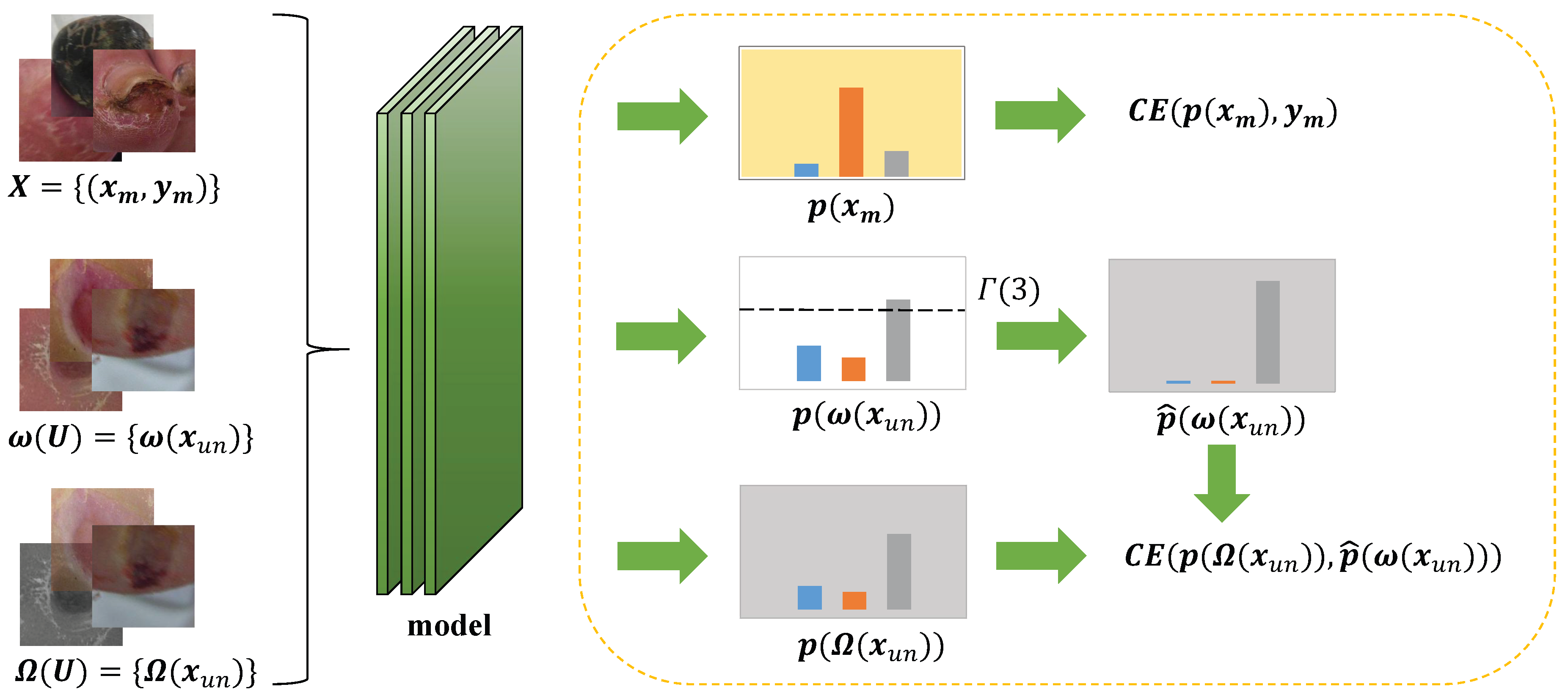
To fully realize the potential of SDT, it needs to be integrated with a specific semi-supervised approach. We introduce FldtMatch, a method that combines SSL with a holistic approach to develop a new deep semi-supervised learning technique. This holistic approach incorporates the concepts of consistency regularization and pseudo-labeling, which are briefly outlined in Section 1. This combination dynamically adjusts thresholds to promote more accurate and efficient learning from limited labeling data. To illustrate the model training process employing FldtMatch, we provide a graphical representation in Figure 3 and a detailed algorithmic description in Algorithm 1.
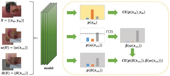
Figure 3.
FldtMatch: DSSL with Self-adaptive Dynamic Threshold. The yellow dashed box on the right takes a labeled image and an unlabeled image as an example. The model can use any Convolutional Neural Network as a backbone network.
Suppose we have a training set , where X represents the labeled dataset and U represents the unlabeled dataset. Each tuple in X comprises image and image label , which is the ground truth. In U, there are only unlabeled images, such as , and no ground truth.
During any iteration t, we will use Equations (9)–(12) to compute the thresholds for each category, e.g., of Figure 3 represents the third class of dynamic thresholds, and Algorithm 1 shows the computation of how it is obtained. Subsequently, weak augmentation and strong augmentation are applied to each unlabeled image of a batch to obtain weak augmentation images and strong augmentation images, respectively. Strong augmentation transforms the data more drastically, while weak enhancement applies milder changes. They aim to preserve the basic features of the image while introducing some variability. Weak and strong augmentation images, along with labeled images of the same batch, are used in model training to obtain their corresponding results.
The predictions for the labeled images are directly compared with their ground truth annotations to compute the supervised loss as following Equation (14). This loss quantifies the discrepancy between the model’s predictions and the actual labels, providing a direct measure of the model’s performance on the labeled portion of the dataset.
where denotes labeled image number at iteration t.
For the unlabeled data, pseudo-labels are first generated based on dynamic threshold and the model’s predictions on the weak augmentation images. These pseudo-labels serve as temporary labels for the unlabeled data, reflecting the model’s current understanding of the data distribution. Subsequently, these pseudo-labels are compared with the model’s predictions on the corresponding strong augmentation images to calculate the unsupervised loss as Equation (13). This loss measures the consistency between the model’s predictions across different augmentations of the same image, encouraging the model to produce robust and consistent predictions even when faced with variations in the input data. Finally, we combine and for the optimization model in the same way as in Equation (1). is a hyperparameter, which we set to 1 in this paper.
The initialization phase has a time complexity of , where C is the class number, and N is the unlabeled image number. Next, as the model begins training, it is necessary to compute CEL for each category. This can be accomplished in a single traversal, resulting in a time complexity of , in which M is the labeled image number. Finally, calculating the learning difficulty and dynamic threshold has a time complexity of . Since both CEL and SDT need to be computed in each iteration, the method’s time complexity is , in which T is the iteration number. Given that C is much less than , this simplifies to .
| Algorithm 1 FldtMatch: DSSL with Self-adaptive Dynamic Threshold |
|
4. Experiments
4.1. Environment and Metric
In this paper, we conducted our experiments and analyses using an RTX 4090 graphics card with 24 GB of dedicated memory, the Python programming language at version 3.12.4, and the Torch library (specifically version 2.2.2).
The primary performance evaluation metric utilized in this context is the macro F1-Score, a comprehensive measure that balances precision and recall. The formulas are as follows:
where TP is True Positive, FP is False Positive, FN is False Negative, and C is the number of classes.
First, for each class within the dataset, precision as shown in Equation (15) (the ratio of correctly predicted positive observations to the total predicted positives) and recall, as shown in Equation (16) (the ratio of correctly predicted positive observations to all observations in the actual class) are computed separately. Second, the precision and recall values were used to calculate the F1-Score for each category, according to Equation (17). Finally, the macro F1-Score is obtained by averaging the F1-Scores of all classes as shown in Equation (18), providing an overall indication of the model’s performance across all classes, without being biased by the class distribution or the performance of any particular class. The macro F1-Score is a performance evaluation metric commonly used in machine learning, particularly in multi-class classification tasks.
In addition to the F1-Score, AUC (Area Under the Curve) can also evaluate models in conjunction with Recall and Precision. The macro AUC, which is the average of the AUCs of each category, can reliably assess the classifier’s performance, especially in the case of sample imbalance. AUC measures the area under the ROC (Receiver Operating Characteristic) curve. One of the ROC curve’s key advantages is its ability to remain stable even when the data distribution changes. The horizontal coordinate of the ROC curve is the False Positive Rate (FPR), and the vertical coordinate is the True Positive Rate (TPR). Their formulas are as follows:
4.2. Datasets
The datasets employed in this study are DFUC2021, cited in references [46,47], ISIC2018, referenced in [48,49], and CIFAR-10, referenced in [50]. Both datasets are designed for classification tasks and present unique challenges for machine learning models. Table 1 reflects the basic distribution of the three datasets.

Table 1.
A description of the different datasets when they are actually trained. Imbalance Ratio is a number that denotes the ratio between majority and minority classes. Class Populations refer only to the labeled images.
4.2.1. DFUC2021
The DFUC2021 dataset comprises a substantial collection of images, specifically 5955 labeled images, 3994 unlabeled images, and an additional 5734 unlabeled test images. These images are categorized into four distinct classes, each with a uniform resolution of 224 × 224 pixels. The classes include none, infection, both, and ischemia, reflecting various conditions related to diabetic foot ulcers.
Notably, the DFUC2021 dataset exhibits a significant imbalance in class distribution. Specifically, there are 2552 images labeled as none, 2555 images labeled as infection, 621 images labeled as both (indicating both infection and ischemia), and only 227 images labeled as ischemia. This imbalance, with a ratio of approximately 11:11:3:1, poses a challenge for machine learning models, as they must perform well in all classes despite the disparity in sample sizes.
4.2.2. ISIC2018
The ISIC2018 dataset is a 7-classification task with 10,015 labeled images and 1512 labeled test images, each 600 × 450 pixels in size. The ISIC2018 classification task includes seven types of diseases: actinic keratosis (AKIEC), basal cell carcinoma (BCC), benign keratosis (BKL), dermatofibroma (DF), melanoma (MEL), melanocytic nevus (NV), and vascular lesion (VASC). The number of categories for MEL, NV, BCC, AKIEC, BKL, DF, and VASC are 904, 6184, 483, 318, 981, 101, and 129, respectively. The dataset is also unbalanced. Owing to the scarcity of training resources, every image encompassing both training and testing phases was condensed to a resolution of 224 × 224 pixels.
The ISIC2018 dataset, unlike DFUC2021, does not inherently contain unlabeled images. Therefore, to facilitate semi-supervised learning, we manually divide a portion of its labeled images into an unlabeled set. Specifically, we allocate 40% of the labeled images from ISIC2018 to serve as unlabeled images, leaving the remaining 60% as labeled for training purposes. It is worth noting that dividing the dataset needs to ensure that the distribution of unlabeled and labeled data remains consistent. This step is vital to avoid introducing biases that could adversely affect the performance of the semi-supervised learning model.
4.2.3. CIFAR-10
CIFAR-10 is a dataset with 10 categories, namely airplane, automobile, bird, cat, deer, dog, frog, horse, ship, and truck. Each category has 6000 samples, each sample is a 32 × 32 pixel color image. These 60,000 samples are divided into 50,000 training samples and 10,000 test samples. In the experiment, the training samples for each category were reduced in order, i.e., 5000 for the first category, 4500 for the second category, 4000 for the third category, and so on. Additionally, 40% of the samples are designated as unlabeled data. As a result, the distribution of labeled and unlabeled data will be unbalanced.
4.3. Parameter Settings and Main Results
We carefully compare FldtMatch, as outlined in Algorithm 1, with other DSSL methods, specifically FixMatch and FlexMatch. FixMatch utilizes a fixed threshold throughout the training process, while FlexMatch employs a dynamic threshold that adjusts according to the model’s evolving state. FlexMatch uses Equation (8), where the mapping function is . Our approach is based on Equation (12). For DFUC2021 and ISIC2018, is set to 10. For CIFAR-10, is set to 2. To understand how to set the parameter effectively, we delve into a detailed analysis in Section 4.4.3.
Deep semi-supervised learning frameworks inherently require a robust model as the backbone network for both the training and prediction phases. Drawing on the previous research paper in [51] and the analysis of CNNs in Section 2.1, we deliberately chose to utilize EfficientNet and BiT as our backbone models. These architectures are renowned for their strong performance in various computer vision tasks and are well-suited to handle the complexities associated with semi-supervised learning scenarios.
We ensured a comprehensive evaluation of the experimental parameter settings by setting the number of epochs to 300. It allows the models sufficient time to converge and learn effectively from the labeled and unlabeled data. The parameter is 0.95. For the optimization algorithm, we opted for Stochastic Gradient Descent (SGD) with a momentum of 0.9, a configuration known for its stability and efficiency in training deep neural networks. The initial learning rate (lr) is 0.01, a common starting point that balances exploration and exploitation during training.
To further refine the learning process, we incorporated the CosineAnnealingWarmRestart method for learning rate decay. This technique periodically resets the learning rate to its initial value (in this paper, after every three epochs), followed by a cosine decay cycle. The lr change rate is 2, which controls the magnitude of the learning rate fluctuations during each cycle. This method provides a mechanism for the model to periodically escape local minima, thereby enhancing its ability to find a more optimal solution in the loss landscape.
Table 2, Table 3 and Table 4 show the classification results for DFUC2021 dataset, ISIC2018 dataset and CIFAR-10 dataset, respectively. All the numerical values are better when they are more extensive. Boldly emphasized values indicate the most favorable results achieved by a metric.
Table 2.
Evaluating various methods for adjusting thresholds on the DFUC2021 dataset.
Table 3.
Evaluating various methods for adjusting thresholds on the ISIC2018 dataset.
Table 4.
Evaluating various methods for adjusting thresholds on the CIFAR-10 dataset.
4.4. Analysis
In this subsection, we begin by analyzing the reasons behind the poor classification metrics of FlexMatch. Second, we compare the main results presented in Section 4.3 to demonstrate the robustness of FldtMatch when handling unbalanced datasets. Finally, we include additional experiments to provide insights into selecting the hyperparameter .
4.4.1. Why Does Flexmatch Give Poor Results?
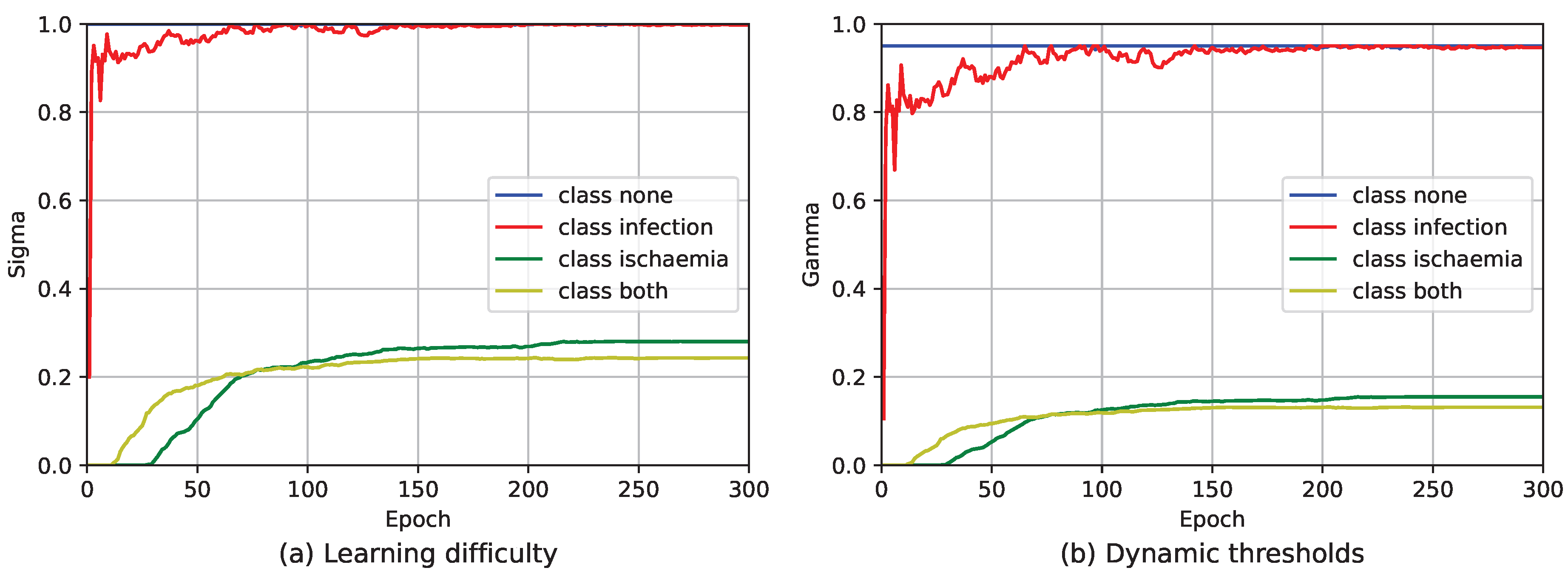
In Section 3, we briefly covered the issue of Flexmatch. Figure 4 shows the variation in learning difficulty and dynamic threshold for the FlexMatch method on the DFUC2021 dataset.
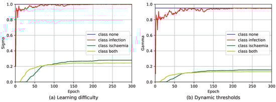
Figure 4.
The change in learning difficulty and dynamic thresholds throughout the model training period under the FlexMatch method. The mapping function is and .
From Figure 4a, we can see that class none has the highest , followed by class infection, while class ischemia and class both have of about 0.2. This is because the DFUC2021 dataset has fewer samples for class ischemia and class both, resulting in a lower corresponding to Equation (6). After Equation (7), i.e., the of each class is divided by the highest , the final effect is presented in Figure 4a. After the calculation of Equation (8), the dynamic thresholds for class none and class infection are high, while those for class ischemia and class both are low, as shown in Figure 4b.
Depending on the number of samples in the class, low dynamic thresholds persist. This allows some low predictions to generate pseudo-labels, perform loss calculations, and eventually be learned by the model. Take a sample s of a class both as an example, if the model predicts a result for ischemia, even if , Flexmatch will compute the pseudo-labeling for s, and ultimately compute the loss L, and the model learns that result. This is an unreasonably low predictive probability being learned by the model. This is also illustrated by the results on FlexMatch in Table 2, Table 3 and Table 4.
4.4.2. Analysis of Main Results
Regarding our primary metric, the macro F1-Score, as shown in Equations (17) and (18), our method, FldtMatch, consistently outperforms other methods across various datasets and models, demonstrating a significant improvement. It indicates that the SDT component is a crucial factor in the performance of FldtMatch.
The macro F1-Score for FldtMatch using EfficientNet-B3 showed a notable improvement over FlexMatch in DFUC2021, with an increase of approximately 5.6%. When using the BiT-M-R101x1 backbone network, our method improved by about 2.2% compared with FlexMatch in ISIC2018. In CIFAR-10, FldtMatch has a slight edge over FixMatch and FlexMatch regarding Macro F1-Score. We believe that this is a result of the nonsignificant inter-category imbalance in CIFAR-10. The imbalance in CIFAR-10 was artificially created by the experimenter, with some subjective effects. It is interesting to note that the BiT-M-R101x1 backbone generally outperforms the EfficientNet-B3 across all methods. This suggests that the BiT-M-R101x1 backbone might be more effective for this particular task on the CIFAR-10 dataset.
FixMatch under the BiT model obtains the best macro Recall in the ISIC2018, which we attribute to the fitness of the backbone network to the data distribution. FlexMatch consistently demonstrates the best performance regarding macro Recall in most cases, which is affected by how its threshold is determined. As shown in Figure 4, FlexMatch maintains a very low threshold for an extended period for categories with limited images. Lowering the threshold makes it easier to select pseudo-labels, allowing more positive examples to be incorporated into model training. This effectively reduces the false negatives (FNs) in Equation (16).
However, this approach leads to a decrease in macro Precision. Table 2 and Table 3 also show that the best macro Recall corresponds to the worst macro Precision. Since the training data heavily influence the model, the risk of a counterexample being incorrectly predicted as a positive example (false positives, FP, in Equation (15) also increases significantly. As a result, FlexMatch ultimately exhibits the lowest macro Precision, with a substantial about 8% gap compared with other methods.
As with the primary metric macro F1-Score, FldtMatch obtains the best results in macro AUC regardless of the dataset and backbone network. ACC (Accuracy) metric gauges how correctly the model categorizes data but could perform better in balanced datasets. This is because the model may exhibit bias by predominantly predicting the categories with the highest number of samples, which can inflate the accuracy value.
4.4.3. Analysis of Hyperparameter Selection
In Section 3.2, we mentioned the parameter settings, which can be tailored to accommodate various situations and exhibit high flexibility. However, despite this versatility, we recommend limiting the value of to the range of [2, 10] for optimal performance and stability. First, based on the fundamental characteristics of the logarithmic function, must be greater than 0. Moreover, cannot be set to 1 due to the specific mathematical properties and behaviors associated with this value in the context of our application.
Secondly, the mapping function must progressively increase in a predictable and controlled manner to guarantee that as the amount of learning increases, the threshold also becomes more elevated. This requirement necessitates that surpasses 1 to ensure a positive and increasing slope in the mapping function. It is crucial that initiate from a value of at least 2. This prevents the possibility of taking on negative values, which could result in a negative threshold and potentially lead to undefined or undesirable behaviors in the system.
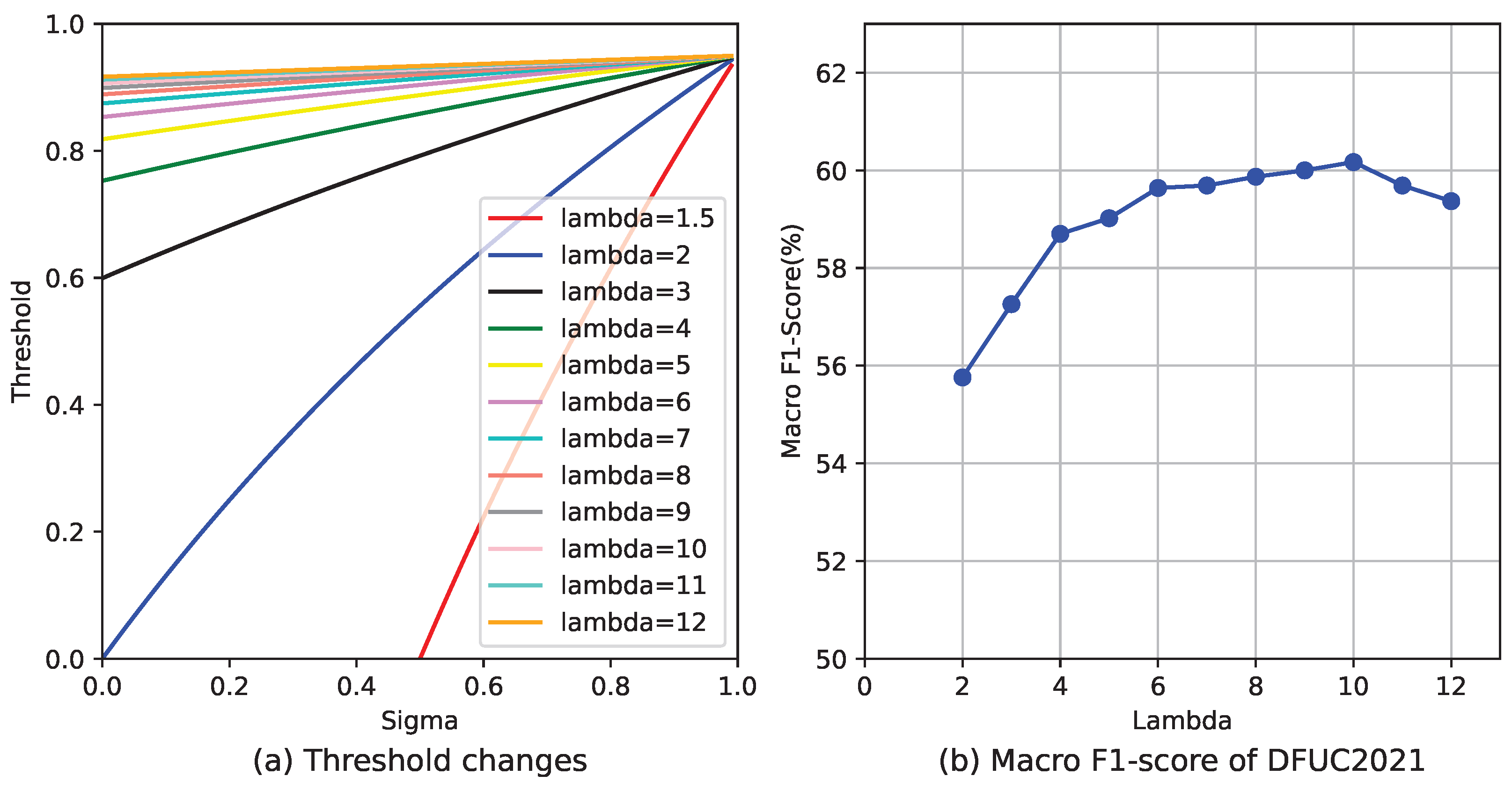
As illustrated in Figure 5a, adjusting to values above ten results in only minor and insignificant variations in the curve, indicating that further increases in beyond this point offer diminishing returns and may not be necessary or beneficial. Figure 5b illustrates macro F1-Score across various lambdas for the DFUC2021 dataset.
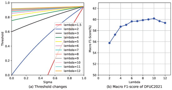
Figure 5.
(a) Shows more threshold curves under our mapping function with different . When is excessively high, there’s a slight variation in the thresholds regardless of the changes in . (b) Illustrates the macro F1-Score for DFUC2021 under varying values, with optimal outcomes attained at = 10.
Our meticulous experimental observations and analyses have found that the parameter can be effectively considered N in specific circumstances. These circumstances arise when the maximum multiple of the number between different categories is N, and this value N does not exceed 10. In other words, the maximum difference in quantity between any two categories in our dataset can be expressed as a multiple of N. Setting to N produces beneficial results when N ranges from 1 to 10. This finding suggests a potential link between data distribution and the optimal setting of the parameter. It can help us tailor our approach more precisely to the characteristics of a specific problem.
4.5. Testing Stability
We modified the dataset’s data volume to perform stability tests on FldtMatch, as shown in Table 5. The quantity change is divided into two cases: (1) Percentage: modifying the proportion of unlabeled data; (2) Decrease: modifying the number of labeled samples. The experiments in this section are mainly conducted on the ISIC2018 dataset, using BiT-M-R101x1 as the backbone network. The quantity change is divided into two cases: modifying the proportion of unlabeled data and the proportion of overall samples. The experiments in this section are mainly conducted on the ISIC2018 dataset, using BiT-M-R101x1 as the backbone network.
Table 5.
Testing Stability in the ISIC2018 dataset. All results in the table are Macro F1-Score. “Percentage” means unlabeled as a percentage of overall.
Compared with the macro F1-Score of 67.09% in Table 3, the result for Percentage = 0.5 decreases by 0.37%. This suggests that classifying more labeled as unlabeled images did not affect the model’s results much. Gradually increasing the proportion of unlabeled also resulted in a steady decrease in the metric of 0.3–0.5%.
Reducing the number of labeled images has a more severe impact on the model than changing the unlabeled percentage. The categorization metrics drop significantly due to much less useful data information. Reducing the number of labeled images by 10% decreases the model’s classification metrics by approximately 3%.
4.6. Ablation Experiment on CEL
Before this subsection, we have experimentally analyzed to determine the effectiveness of the SDT method for model performance improvement. The learning difficulty as shown in Equations (9) and (10) is used to help SDT compute dynamic thresholds for various categories. We propose CEL to improve CPL on calculation. We design ablation experiments to demonstrate the effectiveness of CEL, as shown in Table 6.
Table 6.
Ablation experiment on CEL in the DFUC2021 dataset. Boldly emphasized values indicate the most favorable results achieved by a metric.
We applied SDT based on the overall method in Figure 3 but changed the calculation of learning difficulty by replacing CPL with CEL. The higher macro F1-Score metrics obtained using CEL compared with CPL demonstrate its importance. We need to count high-confidence pseudo-labeling and ground truth to calculate the learning difficulty.
5. Conclusions and Future Work
Holistic methods that utilize consistency regularization and pseudo-labeling in deep semi-supervised learning have shown promising results. Typically, these methods require thresholds to select pseudo-labels. However, it has been observed that existing methods—whether they use fixed or dynamic thresholds—are often ineffective when dealing with unbalanced data. This paper introduces Cumulative Effective Labeling (CEL) to better reflect actual learning difficulty. Next, we propose a novel approach called Self-adaptive Dynamic Threshold (SDT) to address the issues arising from the uneven distribution of images across different categories in the unlabeled dataset. SDT is simple and effective, requiring only a single hyperparameter to accommodate many scenarios. It provides real-time, appropriate thresholds for each category, unlike fixed thresholds that frequently overlook the complexities and dynamics of real-world datasets. Moreover, our SDT approach stands out from other dynamic threshold adjustment methods by tackling a crucial challenge: the threshold often needs to be raised sufficiently for categories with limited images. To demonstrate the effectiveness of our proposed method, FldtMatch, we conducted extensive experiments on three benchmark datasets: DFUC2021, ISIC2018 and CIFAR-10. Our experiments show that the CEL method is effective, while the SDT method exhibited robust performance, outperforming traditional fixed threshold methods and other dynamic threshold adjustment strategies. Looking ahead, we plan to integrate our SDT method with a diffusion model to enhance the clarity and quality of medical imagery.
Author Contributions
Conceptualization, X.W. and K.L.; methodology, X.W. and K.L.; software, X.W.; validation, X.W. and J.X. (Jingjing Xu); formal analysis, X.W. and K.L.; investigation, X.W. and J.X. (Jingjing Xu); resources, X.W. and J.X. (Jingjing Xu); data curation, X.W. and J.X. (Jingjing Xu); writing—original draft preparation, X.W.; writing—review and editing, K.L. and J.Y.; visualization, X.W.; supervision, K.L. and J.Y.; project administration, J.X. (Jian Xiong); funding acquisition, J.X. (Jian Xiong). All authors have read and agreed to the published version of the manuscript.
Funding
This research was supported by the Guangdong Provincial Key Discipline Research Capacity Improvement Project on ‘Research on the Application of Artificial Intelligence Based on Medical Imaging Big Data’, project number: 2022ZDJS152. And this research was supported by the Guangdong Provincial Key Discipline Research Capacity Improvement Project on ‘Statistical Inference of the Subgroup Average Treatment Effect’, project number: 2024ZDJS132.
Data Availability Statement
We open source our code at https://github.com/Altercg/Self-adaptive-Dynamic-Threshold (accessed on 21 January 2025). DFUC2021 dataset needs to be obtained from the official application. Detailed links are as follows: https://dfu-challenge.github.io/dfuc2021.html. We declare that the ISIC2018 dataset associated with this project is officially fully open-source and available to the public.
Conflicts of Interest
The authors declare no conflicts of interest.
Correction Statement
This article has been republished with a minor correction to the Funding statement. This change does not affect the scientific content of the article.
References
- Sarker, I.H. Deep Learning: A Comprehensive Overview on Techniques, Taxonomy, Applications and Research Directions. SN Comput. Sci. 2021, 2, 420. [Google Scholar] [CrossRef] [PubMed]
- Ahmed, S.F.; Alam, M.S.B.; Hassan, M.; Rozbu, M.R.; Ishtiak, T.; Rafa, N.; Mofijur, M.; Shawkat Ali, A.B.M.; Gandomi, A.H. Deep learning modelling techniques: Current progress, applications, advantages, and challenges. Artif. Intell. Rev. 2023, 56, 13521–13617. [Google Scholar] [CrossRef]
- Habib, G.; Qureshi, S. Optimization and acceleration of convolutional neural networks: A survey. J. King Saud Univ.-Comput. Inf. Sci. 2022, 34, 4244–4268. [Google Scholar] [CrossRef]
- Lim, W.; Yong, K.S.C.; Lau, B.T.; Tan, C.C.L. Future of generative adversarial networks (GAN) for anomaly detection in network security: A review. Comput. Secur. 2024, 139, 103733. [Google Scholar] [CrossRef]
- Quradaa, F.H.; Shahzad, S.; Almoqbily, R.S. A systematic literature review on the applications of recurrent neural networks in code clone research. PLoS ONE 2024, 19, e0296858. [Google Scholar] [CrossRef]
- Chen, S.; Guo, W. Auto-encoders in deep learning—A review with new perspectives. Mathematics 2023, 11, 1777. [Google Scholar] [CrossRef]
- Turay, T.; Vladimirova, T. Toward performing image classification and object detection with convolutional neural networks in autonomous driving systems: A survey. IEEE Access 2022, 10, 14076–14119. [Google Scholar] [CrossRef]
- Hassan, S.M.; Maji, A.K. Plant disease identification using a novel convolutional neural network. IEEE Access 2022, 10, 5390–5401. [Google Scholar] [CrossRef]
- Musallam, A.S.; Sherif, A.S.; Hussein, M.K. A New Convolutional Neural Network Architecture for Automatic Detection of Brain Tumors in Magnetic Resonance Imaging Images. IEEE Access 2022, 10, 2775–2782. [Google Scholar] [CrossRef]
- Sarvamangala, D.; Kulkarni, R.V. Convolutional neural networks in medical image understanding: A survey. Evol. Intell. 2022, 15, 1–22. [Google Scholar] [CrossRef]
- Yang, X.; Song, Z.; King, I.; Xu, Z. A Survey on Deep Semi-Supervised Learning. IEEE Trans. Knowl. Data Eng. 2023, 35, 8934–8954. [Google Scholar] [CrossRef]
- van Engelen, J.E.; Hoos, H.H. A survey on semi-supervised learning. Mach. Learn. 2020, 109, 373–440. [Google Scholar] [CrossRef]
- Cao, K.; Brbic, M.; Leskovec, J. Open-World Semi-Supervised Learning. arXiv 2021, arXiv:2102.03526. [Google Scholar] [CrossRef]
- Zhu, F.; Ma, S.; Cheng, Z.; Zhang, X.Y.; Zhang, Z.; Liu, C.L. Open-world Machine Learning: A Review and New Outlooks. arXiv 2024, arXiv:2403.01759. [Google Scholar] [CrossRef]
- Han, K.; Sheng, V.S.; Song, Y.; Liu, Y.; Qiu, C.; Ma, S.; Liu, Z. Deep semi-supervised learning for medical image segmentation: A review. Expert Syst. Appl. 2024, 245, 123052. [Google Scholar] [CrossRef]
- Li, X.; Li, R.; Han, Z.; Yuan, X.; Liu, X. An intelligent monitoring approach for urban natural gas pipeline leak using semi-supervised learning generative adversarial networks. J. Loss Prev. Process. Ind. 2024, 92, 105476. [Google Scholar] [CrossRef]
- Ibrahim, Y.; Warr, H.; Kamnitsas, K. Semi-Supervised Learning for Deep Causal Generative Models. In Semi-Supervised Learning for Deep Causal Generative Models, Proceedings of the 27th International Conference on Medical Image Computing and Computer-Assisted Intervention, Marrakesh, Morocco, 6–10 October 2024; Springer: Berlin/Heidelberg, Germany, 2024; pp. 294–303. [Google Scholar]
- Sun, Y.; Shi, Z.; Li, Y. A Graph-Theoretic Framework for Understanding Open-World Semi-Supervised Learning. In Proceedings of the Advances in Neural Information Processing Systems, Orleans, LA, USA, 10–16 December 2023; Oh, A., Naumann, T., Globerson, A., Saenko, K., Hardt, M., Levine, S., Eds.; Curran Associates, Inc.: New York, NY, USA, 2023; Volume 36, pp. 23934–23967. [Google Scholar]
- Wang, Z.; Ding, H.; Pan, L.; Li, J.; Gong, Z.; Yu, P.S. From Cluster Assumption to Graph Convolution: Graph-Based Semi-Supervised Learning Revisited. IEEE Trans. Neural Netw. Learn. Syst. 2024, 1–12. [Google Scholar] [CrossRef]
- You, Z.; Zhong, Y.; Bao, F.; Sun, J.; LI, C.; Zhu, J. Diffusion Models and Semi-Supervised Learners Benefit Mutually with Few Labels. In Proceedings of the Advances in Neural Information Processing Systems, Orleans, LA, USA, 10–16 December 2023; Oh, A., Naumann, T., Globerson, A., Saenko, K., Hardt, M., Levine, S., Eds.; Curran Associates, Inc.: New York, NY, USA, 2023; Volume 36, pp. 43479–43495. [Google Scholar]
- Berthelot, D.; Carlini, N.; Cubuk, E.D.; Kurakin, A.; Sohn, K.; Zhang, H.; Raffel, C. ReMixMatch: Semi-Supervised Learning with Distribution Matching and Augmentation Anchoring. In Proceedings of the International Conference on Learning Representations, Addis Ababa, Ethiopia, 30 April 2020. [Google Scholar]
- Sohn, K.; Berthelot, D.; Carlini, N.; Zhang, Z.; Zhang, H.; Raffel, C.A.; Cubuk, E.D.; Kurakin, A.; Li, C.L. FixMatch: Simplifying Semi-Supervised Learning with Consistency and Confidence. In Proceedings of the Advances in Neural Information Processing Systems, Virtual, 6–12 December 2020; Larochelle, H., Ranzato, M., Hadsell, R., Balcan, M., Lin, H., Eds.; Curran Associates, Inc.: New York, NY, USA, 2020; Volume 33, pp. 596–608. [Google Scholar]
- Li, J.; Socher, R.; Hoi, S.C. DivideMix: Learning with Noisy Labels as Semi-supervised Learning. In Proceedings of the International Conference on Learning Representations, Addis Ababa, Ethiopia, 30 April 2020. [Google Scholar]
- Ferreira, R.E.P.; Lee, Y.J.; Dórea, J.R.R. Using pseudo-labeling to improve performance of deep neural networks for animal identification. Sci. Rep. 2023, 13, 13875. [Google Scholar] [CrossRef]
- Hu, Z.; Yang, Z.; Hu, X.; Nevatia, R. SimPLE: Similar Pseudo Label Exploitation for Semi-Supervised Classification. In Proceedings of the Proceedings of the IEEE/CVF Conference on Computer Vision and Pattern Recognition (CVPR), Nashville, TN, USA, 20–25 June 2021; pp. 15099–15108. [Google Scholar]
- Li, S.; Wei, Z.; Zhang, J.; Xiao, L. Pseudo-label Selection for Deep Semi-supervised Learning. In Proceedings of the 2020 IEEE International Conference on Progress in Informatics and Computing (PIC), Shanghai, China, 18–20 December 2020; pp. 1–5. [Google Scholar] [CrossRef]
- Rodemann, J.; Goschenhofer, J.; Dorigatti, E.; Nagler, T.; Augustin, T. Approximately Bayes-optimal pseudo-label selection. In Proceedings of the Thirty-Ninth Conference on Uncertainty in Artificial Intelligence, Pittsburgh, PA, USA, 31 July–4 August 2023; Evans, R.J., Shpitser, I., Eds.; Proceedings of Machine Learning Research. Volume 216, pp. 1762–1773. [Google Scholar]
- Xie, Q.; Dai, Z.; Hovy, E.; Luong, T.; Le, Q. Unsupervised data augmentation for consistency training. In Proceedings of the Advances in Neural Information Processing Systems, Virtual, 6–12 December 2020; Volume 33, pp. 6256–6268. [Google Scholar]
- Cubuk, E.D.; Zoph, B.; Shlens, J.; Le, Q.V. Randaugment: Practical automated data augmentation with a reduced search space. In Proceedings of the 2020 IEEE/CVF Conference on Computer Vision and Pattern Recognition Workshops (CVPRW), Seattle, WA, USA, 14–19 June 2020; pp. 3008–3017. [Google Scholar] [CrossRef]
- Zhang, B.; Wang, Y.; Hou, W.; Wu, H.; Wang, J.; Okumura, M.; Shinozaki, T. FlexMatch: Boosting Semi-Supervised Learning with Curriculum Pseudo Labeling. In Proceedings of the Advances in Neural Information Processing Systems, Online, 6–14 December 2021; Ranzato, M., Beygelzimer, A., Dauphin, Y., Liang, P., Vaughan, J.W., Eds.; Curran Associates, Inc.: New York, NY, USA, 2021; Volume 34, pp. 18408–18419. [Google Scholar]
- Sun, Z.; Ying, W.; Zhang, W.; Gong, S. Undersampling method based on minority class density for imbalanced data. Expert Syst. Appl. 2024, 249, 123328. [Google Scholar] [CrossRef]
- Demircioğlu, A. The effect of data resampling methods in radiomics. Sci. Rep. 2024, 14, 2858. [Google Scholar] [CrossRef]
- Lin, T.Y.; Goyal, P.; Girshick, R.; He, K.; Dollár, P. Focal Loss for Dense Object Detection. arXiv 2018, arXiv:1708.02002. [Google Scholar]
- Aguiar, G. A survey on learning from imbalanced data streams: Taxonomy, challenges, empirical study, and reproducible experimental framework. Mach. Learn. 2024, 113, 4165–4243. [Google Scholar] [CrossRef]
- Tan, M.; Le, Q.V. EfficientNet: Rethinking Model Scaling for Convolutional Neural Networks. arXiv 2020, arXiv:1905.11946. [Google Scholar]
- Krizhevsky, A.; Sutskever, I.; Hinton, G.E. Imagenet classification with deep convolutional neural networks. In Proceedings of the Advances in Neural Information Processing Systems, Lake Tahoe, NV, USA, 3–6 December 2012; Volume 25. [Google Scholar]
- Simonyan, K.; Zisserman, A. Very deep convolutional networks for large-scale image recognition. arXiv 2014, arXiv:1409.1556. [Google Scholar]
- He, K.; Zhang, X.; Ren, S.; Sun, J. Deep residual learning for image recognition. In Proceedings of the IEEE Conference on Computer Vision and Pattern Recognition, Las Vegas, NV, USA, 27–30 June 2016; pp. 770–778. [Google Scholar]
- Huang, G.; Liu, Z.; van der Maaten, L.; Weinberger, K.Q. Densely Connected Convolutional Networks. arXiv 2018, arXiv:1608.06993. [Google Scholar]
- Yap, M.H.; Cassidy, B.; Kendrick, C. (Eds.) Diabetic Foot Ulcers Grand Challenge: Second Challenge, DFUC 2021, Held in Conjunction with MICCAI 2021, Strasbourg, France, September 27, 2021, Proceedings; Lecture Notes in Computer Science; Springer International Publishing: Cham, Switzerland, 2022; Volume 13183. [Google Scholar] [CrossRef]
- Yap, M.H.; Hachiuma, R.; Alavi, A.; Brungel, R.; Cassidy, B.; Goyal, M.; Zhu, H.; Ruckert, J.; Olshansky, M.; Huang, X.; et al. Deep Learning in Diabetic Foot Ulcers Detection: A Comprehensive Evaluation. arXiv 2021, arXiv:2010.03341. [Google Scholar] [CrossRef]
- Kolesnikov, A.; Beyer, L.; Zhai, X.; Puigcerver, J.; Yung, J.; Gelly, S.; Houlsby, N. Big Transfer (BiT): General Visual Representation Learning. arXiv 2020, arXiv:1912.11370. [Google Scholar]
- Xie, S.; Girshick, R.; Dollár, P.; Tu, Z.; He, K. Aggregated residual transformations for deep neural networks. In Proceedings of the IEEE Conference on Computer Vision and Pattern Recognition, Honolulu, HI, USA, 21–26 July 2017; pp. 1492–1500. [Google Scholar]
- Cascante-Bonilla, P.; Tan, F.; Qi, Y.; Ordonez, V. Curriculum Labeling: Revisiting Pseudo-Labeling for Semi-Supervised Learning. arXiv 2020, arXiv:2001.06001. [Google Scholar] [CrossRef]
- Wu, X.; Xu, P.; Chen, H.; Yin, J.; Li, K. Improving DFU Image Classification by an Adaptive Augmentation Pool and Voting with Expertise. In Proceedings of the 2023 11th International Conference on Bioinformatics and Computational Biology (ICBCB), Hangzhou, China, 21–23 April 2023; pp. 196–202. [Google Scholar] [CrossRef]
- Yap, M.H.; Cassidy, B.; Pappachan, J.M.; O’Shea, C.; Gillespie, D.; Reeves, N.D. Analysis Towards Classification of Infection and Ischaemia of Diabetic Foot Ulcers. In Proceedings of the 2021 IEEE EMBS International Conference on Biomedical and Health Informatics (BHI), Virtual, 27–30 July 2021; pp. 1–4. [Google Scholar] [CrossRef]
- Oliver, T.I.; Mutluoglu, M. Diabetic Foot Ulcer. In StatPearls; StatPearls Publishing: Treasure Island, FL, USA, 2022. [Google Scholar]
- Codella, N.C.F.; Gutman, D.; Celebi, M.E.; Helba, B.; Marchetti, M.A.; Dusza, S.W.; Kalloo, A.; Liopyris, K.; Mishra, N.; Kittler, H.; et al. Skin lesion analysis toward melanoma detection: A challenge at the 2017 International symposium on biomedical imaging (ISBI), hosted by the international skin imaging collaboration (ISIC). In Proceedings of the 2018 IEEE 15th International Symposium on Biomedical Imaging (ISBI 2018), Washington, DC, USA, 4–7 April 2018; pp. 168–172. [Google Scholar] [CrossRef]
- Tschandl, P.; Rosendahl, C.; Kittler, H. The HAM10000 dataset, a large collection of multi-source dermatoscopic images of common pigmented skin lesions. Sci. Data 2018, 5, 180161. [Google Scholar] [CrossRef]
- Krizhevsky, A.; Hinton, G. Learning multiple layers of features from tiny images. In Handbook of Systemic Autoimmune Diseases; Elsevier: Amsterdam, The Netherlands, 2009; Volume 1. [Google Scholar]
- Wu, X.; Liu, R.; Wen, Q.; Ao, B.; Li, K. DFUC2021 Dataset Classification based on Deep Semi-supervised Learning Methods. In Proceedings of the 2022 2nd International Conference on Consumer Electronics and Computer Engineering (ICCECE), Guangzhou, China, 14–16 January 2022; pp. 499–502. [Google Scholar] [CrossRef]
Disclaimer/Publisher’s Note: The statements, opinions and data contained in all publications are solely those of the individual author(s) and contributor(s) and not of MDPI and/or the editor(s). MDPI and/or the editor(s) disclaim responsibility for any injury to people or property resulting from any ideas, methods, instructions or products referred to in the content. |
© 2025 by the authors. Licensee MDPI, Basel, Switzerland. This article is an open access article distributed under the terms and conditions of the Creative Commons Attribution (CC BY) license (https://creativecommons.org/licenses/by/4.0/).