Article

Non-Convex Metric Learning-Based Trajectory Clustering Algorithm

1
Network Engineering School, Zhoukou Normal University, Zhoukou 466001, China
2
School of Computer Science and Technology, Zhejiang Sci-Tech University, Hangzhou 310018, China
*
Author to whom correspondence should be addressed.
Mathematics 2025, 13(3), 387; https://doi.org/10.3390/math13030387
Submission received: 28 December 2024 / Revised: 20 January 2025 / Accepted: 21 January 2025 / Published: 24 January 2025
(This article belongs to the Section E1: Mathematics and Computer Science)

Abstract

:
To address the issue of suboptimal clustering performance arising from the limitations of distance measurement in traditional trajectory clustering methods, this paper presents a novel trajectory clustering strategy that integrates the bag-of-words model with non-convex metric learning. Initially, the strategy extracts motion characteristic parameters from trajectory points. Subsequently, based on the minimum description length criterion, trajectories are segmented into several homogeneous segments, and statistical properties for each segment are computed. A non-convex metric learning mechanism is then introduced to enhance similarity evaluation accuracy. Furthermore, by combining a bag-of-words model with a non-convex metric learning algorithm, segmented trajectory fragments are transformed into fixed-length feature descriptors. Finally, the K-means method and the proposed non-convex metric learning algorithm are utilized to analyze the feature descriptors, and hence, the effective clustering of trajectories can be achieved. Experimental results demonstrate that the proposed method exhibits superior clustering performance compared to the state-of-the-art trajectory clustering approaches.

1. Introduction

With the rapid development of global positioning systems (GPS), radio frequency identification (RFID), wireless sensor networks (WSN), and other related positioning technologies, the moving trajectory can be acquired and processed to extract information such as social attributes and physical properties [1]. As an important part of the spatiotemporal trajectory mining task, trajectory clustering aggregates similar trajectories to form trajectory clusters to characterize potential behavioral features of mobile targets and then infer travel intentions, mine movement patterns, predict locations, and detect anomalies; thus, it is of great importance in practical applications [2].
Trajectory clustering can be classified into two primary categories: distance-based and density-based clustering [3]. Density-based clustering groups trajectories according to the density of data points in the trajectory space, identifying clusters as regions of high density separated by areas of low density [4]. This approach is advantageous for discovering clusters of arbitrary shapes and effectively handling outliers. Distance-based clustering, on the other hand, emphasizes measuring the spatial distances between trajectories to group similar ones together, which typically relies on geometric distances, aiming to minimize intra-cluster variances while maximizing inter-cluster differences [5]. Density-based clustering is particularly useful for identifying similar vehicle trajectories because the vehicle trajectory data encompass spatiotemporal motion attribute parameters. Consequently, density-based clustering is considered here for classifying vehicle trajectories. The density-based trajectory clustering model comprises two key steps: similarity measurement and a clustering algorithm.
On the basis of the methodologies and procedures, trajectory similarity measurement algorithms can be classified into traditional and learning-based approaches. Among these, the Hausdorff distance effectively addresses inconsistencies arising from variations in point density along the trajectories and demonstrates robustness against minor perturbations [6]. Nevertheless, it should be acknowledged that the Hausdorff distance can be sensitive to noise in the data. The Fréchet distance uniquely captures the continuity and order of points, rendering it highly sensitive to the actual shapes of the trajectories [7]. However, it is important to note that, due to its reliance on the maximum point-to-point distances under optimal reparameterization, the Fréchet distance can be susceptible to outliers or anomalies in the data. The one-way distance (OWD) framework quantifies the directional discrepancy from one trajectory to another and is inherently asymmetric [8]. However, the average of the OWD distances in both directions between two trajectories yields a symmetric measure. Dynamic time warping (DTW) effectively identifies similar trajectories after local time scaling, addressing inconsistencies arising from varying sampling rates and time scales [9]. However, the calculation of the DTW distance requires continuous trajectory sampling points, making it sensitive to noise. The longest common subsequence (LCSS) distance is particularly advantageous for comparing high-dimensional time series or spatiotemporal trajectories, as it demonstrates robustness against noise due to its reliance on a threshold-based similarity criterion [10]. However, determining the optimal thresholds poses a significant challenge. The edit distance on real sequence (EDR) is particularly advantageous because it can be normalized to a value between 0 and 1, facilitating comparative analysis [11]. Nevertheless, the accuracy of the EDR measurement is highly dependent on the appropriateness of the chosen threshold. The edit distance with real penalty (ERP) integrates both Lp-norms and the edit distance, thereby enhancing the measurement of sequence similarity by accounting for local shifts and the treatment of gaps [12].
In recent years, deep representation learning models such as word2vec, Glove [13], and latent data assimilation (LA) [14] have significantly influenced tasks like part-of-speech tagging and machine translation. These models address various limitations of traditional similarity measurement approaches and effectively resolve multiple challenges faced by conventional trajectory similarity measures. For example, sequence-to-sequence (Seq2Seq) models have increasingly been applied in the domain of road traffic, particularly for measuring trajectory similarities [15]. Originating from natural language processing, these models have been effectively adapted to the spatiotemporal domain to encode and decode sequences of locations, thereby capturing the intricate movement patterns in urban environments. The convolutional auto-encoder (CAE) model, initially developed for image processing, has been extended to analyze spatial trajectories [16]. By transforming sequences of locations into image-like representations, the CAE model facilitates the identification of movement patterns that are valuable in urban and maritime mobility applications. These models encode trajectories with different lengths and sampling rates in various regions into fixed-length feature vectors and then measure trajectory similarity using Euclidean distance. However, since the Euclidean metric only takes into account the differences in each characteristic, the resultant similarity measurement error is relatively large, thus reducing the clustering accuracy. In view of this, a large margin nearest neighbor (LMNN)-based metric learning method was developed in [17], which fully utilizes the sample labeling information to construct a Mahalanobis distance metric matrix for measuring sample similarity. However, it fails to consider the substantial increase in computational complexity caused by the semi-positive definite constraint of the metric matrix and the overfitting resulting from metric matrix learning. Regarding this, a low-rank metric learning method based on LMNN was put forward in [18], which adds a low-rank constraint to the algorithm of [17] to regularize the learning model, thereby reducing the computational complexity and avoiding overfitting. Nevertheless, because it approximates the rank of the metric matrix using the kernel norm, and the kernel norm has a poor approximation performance compared with the rank of the non-convex function, the accuracy of the regularization model is decreased, and the clustering performance is impaired.
In clustering, a set of objects is partitioned into subgroups based on a specified similarity measure without prior knowledge of the dataset. Clustering algorithms are categorized into five main types according to the techniques used to define clusters. The primary function of a partitional algorithm is to determine a division into k clusters that optimizes the selected criteria. The K-means algorithm is a prominent partitional algorithm [19]. Hierarchical clustering algorithms generate a collection of nested clusters that form a hierarchical tree structure, such as balanced iterative reducing and clustering using hierarchies (BIRCH) [20]. Grid-based methods quantize the object space into a finite grid structure. Examples of multi-level grid-based clustering algorithms include statistical information grid (STING) [21] and WaveCluster [22]. Model-based approaches employ statistical models to determine the best fit for the data. For instance, COBWEB hypothesizes a model for each cluster to identify the optimal fit [23]. The density-based spatial clustering of applications with noise (DBSCAN) algorithm clusters objects into meaningful subclasses based on density [24]. In this approach, the density threshold is defined by the maximum radius of the neighborhood (ε, Eps) and the minimum number of points required in an ε-neighborhood of a given object (MinPts). Ordering points to identify the clustering structure (OPTICS) is built upon the DBSCAN algorithm, extending its capabilities to identify nested clusters and reveal the hierarchical structure of clusters [25]. Unlike DBSCAN, OPTICS differs in the order in which objects are processed within the dataset. Clustering using references and density (CURD) captures the shape and extent of clusters using reference points and subsequently analyzes the data based on these references [26]. CURD is capable of discovering arbitrarily shaped clusters and exhibits robustness against noise. Its high efficiency renders it particularly suitable for mining large-scale datasets. Agrawal et al. developed and validated an enhanced spatiotemporal clustering algorithm, Spatiotemporal-OPTICS (ST-OPTICS), by extending the OPTICS algorithm [27]. Husch et al. developed correlation-based clustering of big spatiotemporal datasets (CorClustST) [28], a clustering algorithm that leverages the concept of correlation for analyzing large spatiotemporal datasets.
Focusing on the abovementioned problems, a trajectory clustering method with the bag-of-words model and metric learning is developed in this paper. The proposed method first extracts the motion parameters of trajectory points. Subsequently, the trajectory is partitioned into several optimal homogeneous trajectory segments under the principle of minimum description length (MDL), and the statistic features of each segment are then computed to form a comprehensive feature set representing these trajectory segments. In the following sections, the metric learning method with the non-convex low-rank constraint is proposed to improve the similarity metric performance. Additionally, the segmented trajectories are encoded into fixed-length vectors to derive their feature descriptors using both the bag-of-words model and the developed metric learning approach. Finally, the segmented trajectory feature descriptors are aggregated by exploiting K-means and the proposed metric learning method to achieve trajectory clustering. The experimental results demonstrate that the proposed approach outperforms state-of-the-art techniques in terms of clustering efficacy.
Along the abovementioned lines, the main contributions of this work can be summarized as follows:
(1)
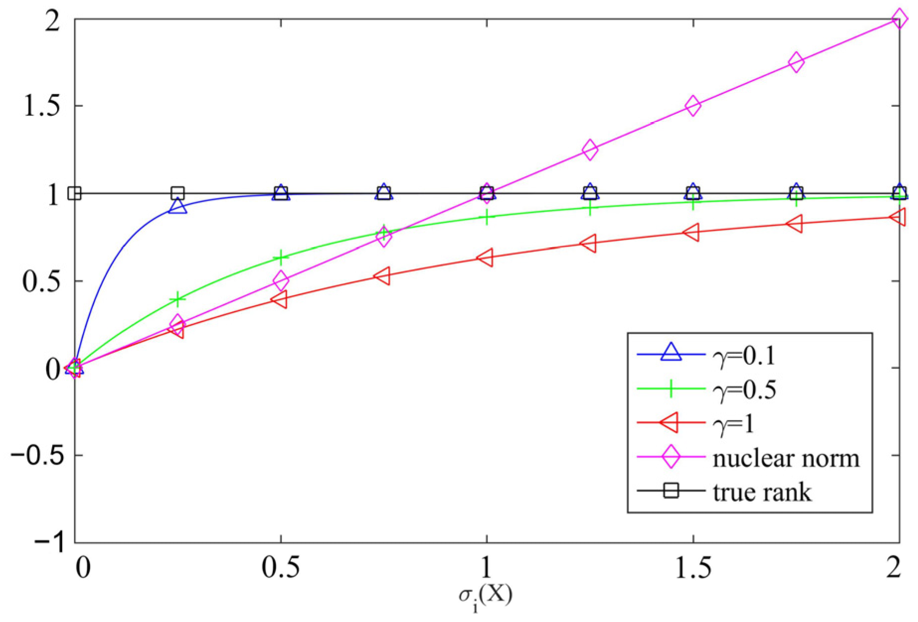
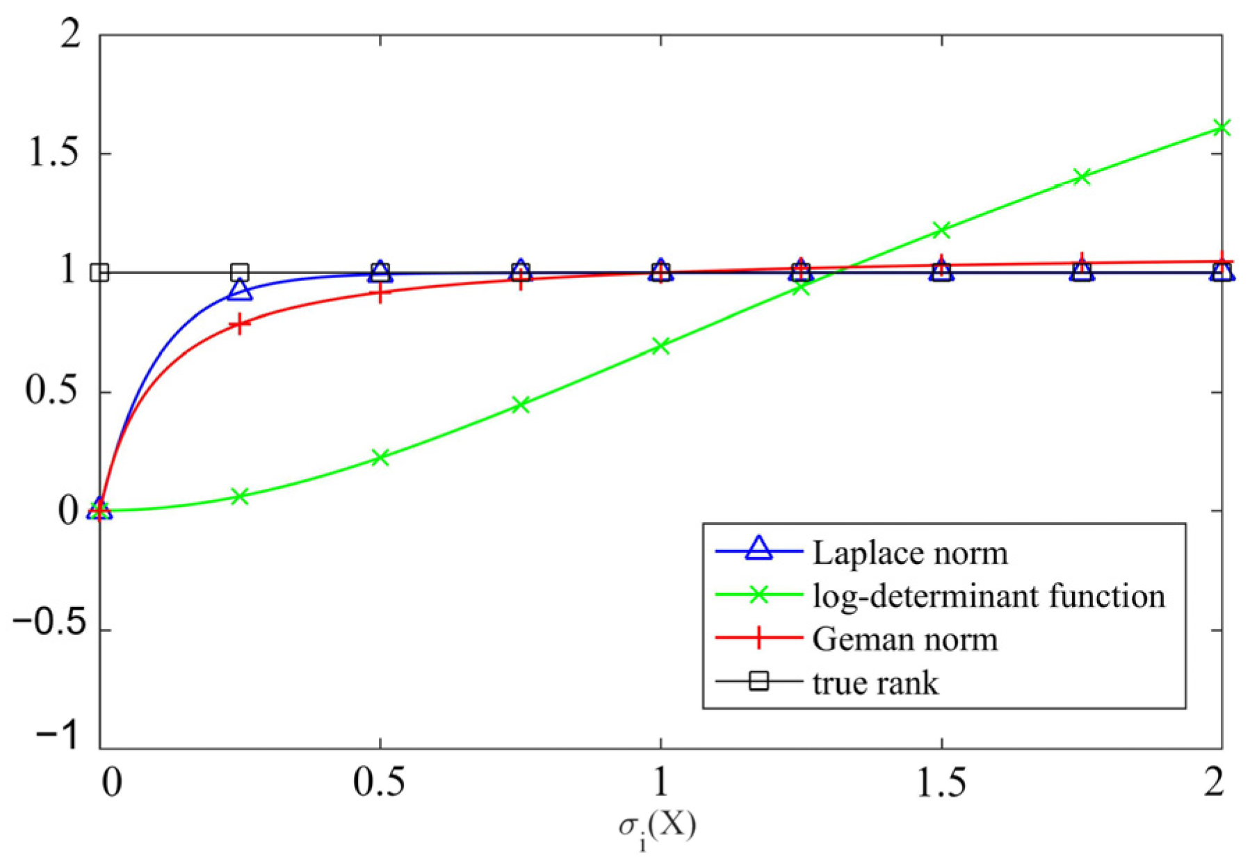
Based on the remarkable property in which the Laplace norm can effectively approximate the rank of a metric matrix, the non-convex metric learning method with nearest neighbor structure preservation and low-rank constraints is developed to optimize the metric matrix to improve the accuracy of the sample similarity metric in the process of trajectory feature encoding and clustering. The resultant non-convex issue can be efficiently addressed by leveraging the difference of convex functions algorithm (DCA) and alternating direction method of multipliers (ADMM) approaches.
(2)
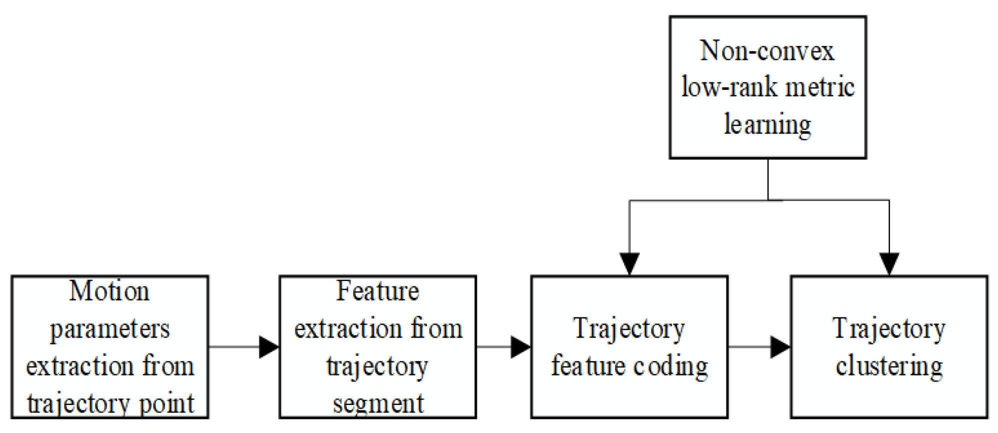
Raw trajectories can be divided into several homogeneity sub-trajectories based on the extracted kinematic parameters of trajectory points under the minimum description length principle, and its feature set is obtained by calculating the statistic characteristics of sub-trajectories.
(3)
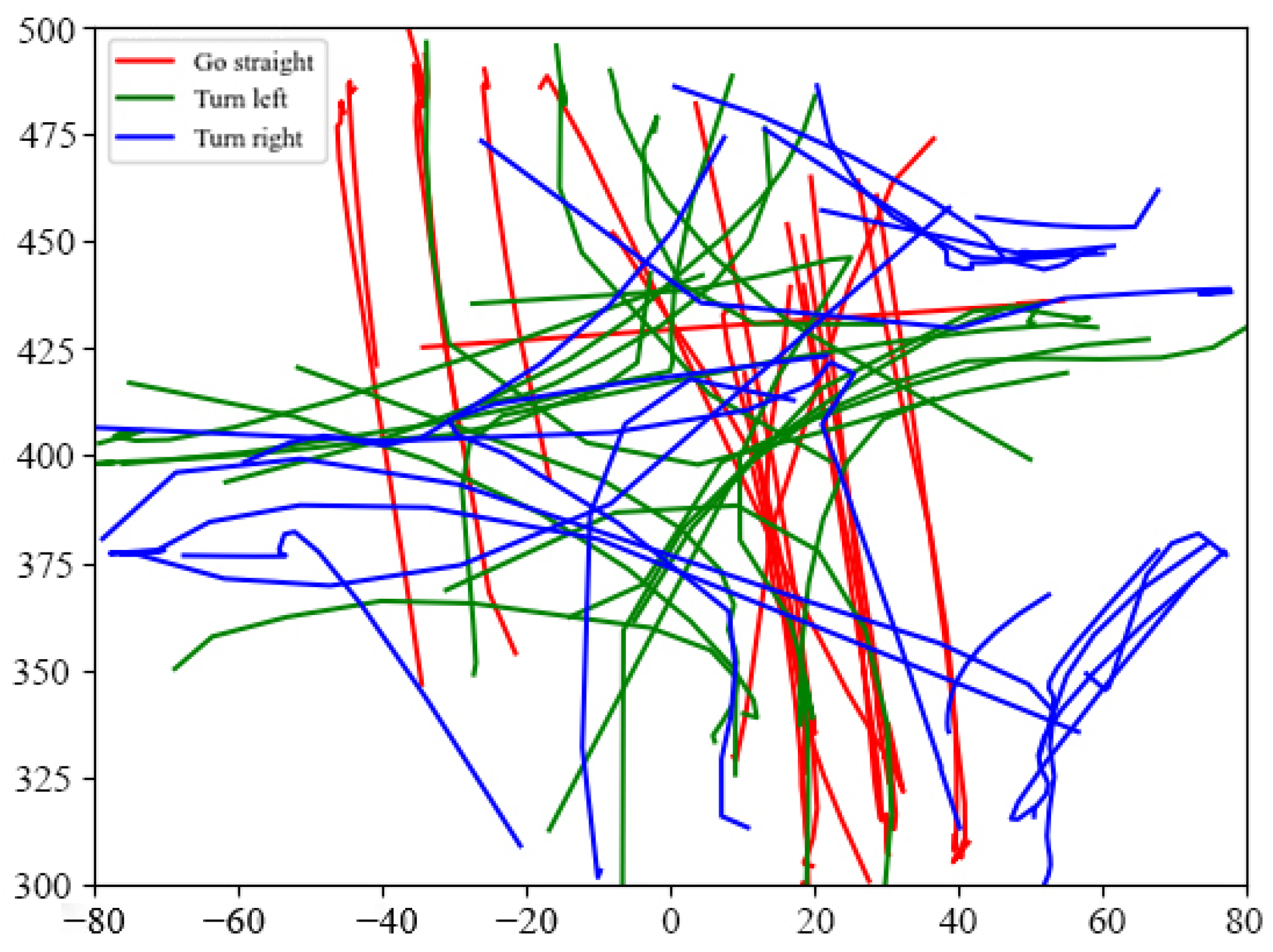
The segmented trajectory can be encoded as a fixed-length vector by leveraging the bag-of-words model, along with the developed metric learning method, to obtain its feature descriptor. Subsequently, all feature descriptors can be clustered using the K-means clustering algorithm in conjunction with the proposed metric learning approach, thereby facilitating effective trajectory clustering.
The remainder of this work is organized as follows: Section 2 presents the metric learning model incorporating manifold and low-rank constraints, along with an effective approach utilizing DCA and ADMM to address the resultant non-convex problem. In Section 3, we detail the extraction of trajectory point motion parameters, segment feature extraction, trajectory feature encoding, and clustering processes. The effectiveness of the proposed method is verified via numerical examples in Section 4. Finally, conclusions are drawn in Section 5.

2. Non-Convex Low-Rank Metric Learning

The overall framework of the proposed method is depicted in Figure 1. The proposed algorithm mainly comprises the following five modules: Firstly, based on the outstanding property in which Laplace norm can considerably approximate the rank of the metric matrix, the non-convex low-rank metric learning method is proposed to optimize the metric matrix, thereby enhancing the accuracy of the sample similarity metric during the trajectory feature encoding and clustering process; Furthermore, the motion parameters of trajectory points are extracted to obtain the features of each trajectory point; Moreover, the trajectory can be divided into several optimal homogeneous segments by applying the unsupervised segmentation algorithm, and the statistical features of each segment are extracted. In addition, the trajectory features can be encoded by employing the proposed metric learning method and bag-of-words model. Finally, trajectory clustering can be accomplished by using the proposed metric learning method and the K-means method.
The Laplace norm is initially introduced in this section. Subsequently, a metric learning model based on nearest neighbor structure preservation and low-rank constraints is elaborated. Finally, the DCA and ADMM approaches can be utilized to address the resulting optimization problem.

2.1. Laplace Norm

Assuming that the singular value decomposition (SVD) of the matrix X m × n can be expressed as X = U Σ V T , in which, U = u 1 , u 2 , , u r X and V = v 1 , v 2 , , v r X are the left and right singular matrices, respectively, = diag σ 1 , σ 2 , , σ r X is the diagonal matrix, σ 1 σ 2 σ r X 0 , r X is the rank of X , and σ i X is the i th singular value of X , then the Laplace norm of the matrix X can be defined as follows:
X γ = i = 1 r ϕ ( σ i ( X ) )
where ϕ ( σ i ( X ) ) = 1 e σ i ( X ) γ is the penalty function, and γ > 0 is the order of the Laplace norm.
It is known that the Laplace norm, X γ , is a pseudo-norm of the approximate L 0 norm [29], which has the following excellent properties: (1) rank approximation: lim γ 0 X γ = r a n k ( X ) ; (2) unitary invariance: for any unitary matrix U m × m , V n × n , X γ = U X V γ is satisfied; and (3) positivity: X γ 0 , when and only when X = 0 and X γ = 0 .
It is evident that the issue associated with the rank function, r a n k ( X ) , is a complicated non-convex problem that is difficult to solve directly, and therefore, the approximation method is usually used to achieve an effective solution [30]. The rank function approximation can be divided into the following two categories: convex and non-convex approximation. Among these, the commonly used convex approximation function is the kernel norm, and the kernel norm optimization can be considered a convex problem and, thereby, can be solved directly. Nevertheless, the kernel norm is a biased estimator, which might over-penalize large singular values, subsequently resulting in the inability of the kernel norm optimization to achieve the optimal solution. Meanwhile, the commonly exploited non-convex approximation functions include the Laplace norm, logarithmic determinant function, Geman norm, etc., which can be regarded as nearly unbiased estimations of the rank function, thus enhancing the accuracy of the solution to the rank optimization problem. To acquire a superior approximation of the rank function, Figure 2 and Figure 3 present the comparison curves of the approximation effects of the aforementioned functions. It can be observed from Figure 2 that the Laplacian norm can approximate the rank function more precisely with the increase in singular values compared to the kernel norm, and the approximation effect becomes better when γ = 0.1 . It is discernible from Figure 3 that the approximation effect of the Laplacian norm ( γ = 0.1 ) to the rank function is superior to that of other non-convex functions. Accordingly, the Laplace norm with γ = 0.1 can be selected to approximate the rank function.
To facilitate solving the non-convex problems associated with the Laplace norm, the definition of the subgradient of the Laplace norm can be given as follows:
X γ = U d i a g ( X ) V T : X i = d ( ϕ ( σ i ( X ) ) d ( σ i ( X ) ) , i = 1 , 2 , , r X
Based on Equation (1), the equation above can be rewritten as follows:
X γ = U d i a g ( X ) V T : X i = e σ i ( X ) γ γ , i = 1 , 2 , , r X

2.2. Metric Learning Manifold Constraints

It is well-known that metric learning plays a significant role in tasks such as classification, clustering, and information retrieval [2]. Existing metric learning methods can be classified into the following three categories: supervised, unsupervised, and semi-supervised metric learning. Among these, supervised metric learning utilizes all training sample label information to constrain the learning model, while unsupervised metric learning does not require any label information and aims at mining the potential low-dimensional manifold of the data to preserve the local topology to the greatest extent possible; thus, it can be expressed from the perspective of dimensionality reduction and manifold learning. Semi-supervised metric learning combines the advantages of both supervised and unsupervised metric learning by leveraging the geometric information of unlabeled samples and the label information of the limited labeled samples to learn distance metrics [31]. Considering that the training samples in clustering tasks usually do not contain label information, manifold learning can be exploited to measure sample similarity in this section. The manifold learning methods mainly include Laplacian eigenmaps (LE), locality preserving projections (LPP), and locally linear embedding (LLE), which can fully preserve the local structure information and maintain the nearest neighbor relationship of the data after dimensionality reduction [32]. Additionally, the following manifold assumption is proposed in [33]: if two samples have the nearest neighbor relationship in Euclidean space, the two also maintain this relationship in Mahalanobis space. Based on the mentioned above, metric learning with manifold constraints can be exploited here to improve the trajectory clustering performance.
Given a dataset, X sa = { X i } i = 1 n s a D , where n s a is the number of samples and D is the data dimension, the Mahalanobis distance between X i and X j can be expressed as follows:
d M 2 ( X i , X j ) = ( X i X j ) T M ( X i X j ) = X i X j M 2
where M D × D is the semi-positive definite metric matrix [17].
Accordingly, the unsupervised metric learning under the manifold constraint can be illustrated as follows:
i = 1 n 1 j = i + 1 n ( X i X j ) T M ( X i X j ) W i j
where W = W i j n × n is the weighted matrix, which characterizes the sample association relationship, i.e., the sample space manifold, and can be expressed as follows:
W i j = 1 , X i a n d X j h a v e c o n n e c t 0 , X i a n d X j d o n o t h a v e c o n n e c t
Based on the relevant property of the matrix trace, Equation (5) can be reformulated as follows:
i = 1 n 1 j = i + 1 n ( X i X j ) T M T ( X i X j ) W i j = i = 1 n 1 j = i + 1 n ( M ( X i X j ) ) T ( X i X j ) W i j = i = 1 n 1 j = i + 1 n t r ( M ( X i X j ) ( X i X j ) T ) W i j = i = 1 n 1 j = i + 1 n t r ( M C i j ) W i j
where C i j = ( X i X j ) ( X i X j ) T , t r ( · ) is the matrix trace operator.

2.3. Metric Matrix Low-Rank Constraint

It is known from [34,35] that the computational complexity of the metric learning algorithm is O ( D 2 ) at least, where D is the data dimension. This indicates that the high-dimensional metric matrix significantly increases the computational complexity. Additionally, full-rank metric learning is prone to causing model overfitting. Therefore, low-rank constrained metric matrix regularization is proposed in [18] to mitigate the computational complexity and prevent overfitting. However, a biased kernel norm rank approximation is utilized in [18], thereby limiting the improvement of metric performance. It is clear from the abovementioned that the Laplace norm can approximate the matrix rank more accurately and thus improve the accuracy of the regularized model. Consequently, the metric performance can be enhanced in this section based on the low-rank constraint of the Laplace norm.
With Equation (1), the Laplace norm of the matrix M can be depicted as follows:
M γ = i = 1 n ϕ ( σ i ( M ) )
As a consequence, the objective function associated with the Laplace norm of the metric matrix under the low-rank constraint can be constructed as follows:
min M M γ

2.4. Solving Metric Learning Issue with Low-Rank and Manifold Constraints

Based on (7) and (9), the metric learning issue under the low-rank and manifold constraints can be constructed as follows:
min M i = 1 n 1 j = i + 1 n t r ( M C i j ) W i j + λ M γ
where λ is the regularization parameter.
Obviously, model (10) is a rather complicated non-convex problem associated with M , which is difficult to solve directly by using traditional convex optimization methods. According to [36], DCA can linearize non-convex problems into convex ones and then solve them iteratively with global convergence, while ADMM can handle non-smooth issues with strong convergence. Therefore, the abovementioned complicated non-convex issue can be solved by using DCA and ADMM, and the proposed method consisting of DCA outer loop and ADMM inner loop can be illustrated as follows.
Outer loop: DCA decomposes the non-convex problem f ( M ) into the difference of two convex functions, i.e., g ( M ) h ( M ) . In addition, it is known from the definition of a subgradient that if h ( M ) exists a subgradient, it must satisfy the following conditions:
h ( M ) h ( M k ) + h ( M k ) , M M k
where k is the number of iterations, and h ( M k ) denotes the subgradient of h ( M ) at M k .
In one iteration, a linear approximation to h ( M ) in Equation (11) can be used to acquire a convex expression, and then the problem can be minimized and solved. Specifically, f ( M ) can be solved iteratively using the following model:
M k + 1 = arg min M g ( M ) ( h ( M k ) + h ( M k ) , M M k )
Thus, problem (10) can be solved iteratively based on the following function:
g ( M ) = i = 1 n 1 j = i + 1 n t r ( M C i j ) W i j h ( M ) = λ M γ
The optimization variables are iteratively updated as follows:
M k + 1 = arg min M i = 1 n 1 j = i + 1 n t r ( M C i j ) W i j + λ M k γ , M + C
where C = λ ( M k γ M k γ , M k ) .
Since M k is the last iterative solution, C is a constant; thus, the solution to issue (10) can be obtained by solving the following convex problem:
M k + 1 = arg min M i = 1 n 1 j = i + 1 n t r ( M C i j ) W i j + λ M k γ , M
It can be seen that problem (15) is non-smooth, and thus, no closed-form solution can be obtained directly [37], while it is known from the mentioned above that ADMM can solve the non-smooth problem effectively; thus, ADMM can be employed to solve this issue iteratively.
The termination condition of DCA can be expressed as follows [38]:
RelErr 1 = M k + 1 M k 2 max { M k 2 , 1 } ε outer
where · 2 is the Euclidean norm, max · is the taking maximum operator, and ε outer > 0 is the outer loop convergence threshold.
Inner loop: To facilitate solving the issue, the auxiliary variables, N , are introduced, and then issue (15) can be transformed into the following optimization problem with equation constraints:
arg min M i = 1 n 1 j = i + 1 n t r ( N C i j ) W i j + λ M k γ , M s . t .   M N = 0
The augmented Lagrangian function of the previous problem can be formulated as follows:
L ( M , N , Y , μ ) = i = 1 n 1 j = i + 1 n t r ( N C i j ) W i j + λ M k γ , M + Y , M N + μ 2 M N F 2
where Y is the Lagrange multiplier, and μ > 0 is the penalty parameter.
Issue (18) can be solved iteratively based on ADMM, which can be illustrated in detail as follows:
(1) Fixing M , the following optimization problem can be solved to update N :
N l + 1 = arg min N L ( M l , N , Y l , μ l )
that is,
N l + 1 = arg min N i = 1 n 1 j = i + 1 n t r ( N C i j ) W i j + λ M k γ , M l + Y l , M l N + μ l 2 M l N F 2
Discarding the terms independent of the optimization variables, (20) can be recast as follows:
N l + 1 = arg min N i = 1 n 1 j = i + 1 n t r ( N C i j ) W i j + μ l 2 M l N + Y l μ l F 2
Taking the derivative of the abovementioned object function and making it zero, one can obtain the following equation:
i = 1 n 1 j = i + 1 n C i j W i j Y l μ l ( M l N ) = 0
Then, the following equation can be obtained:
N l + 1 = M l + μ l 1 ( Y l i = 1 n 1 j = i + 1 n C i j W i j )
(2) Fixing N , the following optimization issue can be solved to update M :
M l + 1 = arg min M L ( M , N l + 1 , Y l , μ l )
that is,
M l + 1 = arg min M i = 1 n 1 j = i + 1 n t r ( N l + 1 C i j ) W i j + λ M k γ , M + Y l , M N l + 1 + μ l 2 M N l + 1 F 2
Discarding the term unrelated to the optimization variables, we have the following equation:
M l + 1 = arg min M λ M k γ , M + μ l 2 M N l + 1 + Y l μ l F 2
Similarly, one can obtain the following equation:
M l + 1 = N l + 1 μ l 1 Y l + λ M k γ
(3) Fixing M and N , Y can be updated using the following equation:
Y l + 1 = Y l + μ l ( M l + 1 N l + 1 )
Similar to DCA, the ADMM convergence condition can be set as follows:
RelErr 2 = M l + 1 M l 2 max { M l 2 , 1 } ε inner
where ε inner > 0 is the inner loop convergence threshold. Meanwhile, to speed up the iteration, the penalty parameter μ can be updated using the following equation:
μ l + 1 = min β μ l , μ max
where β ( 0 , 1 + 5 2 ) is the magnification, and μ max is the upper bound of μ l .
In summary, the specific steps of the proposed non-convex low-rank metric learning method are presented in Algorithm 1.
Algorithm 1. Non-convex low-rank metric learning method
Input: training samples X s a ,   ε inner ,   ε outer ,   μ max ,   β ,   λ
Initialization: M 0 = I   ( I D × D for unit matrix), k = 0 ,   l = 0 ,   Y 0 = 0 ,   μ 0
while RelErrl > ε outer do
        1 .   Calculate   M k γ with (3)
   while RelErr 2 > ε inner do
        2 .   Fixing   M k ,   update   N l with (23)
      3. Fixing N l ,   update   M l with (27)
      4. Fixing M l and N l ,   update   Y l with (28)
      5. Update penalty parameter μ l with (30)   
      6. l = l + 1
   end while
      7. M k + 1 = M l + 1
        8 .   k = k + 1
end while
Output:  M k + 1

3. Trajectory Clustering with the Bag-of-Words Model and Metric Learning

3.1. Trajectory Point Motion Parameters Extraction

Given a trajectory dataset, X t r = T r i i = 1 n t r , where n t r is the number of trajectories, the trajectory, T r i , is composed of a finite number of position vectors: T r i = p i , t 1 , , p i , t k , , p i , t n T , where p i , t k = ( x i , t k , y i , t k ) is the i th target position at the t k moment. Each trajectory point can calculate the corresponding motion parameters based on the time stamp and position information, i.e., velocity s i , t k , acceleration a i , t k , and steering angle r i , t k . Concretely, we obtain the following equations:
s i , t k = ( x i , t k x i , t k 1 ) 2 + ( y i , t k y i , t k 1 ) 2 t k t k 1
a i , t k = s i , t k s i , t k 1 t k t k 1
r i , t k = a r c t a n y i , t k y i , t k 1 x i , t k x i , t k 1
The steering angle of the first trajectory point of each trajectory can be set as r i , t 1 = 0 here.

3.2. Trajectory Segment Feature Extraction

As a fundamental step in motion data analysis, trajectory segmentation can divide the trajectory into several meaningful subsequences. Effective trajectory segmentation methods not only offer high-quality features to characterize the behavior of the moving target but also significantly reduce the computational complexity. Common trajectory segmentation methods can be categorized into the following three types: supervised, unsupervised, and semi-supervised trajectory segmentation. Supervised trajectory segmentation depends on predefined rules, labels, and thresholds. Nevertheless, the segmentation criteria cannot be specified in some cases and depend on the characteristics of the trajectory dataset. Unsupervised trajectory segmentation does not require target information and achieves segmentation only through the constructed cost function. Semi-supervised trajectory segmentation is a combination of supervised and unsupervised trajectory segmentation [39].
Since the trajectory data of the clustering task typically lacks label information, the trajectory can be segmented by employing the unsupervised trajectory segmentation algorithm GRASP-UTS proposed in [40]. Minimal distortion and maximal compression are exploited in GRASP-UTS to determine the optimality of the homogeneous segments. Specifically, achieving minimal distortion in trajectory segmentation requires that the trajectory segments display a high degree of homogeneity with respect to their characteristics, ensuring that points within each segment exhibit substantial similarity. Conversely, achieving maximal compression in trajectory segmentation entails minimizing the number of resultant trajectory segments, thereby optimizing the selection of landmarks. Consequently, the concepts of minimal distortion and maximal compression are orthogonal, that is, selecting all trajectory points as landmarks minimizes distortion but sacrifices compression efficiency. On the contrary, choosing a single landmark for the entire trajectory maximizes compression but introduces significant distortion.
From the description above, it is clear that the homogeneity and number of segments are dependent on the distortion and compression, while the clustering relies on the similarity between segments, which is influenced by the homogeneity; hence, the clustering results are inevitably affected by segmentation. In order to mitigate this effect as much as possible, the MDL principle is carefully designed in GRASP-UTS to achieve homogeneity in the segments.
According to the methods mentioned above, the main steps of the trajectory segmentation are briefly described below.
(1) Several sample trajectory reference points (representative feature points) can be randomly selected, and several continuous trajectory segments are generated in the vicinity of the reference points.
(2) A cost function is constructed under the MDL principle based on the characteristics of minimum distortion and maximum compression segmentation, and the resultant cost function is minimized to adjust the trajectory segment boundaries.
(3) The position and number of reference points can be iteratively updated, and steps (1)–(2) are executed until the best homogeneous trajectory segments can be obtained.
Several best homogeneous trajectory segments will be generated after segmentation, and each segment contains several trajectory points. Subsequently, the statistical features of each segment can be extracted based on the motion parameters of the acquired trajectory points, namely, minimum, maximum, mean, median, and standard deviation, to obtain the global features of the trajectory segments; that is, each segment can be represented by a 15-dimensional feature vector. Finally, each trajectory is characterized by the corresponding segment features. So far, all the trajectories in the X t r can acquire the corresponding feature set, T S = L i i = 1 n t r , after segmentation and statistic feature extraction, where L i is the i th trajectory feature. The number of segments for each trajectory, L i , may be different in T S , and the segments of each trajectory can comprise a segment feature set, L D = C i j , in which C i j is the i th segment statistical feature of the j th trajectory, i = 1 , , n t r . The value range of each trajectory, j , is different, which can be determined on the basis of the number of the corresponding segments. Additionally, T S and L D will be used to encode the trajectory feature.

3.3. Trajectory Feature Encoding

The bag-of-words model was originally proposed as a feature coding method for text retrieval, and nowadays, it is widely used in data mining, image processing, vision detection, and other fields [41]. The bag-of-words model can encode all trajectories with different lengths into fixed-length feature vectors, and the process is straightforward to implement. Therefore, trajectory features can be encoded by utilizing the improved bag-of-words model, which mainly consists of K-means-based dictionary generation and nearest neighbor search-based trajectory feature quantization. The dictionary generated by the former will be utilized in the search process of the latter for quantization. The encoding steps can be elaborated in detail as follows.
Dictionary generation:
(1) With the trajectory segment feature set, L D , the proposed low-rank metric learning method is used to obtain the metric matrix suitable for L D .
(2) Some L D samples can be randomly selected as the initial dictionary, i.e., the initial clustering prime.
(3) The Mahalanobis distance from other samples to the dictionary words can be calculated with the obtained metric matrix, and then they can be divided into clusters represented by the words under the principle of minimum distance, thereby obtaining several clusters.
(4) The mass center of each cluster can be recalculated as words.
(5) The sum of squared distances from each sample within the cluster to the mass center of the corresponding cluster, i.e., the sum of squared intra-cluster errors, is calculated. If it is less than the given threshold, the words of each cluster can be combined to construct the dictionary; otherwise, steps (2)–(4) need to be repeated.
Trajectory feature quantification:
(1) Initialize the trajectory feature vector as 0 , and the length of the vector is identical to the number of words in the obtained dictionary.
(2) Search all trajectory segments, L i , i = 1 , , n t r , which is essentially a nearest neighbor search process. Specifically, the dictionary words can be regarded as the reference point, the distances between trajectory segments and all words are calculated, and each segment is replaced with the corresponding word according to the nearest neighbor principle, and then the number of similar segments can be counted on the basis of the word order to acquire the feature histogram associated with L i , i.e., feature vector z i .
(3) All trajectory features within T S can be quantized to construct an encoding trajectory feature set, Z = z i i = 1 n t r , which will be exploited for the trajectory clustering.

3.4. Trajectory Clustering

The trajectories can be clustered after feature extraction and encoding, the main steps of which can be delineated as follows:
(1) The metric matrix suitable for Z can be obtained by using the developed non-convex low-rank metric learning algorithm with the trajectory encoding feature set Z .
(2) The trajectory similarity can be measured by using the obtained metric matrix, and the trajectory clusters G = g i i = 1 m can be achieved by exploiting the K-means algorithm, where g i is the centroid of the i th trajectory class, and m is the number of classes.
According to the description above, the proposed clustering algorithm with the bag-of-words model and metric learning is shown in Algorithm 2.
Algorithm 2. Bag-of-words model and metric learning-based clustering approach
Input: Trajectory dataset X t r
1. Extract trajectory point motion parameters based on Equations (31)–(33).
2. Segment trajectories by using GRASP-UTS, and extract trajectory segment features.
3. Encode trajectory features based on the bag-of-words model and the metric matrix obtained via the proposed low-rank metric learning method.
4. Cluster trajectories by employing K-means and the metric matrix acquired using the developed low-rank metric learning method.
Output: Trajectory class clusters G

3.5. Analysis of Computational Complexity

The computational complexity of the proposed method mainly involves the computation of (3), (23), (27), (28), and (30). Because (23) and (28) involve only basic matrix addition and subtraction, their computational cost is negligible. Therefore, the primary computational burden of the proposed algorithm lies in the calculation of the sub-gradients for (3) and (27). According to [42], the computational complexity of calculating the subgradient is O ( D r 2 ) , where D r is the rank of the data matrix. Therefore, the overall computational complexity of the proposed algorithm can be estimated as O ( D r 2 ) . As a comparison, all of the computational complexities of the comparative approaches, that is, Hausdorff, DTW, and LCSS, can be denoted as O ( D 2 ) , where D is the dimension of the data matrix [43]. Due to the rank of the matrix being less than or equal to its dimension, the computational complexity of the proposed method is reduced compared to that of the comparison algorithms.

4. Experimental and Simulation Analysis

4.1. Experimental Dataset and Environment

The Federal Highway Administration (FHWA) launched the next-generation simulation (NGSIM) program in 2005 to collect microscopic traffic data during different time periods of four road sections, including I-80, us101, lankershim, and Peachtree, which are captured by an overhead camera with a sampling interval of 0.1 s to obtain a vehicle trajectory dataset [44]. The trajectory data mainly includes information such as vehicle number, position, type, speed, and acceleration. The vehicle types include motorcycles, small cars, and trucks. Additionally, the speed limit of the lankershim section is 35 mph, the collection time of the lankershim dataset is from 8:30 a.m.–9:00 a.m., and the collection is situated at the intersection [45].
In this section, the Lankershim dataset is filtered according to the following requirements: (1) the ranges of the horizontal and vertical coordinates are X 80 , 80 ft and Y ( 300 , 500 ft ) , respectively, (2) small cars are taken as the study object, (3) several consecutive trajectory points contain different location information, (4) trajectory points with speed exceeding 35 mph are excluded, (5) data on each vehicle shall not be less than 10, and (6) trajectories outside the intersection area and abnormal trajectories are ruled out.
A total of 95 trajectories of straight, left-turn, and right-turn types are generated after filtering. Therefore, 20 trajectories of each type can be obtained, and the trajectories are smoothed with the Savitzky–Golay filter to filter out noise. The real trajectory dataset after processing is shown in Figure 4. The experimental environment is as follows: Intel Core i7-7700 3.60 Ghz processor and 8 GB of memory. The parameter values of the developed algorithm can be set as follows: γ = 0.1 , λ = 0 . 1 , β = 1.618 , μ 0 = 10 3 , μ max = 10 10 , and ε inner = ε outer = 10 3 .

4.2. Evaluation Metrics

Precision, recall, and accuracy are employed herein as evaluation metrics to verify the effectiveness of the proposed algorithm, and the relevant evaluation metrics are defined as follows [46].
It is known that the dataset, X t r , can be divided into k classes, i.e., T = T 1 , T j , T k , X t r can be clustered to produce r class clusters, i.e., C = C 1 , C i , , C r , and the relationship between r and k is indefinite. With this, one can obtain the following evaluation metrics:
The accuracy rate of the class cluster C i , Prec i , can be formulated as follows:
Prec i = 1 n i max j = 1 k n i j = n i j i n i
where n i = C i is the number of trajectories of C i , n i j = C i T j is the number of overlapping trajectories between C i and T j , and n i j i is the maximum number of trajectories of T j belonging to C i and T j .
The recall rate of the class cluster C i , recall i , can be depicted as follows:
recall i = n i j i T j i = n i j i m j i
where m j i = T j i is the number of trajectories of n i j i belonging to class T j .
The cluster accuracy rate of X t r can be expressed as follows:
Accuracy = j = 1 n i j i n t r

4.3. Simulation Results and Analysis

The effectiveness of the proposed algorithm is verified by comparing it with three types of trajectory clustering methods based on distance measurement, including the LCSS distance [10], SSPD distance [12], and Hausdorff distance [6], to measure trajectory similarity, and then the clustering can be achieved by using the K-Medoids (KM) approach with better noise robustness. The clustering results acquired by each algorithm are shown in Figure 5. It is obvious from Figure 5a–c that the upper left-turn trajectory (green) is clustered using LCSS + KM as the right-turn trajectory (blue), while the lower left-turn trajectory (blue) is clustered as the straight turn trajectory (red), the middle left-turn trajectory (green) is clustered using Hausdorff + KM as the straight turn trajectory (red), and the upper left-turn trajectory (blue) is clustered using SSPD + KM as the left-turn trajectory (green). It can be seen from Figure 5d that the proposed algorithm can more accurately gather the trajectories within different regions, such as the upper right and lower right-turn trajectories (blue trajectories). The findings mentioned above can be attributed to the following fact: the compared algorithms only extract some features, such as trajectory direction and shape, for clustering, and thus, the clustering performance is poor, while the developed approach exploits the optimized metric matrix and bag-of-words model to promote the feature coding performance and lifts the clustering effect based on the optimized metric matrix; therefore, the trajectory clustering performance of different regions can be improved significantly.
Table 1 presents the precision and recall rates (columns 2 to 4), as well as the accuracy rates (column 5), obtained by each algorithm. It is clear from Table 1 that the clustering accuracy of the compared algorithms is rather low due to the fact that LCSS + KM, Hausdorff + KM, and SSPD + KM only consider trajectory direction, position, and shape information, respectively. As for the developed method, it takes motion parameters, such as velocity, into account and optimizes the metric matrix, which can improve the clustering accuracy and thereby improve the ability to distinguish different types of trajectories. Moreover, compared to the comparison algorithms, the proposed approach has a higher recall rate for straight trajectories, which indicates that the clustering method with trajectory feature coding and shape information can achieve excellent clustering performance for linear trajectories. Furthermore, compared with straight trajectories, the clustering accuracy rate acquired via each algorithm in the cases of the left- and right-turn trajectories is poor because the left and right-turn trajectories are rather similar. According to the description above, it is known that the proposed algorithm has higher accuracy and recall rates compared to the comparison algorithms in the scenarios of straight and left-turn, as well as right-turn, trajectories.

5. Conclusions

A trajectory clustering approach with the bag-of-words model and metric learning was developed in this paper based on trajectory feature encoding and metric learning theory. The trajectory was segmented via the proposed method into several optimal homogeneous trajectory segments under the MDL principle, and then the statistic features of each segment were calculated to obtain the feature set of trajectory segments. Subsequently, a metric learning method was proposed under manifold and low-rank constraints to improve the similarity metric performance. Additionally, the segmented trajectory was encoded into a fixed-length vector by using the bag-of-words model and the proposed metric learning method to acquire its feature descriptor. Finally, the segmented trajectories were clustered with K-means and the proposed metric learning method to achieve effective trajectory clustering. The experimental results show that the proposed algorithm can cluster trajectories more preferably than the LCSS, SSPD, and Hausdorff distance metric-based methods in different regions, especially in the case of linear trajectory, and distinguish different types of trajectories more accurately. It is important to note that comparative experiments indicate a lower clustering accuracy rate for the proposed algorithm in scenarios involving left–right rotation trajectories, owing to the high degree of similarity between such trajectories. Furthermore, the presence of noise and data loss in trajectory datasets results in the clustering accuracy rate of the proposed algorithm reaching only 71%. Deep learning, due to its superior feature extraction capabilities, can effectively address these complex scenarios. Consequently, future research will integrate non-convex low-rank metric learning with deep learning to construct a non-convex low-rank deep metric learning model, thereby enhancing trajectory clustering accuracy in challenging environments.

Author Contributions

Investigation, formal analysis, methodology, software, writing, validation, and visualization—X.L.; Conceptualization, funding acquisition, resources, and supervision—H.W. All authors have read and agreed to the published version of the manuscript.

Funding

This work was supported in part by the National Natural Science Foundation of China under Grant 61301258, the Key projects of the Natural Science Foundation of Zhejiang Province under Grant LZ21F010002, the China Postdoctoral Science Foundation under Grant 2016M590218, and the Foundation of State Key Laboratory of Complex Electromagnetic Environment Effects on Electronics and Information System under Grant CEMEE2023K0301.

Data Availability Statement

The raw data supporting the conclusions of this article are available upon request from the corresponding author.

Conflicts of Interest

The authors declare no conflicts of interest.

References

  1. Xie, J.; Liu, X.; Wang, M. SFKNN-DPC: Standard deviation weighted distance based density peak clustering algorithm. Inf. Sci. 2024, 653, 119788. [Google Scholar] [CrossRef]
  2. Jiang, J.; Pan, D.; Ren, H.; Jiang, X.; Li, C.; Wang, J. Self-supervised trajectory representation learning with temporal regularities and travel semantics. In Proceedings of the 2023 IEEE 39th International Conference on Data Engineering (ICDE), Anaheim, CA, USA, 3–7 April 2023; pp. 843–855. [Google Scholar]
  3. Yang, Y.; Cai, J.; Yang, H.; Zhang, J.; Zhao, X. TAD: A trajectory clustering algorithm based on spatial-temporal density analysis. Expert Syst. Appl. 2020, 139, 112846. [Google Scholar] [CrossRef]
  4. Yang, J.; Liu, Y.; Ma, L.; Ji, C. Maritime traffic flow clustering analysis by density based trajectory clustering with noise. Ocean Eng. 2022, 249, 111001. [Google Scholar] [CrossRef]
  5. Yu, Q.; Luo, Y.; Chen, C.; Chen, S. Trajectory similarity clustering based on multi-feature distance measurement. Appl. Intell. 2019, 49, 2315–2338. [Google Scholar] [CrossRef]
  6. Sousa, R.S.D.; Boukerche, A.; Loureiro, A.A. Vehicle trajectory similarity: Models, methods, and applications. In ACM Computing Surveys (CSUR); Association for Computing Machinery: New York, NY, USA, 2020; pp. 1–32. [Google Scholar]
  7. Niu, X.; Chen, T.; Wu, C.Q.; Niu, J.; Li, Y. Label-based trajectory clustering in complex road networks. IEEE Trans. Intell. Transp. Syst. 2019, 21, 4098–4110. [Google Scholar] [CrossRef]
  8. Besse, P.C.; Guillouet, B.; Loubes, J.-M.; Royer, F. Review and perspective for distance-based clustering of vehicle trajectories. IEEE Trans. Intell. Transp. Syst. 2016, 17, 3306–3317. [Google Scholar] [CrossRef]
  9. Kumar, D.; Wu, H.; Rajasegarar, S.; Leckie, C.; Krishnaswamy, S.; Palaniswami, M. Fast and scalable big data trajectory clustering for understanding urban mobility. IEEE Trans. Intell. Transp. Syst. 2018, 19, 3709–3722. [Google Scholar] [CrossRef]
  10. Ma, D.; Fang, B.; Ma, W.; Wu, X.; Jin, S. Potential routes extraction for urban customized bus based on vehicle trajectory clustering. IEEE Trans. Intell. Transp. Syst. 2023, 24, 11878–11888. [Google Scholar] [CrossRef]
  11. Tao, Y.; Both, A.; Silveira, R.I.; Buchin, K.; Sijben, S.; Purves, R.S.; Laube, P.; Peng, D.; Toohey, K.; Duckham, M. A comparative analysis of trajectory similarity measures. GISci. Remote Sens. 2021, 58, 643–669. [Google Scholar] [CrossRef]
  12. Wang, S.; Bao, Z.; Culpepper, J.S.; Cong, G. A survey on trajectory data management, analytics, and learning. ACM Comput. Surv. 2021, 54, 39. [Google Scholar] [CrossRef]
  13. Yao, D.; Zhang, C.; Zhu, Z.; Huang, J.; Bi, J. Trajectory clustering via deep representation learning. In Proceedings of the 2017 International Joint Conference on Neural Networks (IJCNN), Anchorage, AK, USA, 14–19 May 2017; pp. 3880–3887. [Google Scholar]
  14. Zhong, C.; Cheng, S.; Kasoar, M.; Arcucci, R. Reduced-order digital twin and latent data assimilation for global wildfire prediction. Nat. Hazards Earth Syst. Sci. 2023, 23, 1755–1768. [Google Scholar] [CrossRef]
  15. Taghizadeh, S.; Elekes, A.; Schäler, M.; Böhm, K. How meaningful are similarities in deep trajectory representations? Inf. Syst. 2021, 98, 101452. [Google Scholar] [CrossRef]
  16. Liang, M.; Liu, R.W.; Li, S.; Xiao, Z.; Liu, X.; Lu, F. An unsupervised learning method with convolutional auto-encoder for vessel trajectory similarity computation. Ocean Eng. 2021, 225, 108803. [Google Scholar] [CrossRef]
  17. Michelioudakis, E.; Artikis, A.; Paliouras, G. Online semi-supervised learning of composite event rules by combining structure and mass-based predicate similarity. Mach. Learn. 2024, 113, 1445–1481. [Google Scholar] [CrossRef]
  18. Sun, P.; Yang, L. Low-rank supervised and semi-supervised multi-metric learning for classification. Knowl. Based Syst. 2022, 236, 107787. [Google Scholar] [CrossRef]
  19. Macqueen, J. Some methods for classification and analysis of multivariate observations. In Proceedings of the Fifth Berkeley Symposium on Mathematical Statistics and Probability; University of California Press: Berkeley, CA, USA, 1967; Volume 233, pp. 281–297. [Google Scholar]
  20. Zhang, T.; Ramakrishnan, R.; Livny, M. BIRCH: An Efficient Data Clustering Databases Method for Very Large Databases. In Proceedings of the ACM SIGMOD International Conference on Management of Data, Montreal, QC, Canada, 4–6 June 1996; pp. 103–114. [Google Scholar]
  21. Wang, W.; Yang, J.; Muntz, R. STING: A Statistical Information Grid Approach to Spatial Data Mining. In Proceedings of the 23rd International Conference on Very Large Data Bases, Athens, Greece, 25–29 August 1997; pp. 186–195. [Google Scholar]
  22. Sheikholeslami, G.; Chatterjee, S.; Zhang, A. WaveCluster: A wavelet-based clustering approach for spatial data in very large databases. VLDB J. 2000, 8, 289–304. [Google Scholar] [CrossRef]
  23. Fisher, D. Knowledge acquisition via incremental clustering. Mach. Learn. 1987, 2, 139–182. [Google Scholar] [CrossRef]
  24. Ester, M.; Kriegel, H.P.; Sander, J.; Xu, X. A density-based algorithm for discovering clusters in large spatial databases with noise. In Proceedings of the Second International Conference on Knowledge Discovery and Data Mining, Portland, OR, USA, 2–4 August 1996; pp. 226–231. [Google Scholar]
  25. Ankerst, M.; Breunig, M.M.; Kriegel, H.; Sander, J. OPTICS: Ordering Points To Identify the Clustering Structure. In Proceedings of the 1999 ACM SIGMOD International Conference on Management of Data, Philadelphia, PA, USA, 1–3 June 1999; Volume 28, pp. 49–60. [Google Scholar]
  26. Ma, S.; Wang, T.; Tang, S.; Yang, D.; Gao, J. A New Fast Clustering Algorithm Based on Reference and Density. In Advances in Web-Age Information Management; Springer: Berlin/Heidelberg, Germany, 2002; pp. 214–225. [Google Scholar]
  27. Agrawal, K.P.; Garg, S.; Sharma, S.; Patel, P. Development and validation of OPTICS based spatio-temporal clustering technique. Inf. Sci. 2016, 369, 388–401. [Google Scholar] [CrossRef]
  28. Hüsch, M.; Schyska, B.U.; Bremen, L.V. CorClustST-Correlation-based clustering of big spatio-temporal datasets. Future Gener. Comput. Syst. 2020, 110, 610–619. [Google Scholar] [CrossRef]
  29. Huang, L.; Xu, Z.; Zhang, Z.; He, Y.; Zan, M. A fast iterative shrinkage/thresholding algorithm via laplace norm for sound source identification. IEEE Access 2020, 8, 115335–115344. [Google Scholar] [CrossRef]
  30. Greenacre, M.; Groenen, P.; Hastie, T.; d’Enza, A.I.; Markos, A.; Tuzhilina, E. Principal component analysis. Nat. Rev. Methods Primers 2022, 2, 1–100. [Google Scholar] [CrossRef]
  31. Yuan, C.; Yang, L. An efficient multi-metric learning method by partitioning the metric space. Neurocomputing 2023, 529, 56–79. [Google Scholar] [CrossRef]
  32. Lei, C.; Zhu, X. Unsupervised feature selection via local structure learning and sparse learning. Multimedia Tools Appl. 2018, 77, 29605–29622. [Google Scholar] [CrossRef]
  33. Islam, A.; Radke, R. Weakly supervised temporal action localization using deep metric learning. In Proceedings of the IEEE/CVF Winter Conference on Applications of Computer Vision, Waikoloa, HI, USA, 3–8 January 2020; pp. 547–556. [Google Scholar]
  34. Sun, G.; Cong, Y.; Wang, Q.; Xu, X. Online low-rank metric learning via parallel coordinate descent method. In Proceedings of the 2018 24th International Conference on Pattern Recognition (ICPR), Beijing, China, 20–24 August 2018; pp. 207–212. [Google Scholar]
  35. Chen, S.; Shen, Y.; Yan, Y.; Wang, D.; Zhu, S. Cholesky Decomposition-Based Metric Learning for Video-Based Human Action Recognition. IEEE Access 2020, 8, 36313–36321. [Google Scholar] [CrossRef]
  36. Ma, X.; Li, G.; Wang, Y.; Li, H.; Yang, W. Seismic Deconvolution Based on a Non-Convex L1-L2 Norm Constraint. In Proceedings of the 81st EAGE Conference and Exhibition, London, UK, 3–6 June 2019; pp. 1–5. [Google Scholar]
  37. Tono, K.; Takeda, A.; Gotoh, J. Efficient DC algorithm for constrained sparse optimization. arXiv 2017, arXiv:1701.08498. [Google Scholar]
  38. Wang, J.; Zhang, F.; Huang, J.; Wang, W.; Yuan, C. A nonconvex penalty function with integral convolution approximation for compressed sensing. Signal Process. 2019, 158, 116–128. [Google Scholar] [CrossRef]
  39. Junior, A.S.; Times, V.C.; Renso, C.; Matwin, S.; Cabral, L.A. A semi-supervised approach for the semantic segmentation of trajectories. In Proceedings of the 2018 19th IEEE International Conference on Mobile Data Management (MDM), Aalborg, Denmark, 25–28 June 2018; pp. 145–154. [Google Scholar]
  40. Etemad, M.; Júnior, A.S.; Hoseyni, A.; Rose, J.; Matwin, S. A Trajectory Segmentation Algorithm Based on Interpolation-based Change Detection Strategies. In Proceedings of the EDBT/ICDT Workshops, Lisbon, Portugal, 26 March 2019; pp. 51–58. [Google Scholar]
  41. Nivash, S.; Ganesh, E.N.; Harisudha, K.; Sreeram, S. Extensive analysis of global presidents’ speeches using natural language. In Sentimental Analysis and Deep Learning: Proceedings of ICSADL; Springer: Singapore, 2022; pp. 829–850. [Google Scholar]
  42. Mateos-Nunez, D.; Cortes, J. Distributed saddle-point subgradient algorithms with Laplacian averaging. IEEE Trans. Autom. Control 2016, 62, 2720–2735. [Google Scholar] [CrossRef]
  43. Liang, M.; Liu, R.W.; Gao, R.; Xiao, Z.; Zhang, X.; Wang, H. A survey of distance-based vessel trajectory clustering: Data pre-processing, methodologies, applications, and experimental evaluation. arXiv 2024, arXiv:2407.11084. [Google Scholar]
  44. Feng, X.; Cen, Z.; Hu, J.; Zhang, Y. Vehicle trajectory prediction using intention-based conditional variational autoencoder. In Proceedings of the 2019 IEEE Intelligent Transportation Systems Conference (ITSC), Auckland, New Zealand, 27–30 October 2019; pp. 3514–3519. [Google Scholar]
  45. Zhang, H.; Fu, R. A Hybrid Approach for Turning Intention Prediction Based on Time Series Forecasting and Deep Learning. Sensors 2020, 20, 4887. [Google Scholar] [CrossRef]
  46. Ghazal, T.M.; Hussain, M.Z.; Said, R.A.; Nadeem, A.; Hasan, M.K.; Ahmad, M.; Khan, M.A.; Naseem, M.T. Performances of k-means clustering algorithm with different distance metrics. Intell. Autom. Soft Comput. 2021, 29, 735–742. [Google Scholar] [CrossRef]
Figure 1. Trajectory clustering method based on bag-of-words model and metric learning.
Mathematics 13 00387 g001
Figure 2. Comparison of different-order Laplace and kernel parametric rank function approximation.
Mathematics 13 00387 g002
Figure 3. Comparison of common non-convex rank approximation functions.
Mathematics 13 00387 g003
Figure 4. Visualization of real trajectory dataset.
Mathematics 13 00387 g004
Figure 5. Visualization of clustering results.
Mathematics 13 00387 g005aMathematics 13 00387 g005b
Table 1. Comparison of clustering performance for real data sets.
Clustering MethodStraightLeft TurnRight TurnAccuracy
LCSS + KM0.70/0.480.40/0.530.45/0.5651.67%
Hausdorff + KM0.65/0.650.45/0.390.60/0.7156.67%
SSPD + KM0.85/0.680.65/0.590.45/0.6965.00%
The proposed algorithm0.90/0.950.57/0.600.55/0.5571.67%
Disclaimer/Publisher’s Note: The statements, opinions and data contained in all publications are solely those of the individual author(s) and contributor(s) and not of MDPI and/or the editor(s). MDPI and/or the editor(s) disclaim responsibility for any injury to people or property resulting from any ideas, methods, instructions or products referred to in the content.

