Article

Selkov’s Dynamic System of Fractional Variable Order with Non-Constant Coefficients

Laboratory of Physical Process Modeling, Institute of Cosmophysical Research and Radio Wave Propagation FEB RAS, 684034 Paratunka, Russia
Mathematics 2025, 13(3), 372; https://doi.org/10.3390/math13030372
Submission received: 30 December 2024 / Revised: 18 January 2025 / Accepted: 23 January 2025 / Published: 23 January 2025
(This article belongs to the Section C2: Dynamical Systems)

Abstract

:
This article uses an approach based on the triad model–algorithm–program. The model is a nonlinear dynamic Selkov system with non-constant coefficients and fractional derivatives of the Gerasimov–Caputo type. The Adams–Bashforth–Multon numerical method from the predictor–corrector family of methods is selected as an algorithm for studying this system. The ABMSelkovFracSim 1.0 software package acts as a program, in which a numerical algorithm with the ability to visualize the research results is implemented to build oscillograms and phase trajectories. Examples of the ABMSelkovFracSim 1.0 software package operation for various values of the model parameters are given. It is shown that with an increase in the values of the parameter responsible for the characteristic time scale, regular and chaotic modes are observed. Further in this work, bifurcation diagrams are constructed, which confirm this. Aperiodic modes are also detected and a singularity is revealed.

1. Introduction

Dynamic systems play an important role in various fields of knowledge, and it often happens that the same dynamic system of different nature can describe similar processes. The Selkov dynamic system is no exception. It is often encountered in biology when studying glycolytic reactions that have self-oscillatory modes [1].
The article by [2] proposed the use of the Selkov dynamic system to describe self-oscillatory modes of microseisms—small-amplitude oscillations of the earth’s surface, the source of which are natural and man-made processes.
In the work [3,4], a generalization of a dynamic system to the case of heredity is carried out. A property of a dynamic system is retaining the memory of its evolution, i.e., the current state of the system depends on its previous states. It is known that viscoelastic and plastic media can have heredity, and they are considered within the framework of hereditary mechanics [5]; heredity naturally arises in biology during the spread of viruses [6], and in economics to describe cycles and crises [7]. From a mathematical point of view, heredity in the general case can be described using Volterra-type integro-differential equations [8], and under certain conditions using derivatives of fractional constants or variables of order, which are studied within the framework of the theory of fractional calculus [9,10]. Therefore, we will further call Selkov’s dynamic system with fractional derivatives a fractional dynamic Selkov system.
A quantitative and qualitative analysis of the Selkov dynamic system with constant coefficients, taking into account heredity, which was described using derivatives of fractional constant orders in the Gerasimov–Caputo sense, was carried out. The following aspects of this dynamic system were investigated: equilibrium points, spectra of maximum Lyapunov exponents, and the development of a numerical algorithm based on the Adams–Bashforth–Multon method. The main results of the study were presented in the article [4]. Further, in the articles [11,12], a generalization of the Selkov system with constant coefficients was carried out for the case of derivatives of fractional variables of the Gerasimov–Caputo type. Numerical algorithms for finding a solution to the system were developed, and the Test 0-1 algorithms were applied to study regular and chaotic regimes.
In this paper, within the framework of the triad model–algorithm–program, a further generalization of the fractional dynamic Selkov system is proposed, associated with the dependence of its coefficients on time and on a certain parameter—the characteristic time scale. To obtain a solution to the generalized dynamic Selkov system, the Adams–Bashforth–Multon numerical algorithm is used, which was adapted for it. Then, based on the previously obtained results, as well as new results, the ABMSelkovFracSim 1.0 software package is developed in the Python programming language [13] in the PyCharm environment [14]. Then, using the software package, calculations of oscillograms and phase trajectories are carried out, characterizing various dynamic modes on bifurcation diagrams.
The research plan in this article has the following structure: the introduction reveals the problems of the article, Section 2 provides a description of the fractional dynamic Selkov system with non-constant coefficients, Section 3 provides a numerical algorithm for solving the proposed system based on the Adams–Bashforth–Multon method, Section 4 describes the software package in which the numerical algorithm is implemented, Section 5 provides examples of the software package operation, Section 6 studies bifurcation diagrams for various parameters of the system under study using the software package, and Section 7 provides conclusions based on the research results.

2. Statement of the Problem

Consider the following dynamic system:
0 t α 1 t x t = v 1 t x t + w 1 t y t + h 1 t x 2 t y t , x 0 = x 0 , 0 t α 2 t y t = v 2 t w 2 t y t h 2 t x 2 t y t , y 0 = y 0 .
where x t , y t C 1 0 , T —solution functions; v 1 t = θ 1 α 1 t , v 2 t = v 0 θ 1 α 2 t , w 1 t = w 0 θ 1 α 1 t , w 2 t = w 0 θ 1 α 2 t , h 1 t = h 0 θ 1 α 1 t , h 2 t = h 0 θ 1 α 2 t —functions from class C 0 , T ; θ —parameter with time dimension; v 0 , w 0 , h 0 —given constants; t 0 , T —current process time; T > 0 —simulation time; x 0 , y 0 —positive constants responsible for the initial conditions. Fractional derivative operators have the following form:
0 t α 1 t x ( t ) = 1 Γ ( 1 α 1 t ) 0 t x ˙ ( τ ) d τ ( t τ ) α 1 t , 0 t α 2 t y ( t ) = 1 Γ ( 1 α 2 t ) 0 t y ˙ ( τ ) d τ ( t τ ) α 2 t ,
which is understood in the sense of Gerasimov–Caputo [15,16], the orders of which are 0 < α 1 t , α 2 t < 1 , functions from the class C 0 , T .
Definition 1. 
We will call the system (1) a fractional dynamic Selkov system with variable memory or simply a fractional dynamic Selkov system.
Definition 2. 
The system (1) with the parameter value α 1 t = α 2 t = 1 will be called the classical dynamic Selkov system.
Remark 1. 
The parameter θ has the dimension of time; it determines a certain characteristic time scale in the process under consideration [17], and also coordinates the dimensions between the left and right parts of the equations in the system (1). Note that if θ = 1 in the system (1), then we arrive at the results of [11,12]. If the orders of the fractional derivatives α 1 t and α 2 t do not depend on time t and θ = 1 , then we arrive at the fractional dynamic Selkov system considered in the author’s articles [3,4]. In the case where α 1 = α 2 = 1 , we obtain the classical dynamic Selkov system [1].
Remark 2. 
Note that more detailed information on fractional derivatives of variable order can be found in the review articles [18,19].

3. Adams–Bashforth–Multon Method

To study the fractional dynamical Selkov system (1), we use the Adams–Bashforth–Moulton numerical method from the family of predictor–corrector methods. The Adams–Bashforth–Moulton method has been studied and discussed in detail in [20,21,22]. We adapt this method to solve the fractional dynamical Selkov system (1). To do this on a uniform grid N with step τ = T / N , we introduce the functions x k + 1 p , y k + 1 p , k = 0 , , N 1 , which will be determined by the Adams–Bashforth formula (predictor):
x k + 1 p = x 0 + τ α 1 , k Γ α 1 , k + 1 j = 0 k θ j , k + 1 1 v 1 , j x j + w 1 , j y j + h 1 , j x j 2 y j , y k + 1 p = y 0 + τ α 2 , k Γ α 2 , k + 1 j = 0 k θ j , k + 1 2 v 2 , j w 2 , j y j h 2 , j x j 2 y j , θ j , k + 1 i = k j + 1 α i , k k j α i , k , i = 1 , 2 .
For the corrector (Adams–Moulton formula), we obtain
x k + 1 = x 0 + K 1 , k v 1 , k + 1 x k + 1 p + w 1 , k + 1 y k + 1 p + h 1 , k + 1 x k + 1 p 2 y k + 1 p + + K 1 . k j = 0 k ρ j , k + 1 1 v 1 , j x j + w 1 , j y j + h 1 , j x j 2 y j , y k + 1 = y 0 + K 2 , k v 2 , k + 1 w 2 , k + 1 y k + 1 p h 2 , k + 1 x k + 1 p 2 y k + 1 p + + K 2 , k j = 0 k ρ j , k + 1 2 v 2 , j w 2 , j y j h 2 , j x j 2 y j .
where K 1 , k = τ α 1 , k Γ α 1 , k + 2 , K 2 , k = τ α 2 , k Γ α 2 , k + 2 , and weight coefficients in (3) are determined by the following formula:
ρ j , k + 1 i = k α i , k + 1 k α i , k k + 1 α i , k , j = 0 , k j + 2 α i , k + 1 + k j α i , k + 1 2 k j + 1 α i , k + 1 , 1 j k , 1 , j = k + 1 , i = 1 , 2 .
Remark 3. 
A study of the properties of the Adams–Bashforth–Multon method was carried out in a previous article [11].

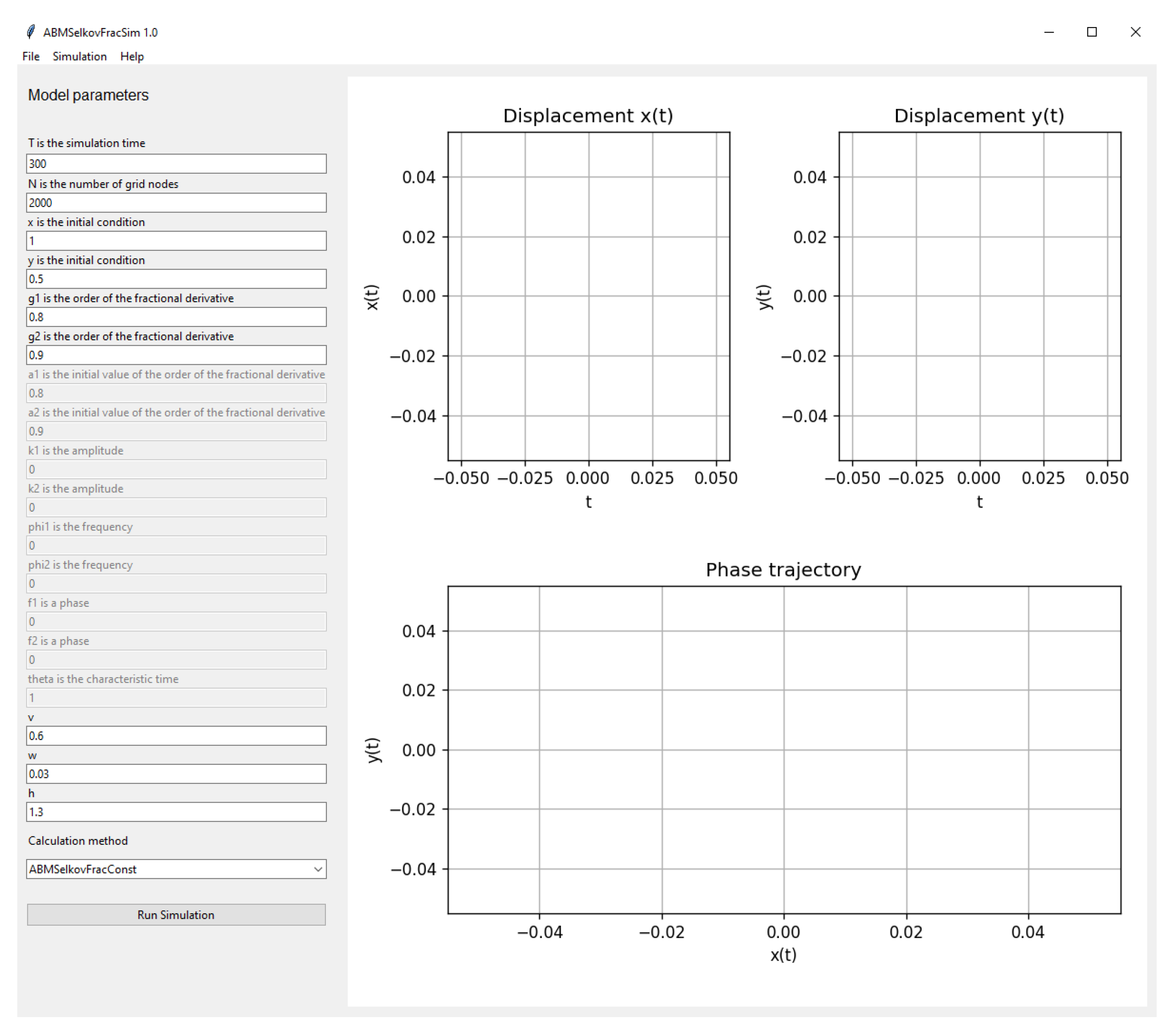
4. Software Package ABMSelkovFracSim

The Adams–Bashforth–Multon numerical algorithm (2), (3) is implemented in the Python programming language in the PyCharm 2024.1 environment in the form of the ABMSelkovFracSim software package. The ABMSelkovFracSim application has a clear user interface (Figure 1).
The user can enter the values of the parameters of the fractional dynamic Selkov system (1) in the left part of the interface, and the right part has the ability to visualize the simulation results: oscillograms and phase trajectories are displayed.
The ABMSelkovFracSim application has the ability to perform calculations using the model (1) (ABMSelkovFracConst method), as well as the model proposed in the article [4] (ABMSelkovFracCos method). The ABMSelkovFracConst method implements the case where the orders of the fractional derivatives α 1 and α 2 are constants.
In the ABMSelkovFracCos method, the orders of fractional derivatives are functions of the form
α 1 t = α 1 k 1 cos ( ϕ 2 + f 1 ) , α 2 t = α 2 k 2 cos ( ϕ 2 + f 2 ) ,
where α 1 , α 2 are given constants, k 1 , k 2 are amplitudes, ϕ 1 , ϕ 2 are frequencies, and f 1 , f 2 are phases.

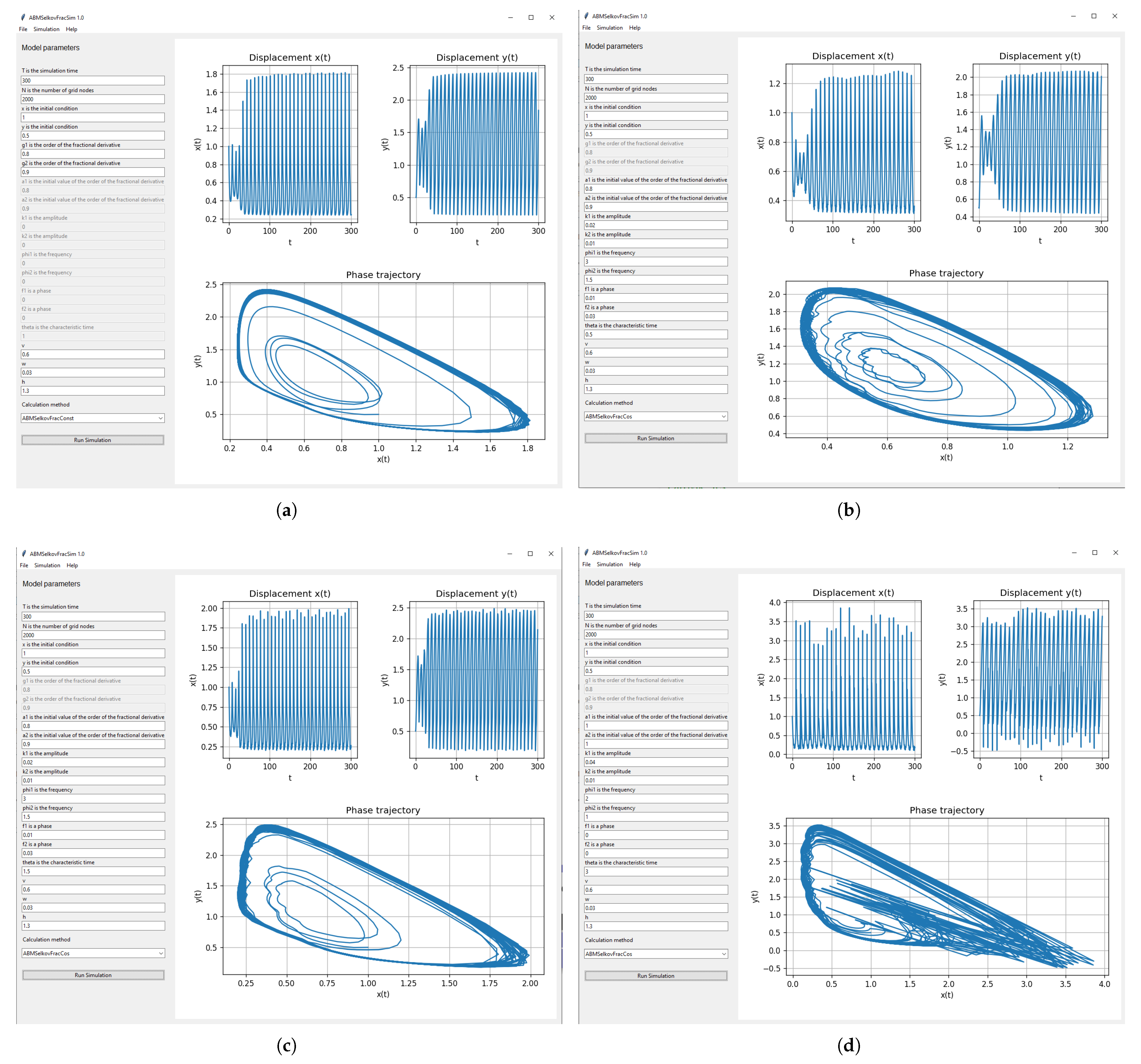
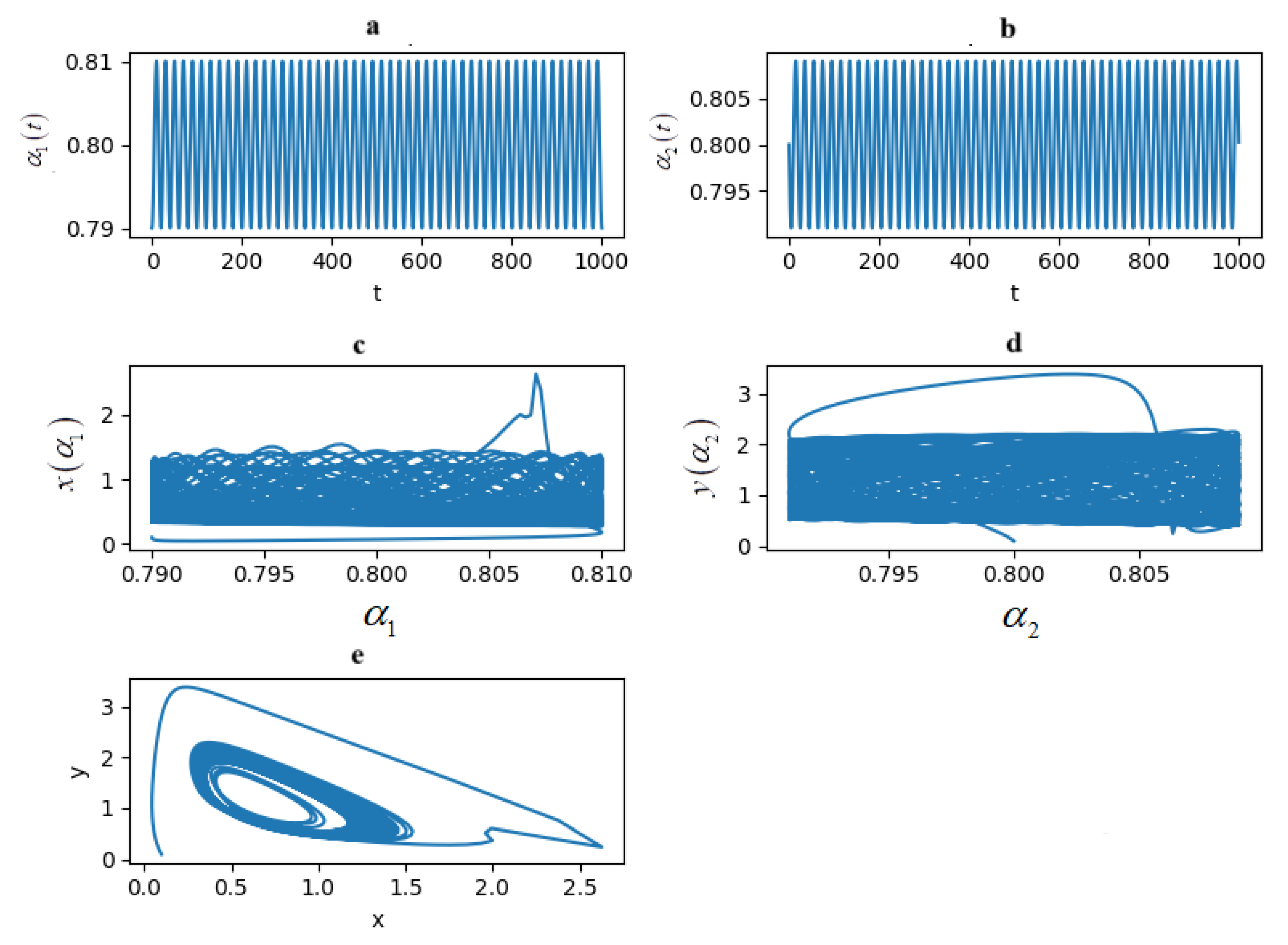
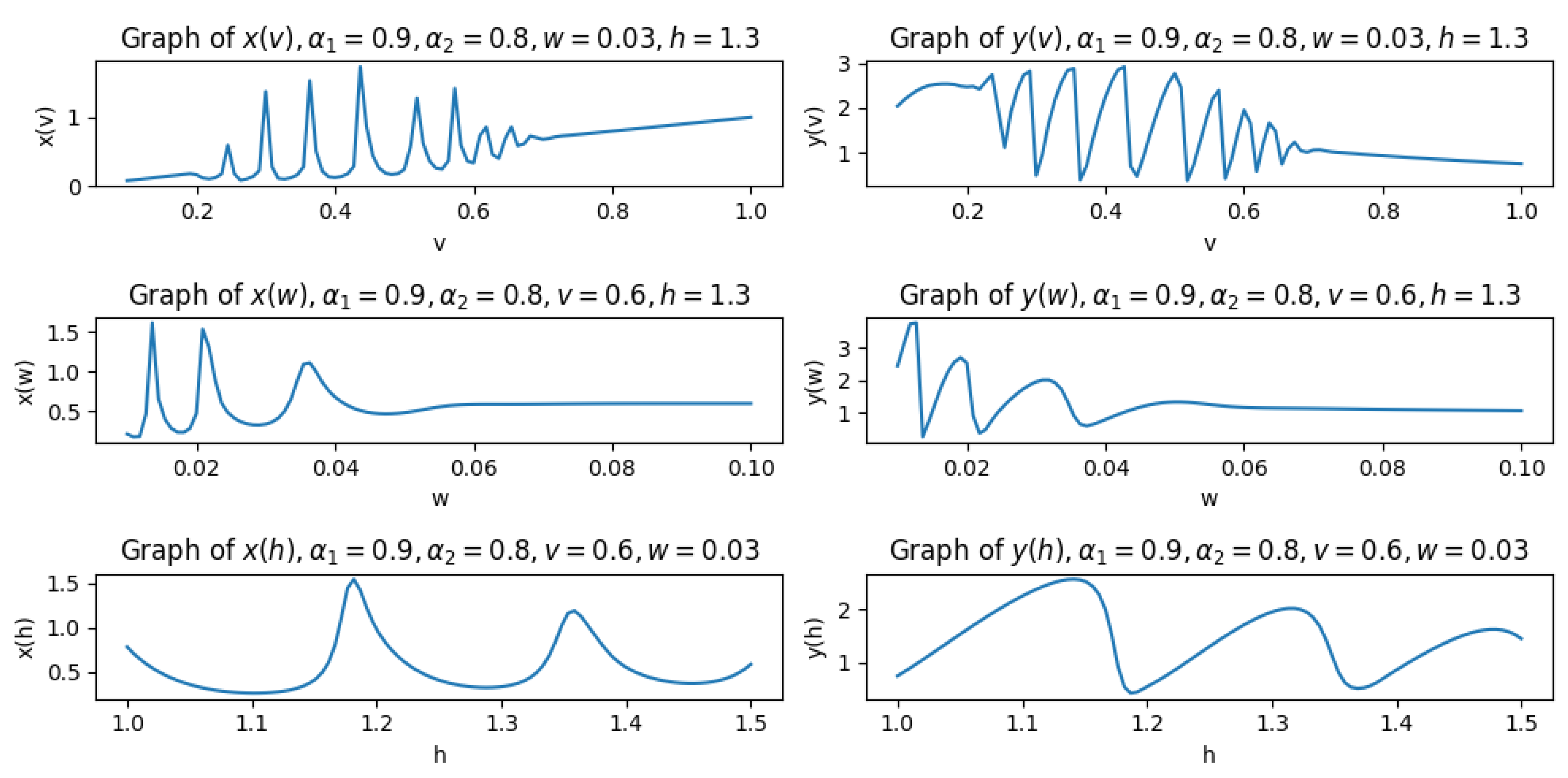
5. Simulation Results

Using the ABMSelkovFracSim software package, we will calculate oscillograms and phase trajectories for different values of θ . We will select the following parameters for calculation within the framework of the fractional dynamic Selkov system: v 0 = 0.6 , w 0 = 0.03 ,   h 0 = 1.3 ,   x 0 = 1 , y 0 = 0.5 ,   t 0 , 300 , N = 2000 (Figure 2).
Figure 2a shows the case obtained by the ABMSelkovFracConst method, when the orders of the fractional derivatives α 1 t and α 2 t are constants and the value of the parameter θ = 1 . This case was considered in the article [4]. The remaining graphs (Figure 2b–d) correspond to the case when α 1 t and α 2 t are functions and are constructed by the ABMSelkovFracCos method for different values of the parameter θ .
We see that with increasing values of θ , a transition from regular to chaotic modes occurs. Therefore, we need to analyze dynamic modes. We will analyze them using the construction of bifurcation diagrams.

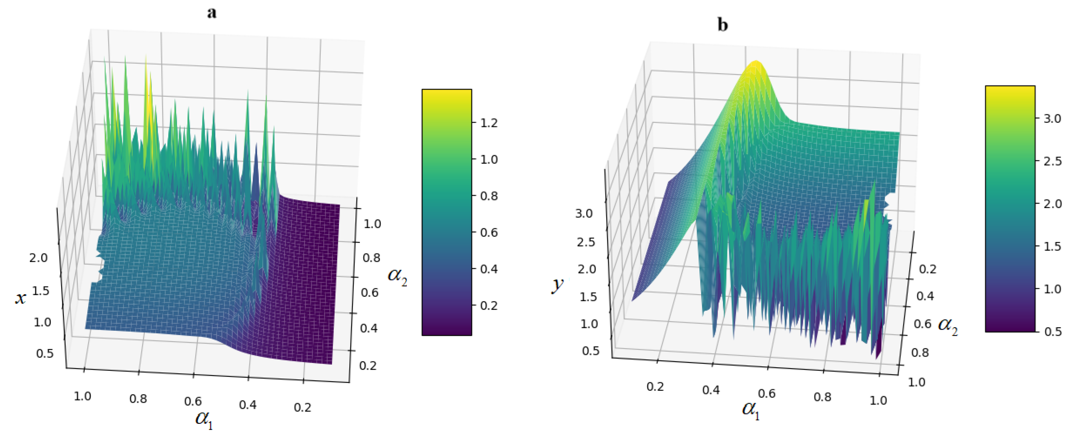
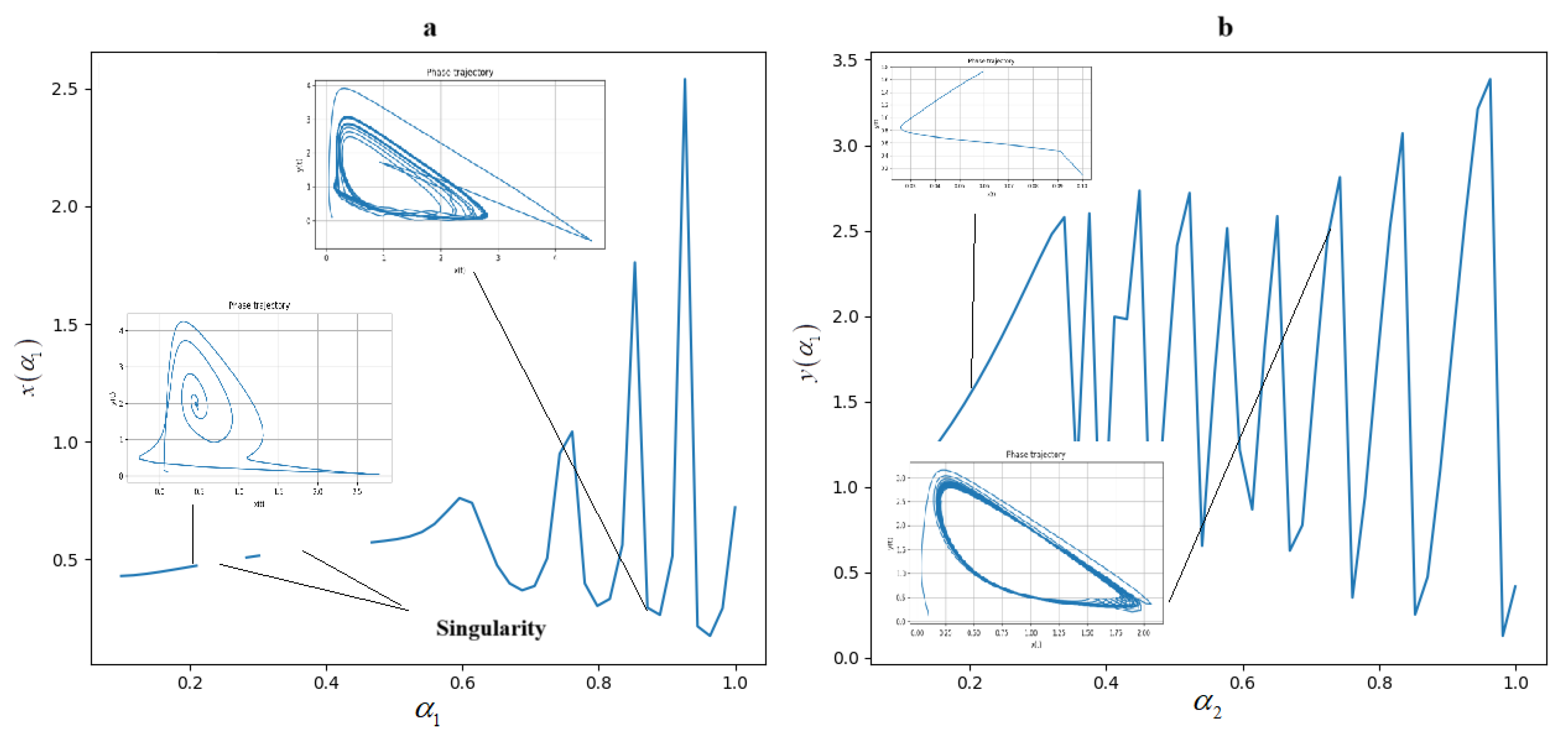
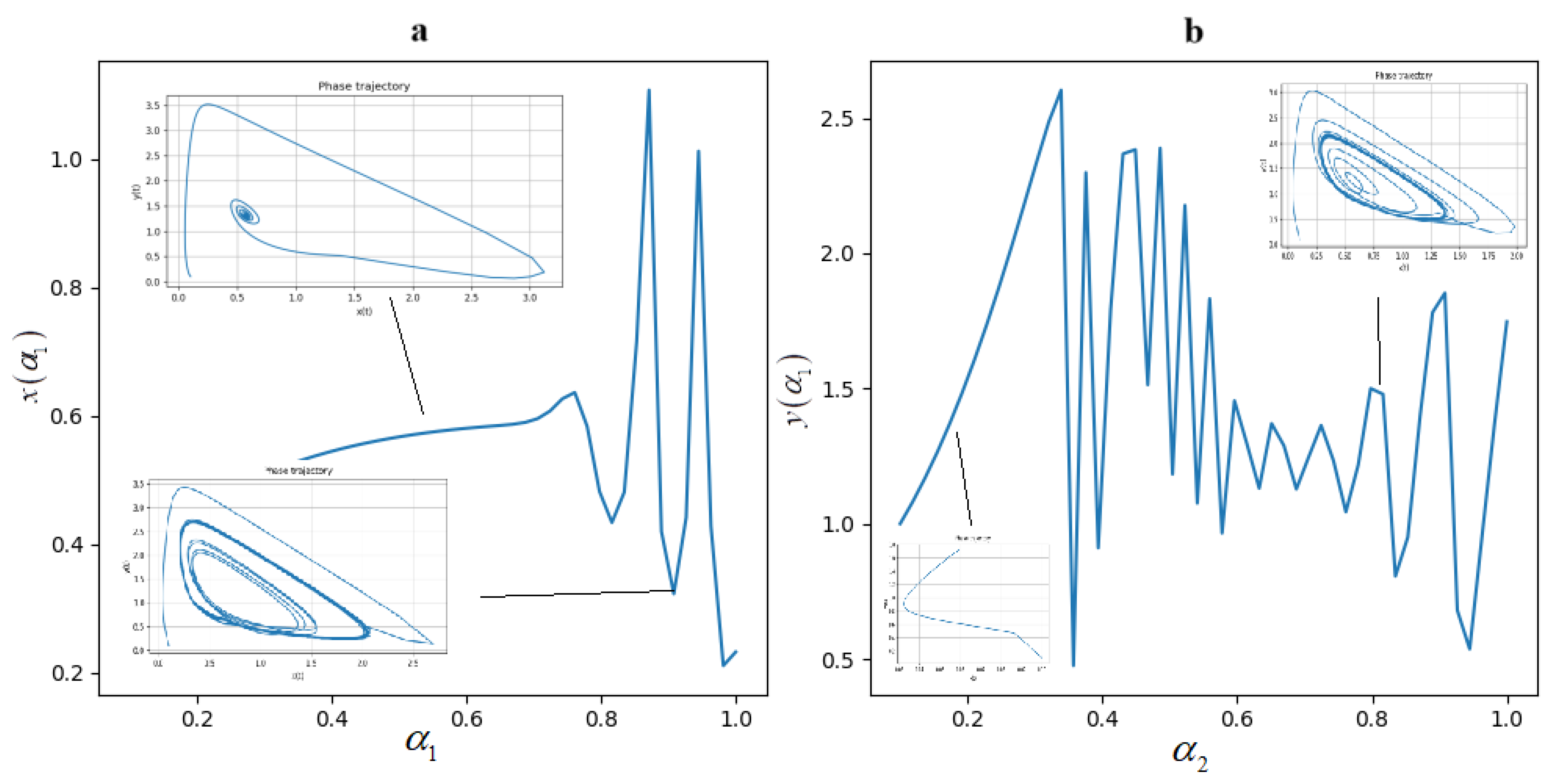
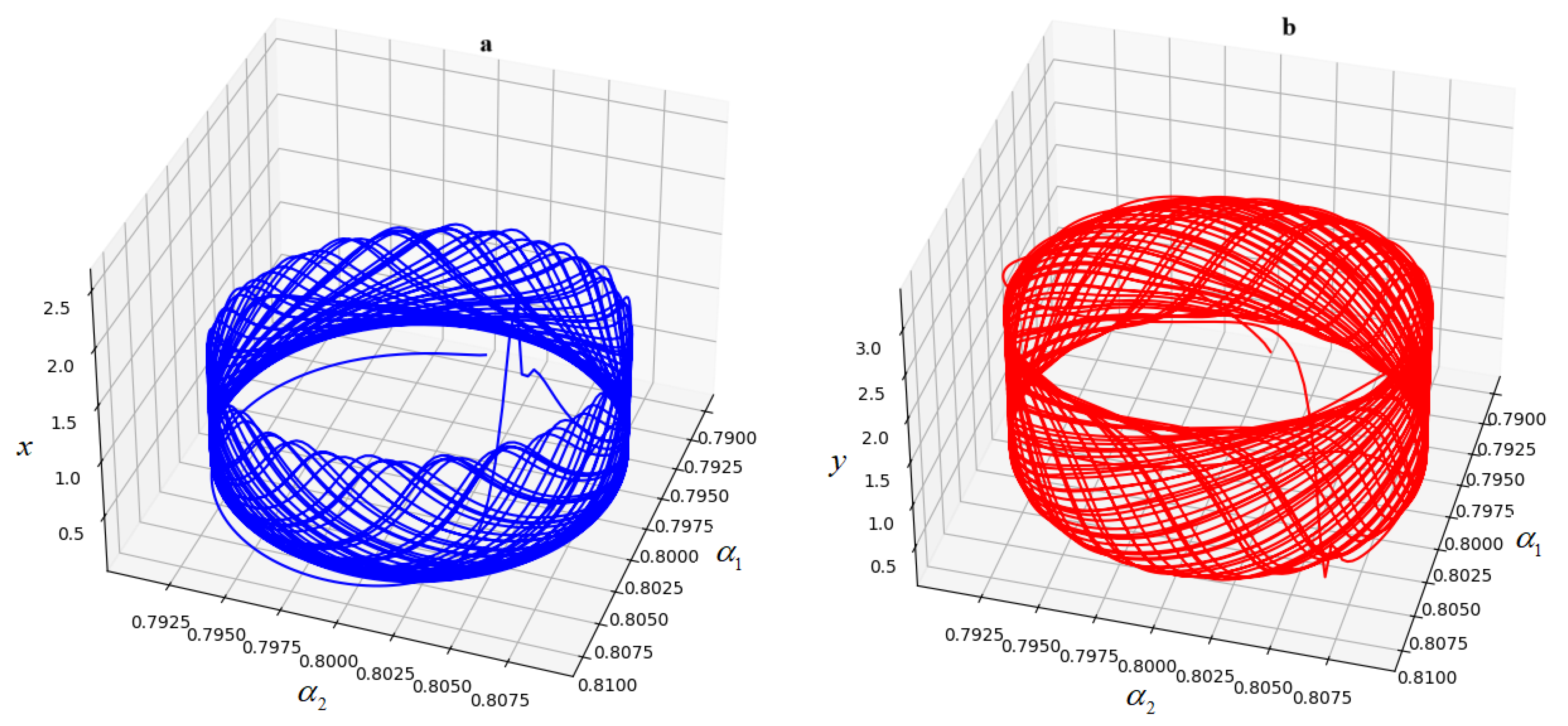
6. Bifurcation Diagrams

Definition 3. 
A bifurcation diagram is a graphical representation of changes in the structure of solutions of a dynamic system when the parameters change. It shows how the stable and unstable states of the system change depending on the values of the parameters.
Let us look at some examples of constructing bifurcation diagrams.
Example 1. 
Figure 3 shows a graph of 3D surfaces x α 1 , α 2 and y α 1 , α 2 , where α 1 , α 2 0.1 , 1 , v 0 = 0.6 , w 0 = 0.03 , h 0 = 1.3 , θ = 1 , x 0 = 0.1 , y 0 = 0.1 , t 0 , 100 , N = 3000 , α 1 , α 2 are constants.
Figure 3 shows bifurcation diagrams in the form of surfaces of the sought solution x and y from the values of the orders of fractional derivatives α 1 and α 2 . Note that on the surfaces of Figure 3a,b, there are regions that are responsible for regular modes; for example, damped oscillations correspond to regions without spikes, and in the region with spikes, limit cycles can form, as well as pre-chaotic or chaotic modes. In addition, we see a region of torn regions, which, as we will show later, is associated with singularity.
In Figure 4, a bifurcation diagram is given—a section of the surface in Figure 3 at α 2 = 1 for the solution x (Figure 4a) and at α 1 = 1 for the solution y (Figure 4b). We see three regimes in these bifurcation diagrams, for example, in Figure 4a: First, there is a decaying regime up to α 1 = 0.6 , and the dashed line at the beginning indicates a singularity. Then, there are bursts that indicate a limit cycle. Moreover, in Figure 4a, bursts with increasing amplitude indicate that the orbit of the limit cycle increases. This is confirmed by the phase trajectories in the insets of Figure 4a,b.
Figure 5 shows bifurcation diagrams constructed for other parameter values with insets of phase trajectories for different sections of the diagrams. Here, we can note, for example, that in Figure 5a, the bursts occur with decreasing amplitude, which indicates a decrease in the orbit of the limit cycle. There is no singularity here.
In Figure 5b, the bursts first occur with increasing amplitude, then with decreasing amplitude, etc. However, if such alternation is inconsistent or has a chaotic character, then we will arrive at chaotic or pre-chaotic regimes.
Note that in Figure 5b, we also see an aperiodic regime—a regime in which there are no oscillations, which corresponds to a curve without bursts on the bifurcation diagram.
Let us now consider another example of a fractional dynamical Selkov system, where α 1 t and α 2 t are functions of t.
Example 2. 
We will choose the following values of the parameters: N = 10000 ,   t 0 , 1000 ; the remaining parameters will be taken from Example 1. The orders of the fractional derivatives change in time t according to the following laws:
α 1 t = 0.8 1 100 cos 0.1 π t , α 2 t = 0.8 9 1000 sin 0.1 π t .
Let us construct bifurcation diagrams in the form of surfaces for solutions x α 1 , α 2 and y α 1 , α 2 (Figure 6).
We see that in Figure 6, the surfaces represent a completely regular cylindrical figure.
Figure 7 shows the calculated curves α 1 t and α 2 t obtained by Formula (4) (Figure 7a,b). Sections of the surface by planes x α 1 and y α 2 are shown in Figure 7c,d, as well as the phase trajectory in Figure 7e.
Here, we also see on the bifurcation diagrams (Figure 8) that there are “calm” sections, and there are sections with bursts. All this indicates the presence of different dynamic regimes.

7. Conclusions

A fractional dynamic Selkov system with non-constant coefficients is proposed, which is studied using the Adams–Bashforth–Multon numerical algorithm. The numerical algorithm is implemented in the ABMSelkovFracSim software package. The software package is written in the Python programming language in the PyCharm 2014.1 environment. Using the software package, calculations can be performed in two modes, when the orders of fractional derivatives and coefficients are constant and when they are functions of time. The simulation results can be displayed using graphs, which can also be saved for subsequent analysis. The calculation results themselves can be saved to a text file. Phase trajectories and oscillograms were obtained using the ABMSelkovFracSim software package.
Various bifurcation diagrams for the fractional dynamic Selkov system are studied in the case where θ = 1 . It is shown that the calculated curves of the dependences of the solution of the fractional dynamic Selkov system on the values of the orders of fractional derivatives characterize the change in dynamic modes, i.e., they are bifurcation diagrams. The presence of regular and chaotic modes, as well as the presence of singularity, is shown.
Further study of bifurcation diagrams is related to the construction of dynamic mode maps [23,24], as well as the case where θ 1 . For these purposes, it is necessary to involve more powerful computing resources, for example, computing servers with the ability to use CPU or GPU processors.
One of the further continuations of this research is the expansion of the functionality of the ABMSelkovFracSim software package. In particular, it is possible to provide the addition of modules for the qualitative analysis of the fractional dynamic Selkov system: construction of bifurcation diagrams, Test 0-1 [25,26], maximum Lyapunov exponents, etc.

Funding

The work was carried out within the framework of the state assignment of IKIR FEB RAS (reg. No. 124012300245-2), and the development of the ABMSelkovFracSim software package was financed by the Russian Science Foundation, No. 22-11-00064 (https://rscf.ru/en/project/22-11-00064/ accessed on 12 May 2022).

Data Availability Statement

The original contributions presented in this study are included in the article. Further inquiries can be directed to the corresponding author.

Conflicts of Interest

The author declares no conflicts of interest.

References

  1. Selkov, E.E. Self-oscillations in glycolysis. I. A simple kinetic model. Eur. J. Biochem. 1968, 4, 79–86. [Google Scholar] [CrossRef] [PubMed]
  2. Makovetsky, V.I.; Dudchenko, I.P.; Zakupin, A.S. Auto oscillation model of microseism’s sources. Geosist. Pereh. Zon. 2017, 4, 37–46. [Google Scholar]
  3. Parovik, R.; Rakhmonov, Z.; Zunnunov, R. Modeling of fracture concentration by Sel’kov fractional dynamic system. E3S Web Conf. EDP Sci. 2020, 196, 02018. [Google Scholar] [CrossRef]
  4. Parovik, R.I. Studies of the Fractional Selkov Dynamical System for Describing the Self-Oscillatory Regime of Microseisms. Mathematics 2022, 10, 4208. [Google Scholar] [CrossRef]
  5. Rabotnov, Y.N. Elements of Hereditary Solid Mechanics; Mir: Moscow, Russia, 1980; p. 387. [Google Scholar]
  6. Hoffmann, X.R.; Marián, B. Memory-induced complex contagion in epidemic spreading. New J. Phys. 2019, 21, 033034. [Google Scholar] [CrossRef]
  7. Tarasov, V.E. On history of mathematical economics: Application of fractional calculus. Mathematics 2019, 7, 509. [Google Scholar] [CrossRef]
  8. Volterra, V. Functional Theory, Integral and Integro-Differential Equations; Dover Publications: New York, NY, USA, 2005; p. 288. [Google Scholar]
  9. Nakhushev, A.M. Fractional Calculus and Its Applications; Fizmatlit: Moscow, Russia, 2003; p. 272. [Google Scholar]
  10. Kilbas, A.A.; Srivastava, H.M.; Trujillo, J.J. Theory and Applications of Fractional Differential Equations; Elsevier: Amsterdam, The Netherlands, 2006; Volume 204, p. 523. [Google Scholar]
  11. Parovik, R.I. Selkov Dynamic System with Variable Heredity for Describing Microseismic Regimes. In Solar-Terrestrial Relations and Physics of Earthquake Precursors: Proceedings of the XIII International Conference; Springer Nature Switzerland AG: Cham, Switzerland, 2023; pp. 166–178. [Google Scholar]
  12. Parovik, R.I. Qualitative analysis of Selkov’s fractional dynamical system with variable memory using a modified Test 0–1 algorithm. Vestn. KRAUNC. Fiz.-Mat. Nauki. 2023, 45, 9–23. [Google Scholar]
  13. Shaw, Z.A. Learn Python the Hard Way; Addison-Wesley Professional: New York, NY, USA, 2024; p. 306. [Google Scholar]
  14. Van Horn, B.M., II; Nguyen, Q. Hands-On Application Development with PyCharm: Build Applications Like a Pro with the Ultimate Python Development Tool; Packt Publishing Ltd.: Birmingham, UK, 2023; p. 652. [Google Scholar]
  15. Novozhenova, O.G. Life And Science of Alexey Gerasimov, One of the Pioneers of Fractional Calculus in Soviet Union. Fract. Calc. Appl. Anal. 2017, 20, 790–809. [Google Scholar] [CrossRef]
  16. Caputo, M.; Fabrizio, M. On the notion of fractional derivative and applications to the hysteresis phenomena. Meccanica 2017, 52, 3043–3052. [Google Scholar] [CrossRef]
  17. Aguilar, J.F.G.; Hernández, M.M. Space-Time Fractional Diffusion-Advection Equation with Caputo Derivative. Abstr. Appl. Anal. 2014, 2014, 283019. [Google Scholar] [CrossRef]
  18. Sun, H.; Chang, A.; Zhang, Y.; Chen, W. A Review on Variable-Order Fractional Differential Equations: Mathematical Foundations, Physical Models, Numerical Methods and Applications. Fract. Calc. Appl. Anal. 2019, 22, 27–59. [Google Scholar] [CrossRef]
  19. Patnaik, S.; Hollkamp, J.P.; Semperlotti, F. Applications of variable-order fractional operators: A review. Proc. R. Soc. A R. Soc. Publ. 2020, 476, 20190498. [Google Scholar] [CrossRef] [PubMed]
  20. Diethelm, K.; Ford, N.J.; Freed, A.D. A predictor-corrector approach for the numerical solution of fractional differential equations. Nonlinear Dyn. 2002, 29, 3–22. [Google Scholar] [CrossRef]
  21. Yang, C.; Liu, F. A computationally effective predictor-corrector method for simulating fractional order dynamical control system. ANZIAM J. 2005, 47, 168–184. [Google Scholar] [CrossRef]
  22. Garrappa, R. Numerical solution of fractional differential equations: A survey and a software tutorial. Mathematics 2018, 6, 016. [Google Scholar] [CrossRef]
  23. Bao, B.; Hu, J.; Cai, J.; Zhang, X.; Bao, H. Memristor-induced mode transitions and extreme multistability in a map-based neuron model. Nonlinear Dyn. 2023, 111, 3765–3779. [Google Scholar] [CrossRef]
  24. Colbrook, M.J.; Li, Q.; Raut, R.V.; Townsend, A. Beyond expectations: Residual dynamic mode decomposition and variance for stochastic dynamical systems. Nonlinear Dyn. 2024, 112, 2037–2061. [Google Scholar] [CrossRef]
  25. Gottwald, G.A.; Melbourne, I. On the implementation of the 0–1 test for chaos. SIAM J. Appl. Dyn. Syst. 2009, 8, 129–145. [Google Scholar] [CrossRef]
  26. Fouda, J.S.A.E.; Bodo, B.; Sabat, S.L.; Effa, J.Y.A. Modified 0–1 test for chaos detection in oversampled time series observations. Int. J. Bifurc. Chaos 2014, 24, 1450063. [Google Scholar] [CrossRef]
Figure 1. Interface of the software package ABMSelkovFracSim.
Mathematics 13 00372 g001
Figure 2. Calculation results: (a) α 1 = 0.8 ,   α 2 = 0.9 ,   θ = 1 [4]. (b) α 1 = 0.8 ,   α 2 = 0.9 ,   k 1 = 0.02 , k 2 = 0.01 ,   ϕ 1 = 3 ,   ϕ 2 = 1.5 ,   f 1 = 0.01 ,   f 2 = 0.03 ,   θ = 0.5 . (c) α 1 = 0.8 ,   α 2 = 0.9 ,   k 1 = 0.02 , k 2 = 0.01 ,   ϕ 1 = 3 ,   ϕ 2 = 1.5 ,   f 1 = 0.01 ,   f 2 = 0.03 ,   θ = 1.5 . (d) α 1 = 0.8 ,   α 2 = 0.9 ,   k 1 = 0.02 ,   k 2 = 0.01 , ϕ 1 = 3 ,   ϕ 2 = 1.5 ,   f 1 = 0.01 ,   f 2 = 0.03 ,   θ = 3 .
Mathematics 13 00372 g002
Figure 3. Surfaces: (a) x = x α 1 , α 2 ; (b) y = y α 1 , α 2 .
Mathematics 13 00372 g003
Figure 4. Calculated curves: (a) x α 1 , α 2 = 1 ; (b) y α 2 , α 1 = 1 .
Mathematics 13 00372 g004
Figure 5. Calculated curves: (a) x α 1 , α 2 = 0.8 ; (b) y α 2 , α 1 = 0.8 .
Mathematics 13 00372 g005
Figure 6. Three-dimensional surfaces: (a) x α 1 , α 2 ; (b) y α 1 , α 2 .
Mathematics 13 00372 g006
Figure 7. Calculated curves: (a) α 1 t ; (b) α 2 t ; (c) x α 1 ; (d) y α 2 ; (e) y = y x .
Mathematics 13 00372 g007
Figure 8. Bifurcation diagrams of the dependence of the solutions x and y on various values of the model parameters.
Mathematics 13 00372 g008
Disclaimer/Publisher’s Note: The statements, opinions and data contained in all publications are solely those of the individual author(s) and contributor(s) and not of MDPI and/or the editor(s). MDPI and/or the editor(s) disclaim responsibility for any injury to people or property resulting from any ideas, methods, instructions or products referred to in the content.

