
Variational Iteration and Linearized Liapunov Methods for Seeking the Analytic Solutions of Nonlinear Boundary Value Problems


Abstract
1. Introduction
2. The Existence of Solutions
2.1. Existence Theorem
2.2. Application to an Example
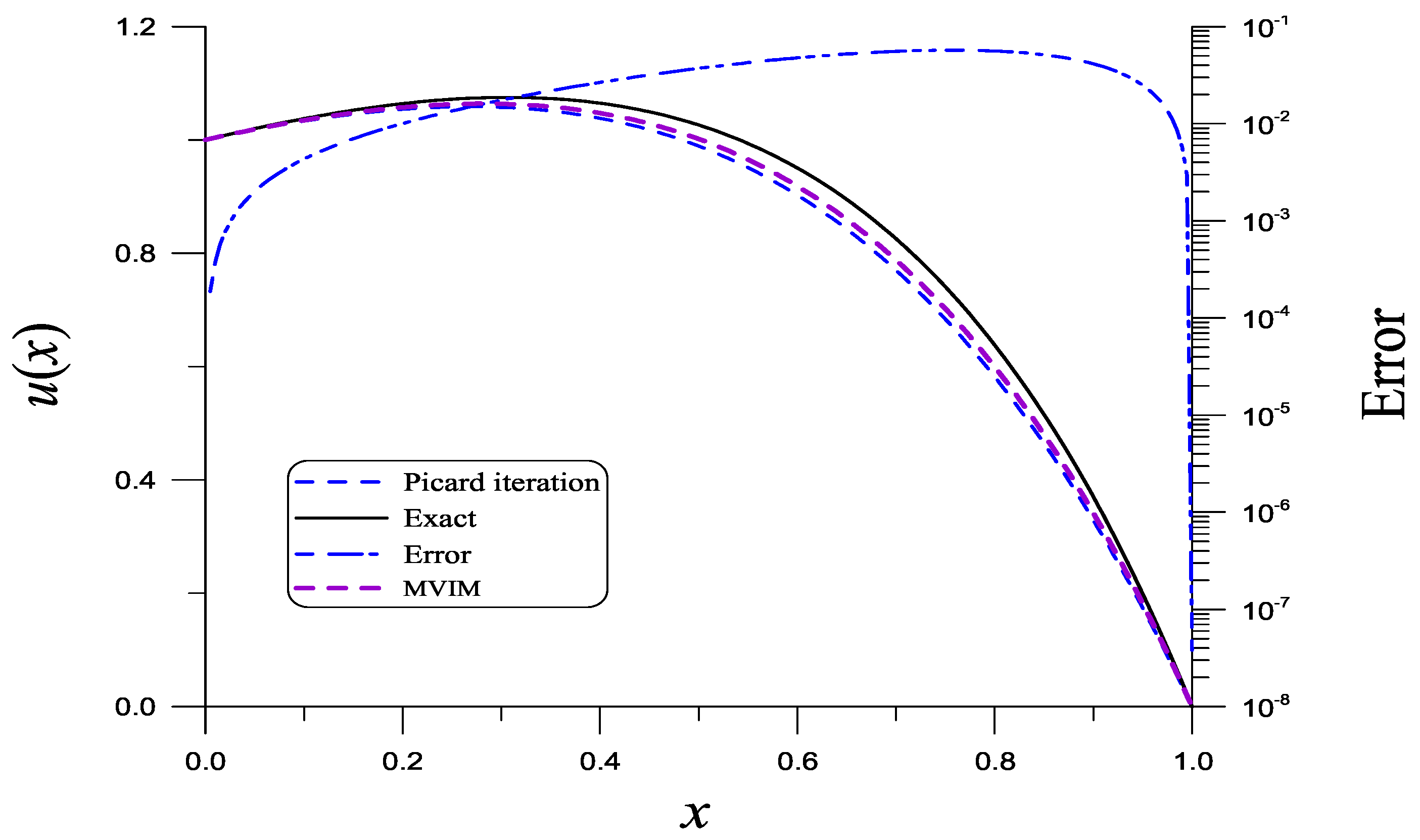
3. Slow Convergence of the Picard Iteration Method
4. Boundary Shape Function Method
5. A Modified Variational Iteration Method
5.1. Variational Iteration Method
5.2. A Modified VIM
5.3. Determination of the Right-Hand Values
5.4. Nonlocal Boundary Conditions
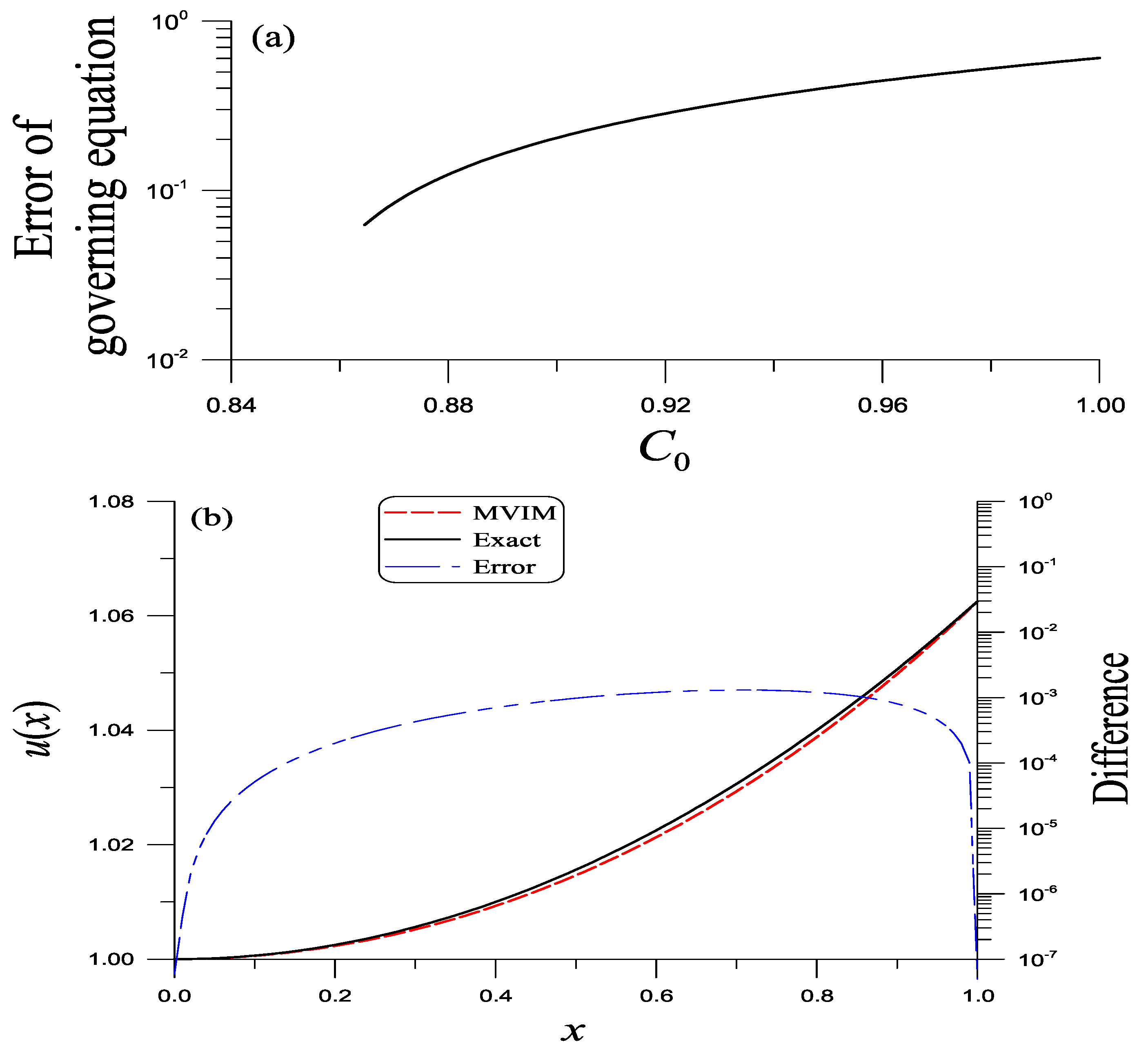
6. Example Testing for the MVIM
A Nonlocal BVP
7. Linearized Liapunov Method for Seeking Analytic Solutions
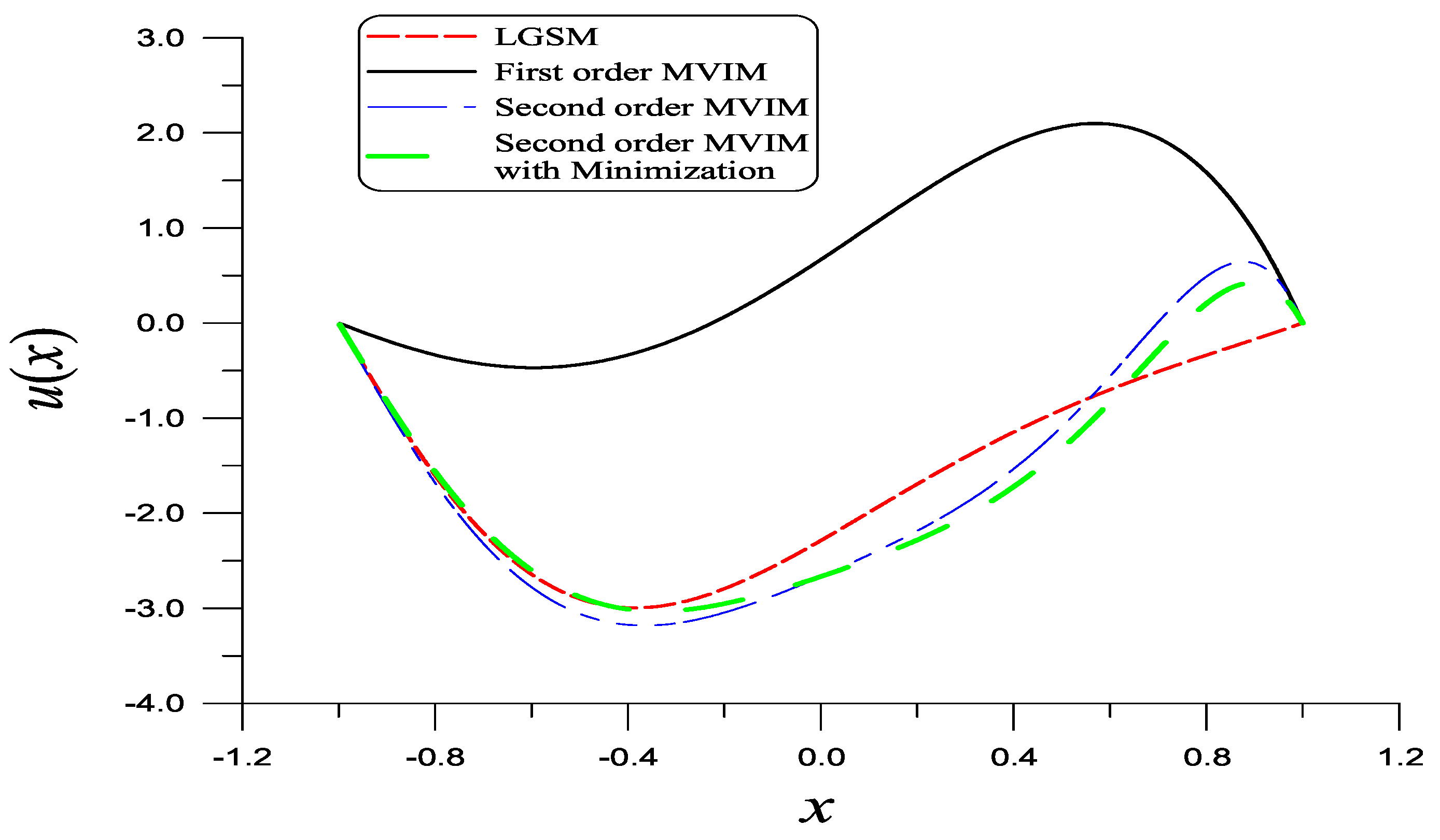
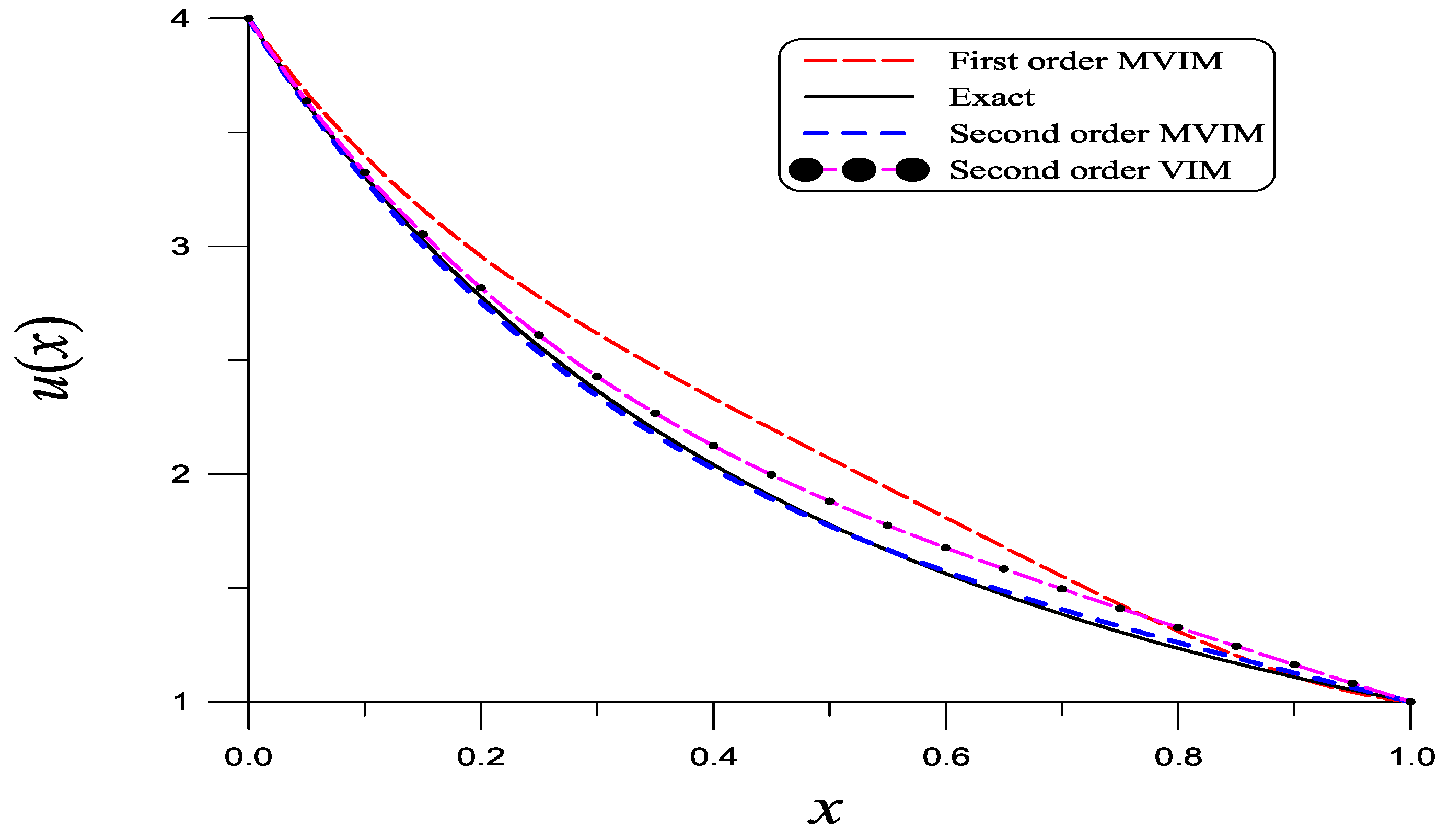
8. Examples Testing for the Linearized Liapunov Method
9. Conclusions
Author Contributions
Funding
Data Availability Statement
Conflicts of Interest
Appendix A

| x | Exact | Equation (A6) | Equation (A5) | Equation (A7) |
|---|---|---|---|---|
| 0 | 1.00000 | 1.00000 | 1.00000 | 1.00000 |
| 0.1 | 1.03753 | 1.05255 | 1.03468 | 1.03025 |
| 0.2 | 1.06402 | 1.08885 | 1.05740 | 1.04716 |
| 0.3 | 1.07501 | 1.10347 | 1.06351 | 1.04601 |
| 0.4 | 1.06482 | 1.09023 | 1.04724 | 1.02132 |
| 0.5 | 1.02626 | 1.04222 | 1.00164 | 0.966968 |
| 0.6 | 0.950319 | 0.951926 | 0.918457 | 0.876260 |
| 0.7 | 0.825678 | 0.811284 | 0.788167 | 0.741986 |
| 0.8 | 0.638204 | 0.611764 | 0.599927 | 0.556525 |
| 0.9 | 0.370281 | 0.344429 | 0.341633 | 0.311926 |
| 1.0 | 0 | 0 | 0 |
Appendix B
References
- Cash, J.R. On the numerical integration of nonlinear two-point boundary value problems using iterated deferred corrections, Part 1: A survey and comparison of some one-step formulae. Comput. Math. Appl. 1986, 12, 1029–1048. [Google Scholar] [CrossRef]
- Cash, J.R. On the numerical integration of nonlinear two-point boundary value problems using iterated deferred corrections, Part 2: The development and analysis of highly stable deferred correction formulae. SIAM J. Numer. Anal. 1988, 25, 862–882. [Google Scholar] [CrossRef]
- Cash, J.R.; Wright, R.W. Continuous extensions of deferred correction schemes for the numerical solution of nonlinear two-point boundary value problems. Appl. Numer. Math. 1998, 28, 227–244. [Google Scholar] [CrossRef]
- Ascher, U.M.; Mattheij, R.M.M.; Russell, R.D. Numerical Solution of Boundary Value Problems for Ordinary Differential Equations; SIAM: Philadelphia, PA, USA, 1995. [Google Scholar]
- Liu, C.S. The Lie-group shooting method for nonlinear two-point boundary value problems exhibiting multiple solutions. Comput. Model. Eng. Sci. 2006, 13, 149–163. [Google Scholar]
- Cabada, A.; Pouso, R.L. Existence theory for functional p-Laplacian equations with variable exponents. Nonlinear Anal. 2003, 52, 557–572. [Google Scholar] [CrossRef]
- Cabada, A.; O’Regan, D.; Pouso, R.L. Second order problems with functional conditions including Sturm-Liouville and multipoint conditions. Math. Nachr. 2008, 281, 1254–1263. [Google Scholar] [CrossRef]
- Mawhin, J.; Thompson, H.B. Bounding surfaces and second order quasilinear equations with compatible nonlinear functional boundary conditions. Adv. Nonlinear Stud. 2011, 11, 157–172. [Google Scholar] [CrossRef]
- Erbe, L.H. Nonlinear boundary value problems for second order differential equations. J. Diff. Equ. 1970, 7, 459–472. [Google Scholar] [CrossRef]
- Mawhin, J.; Schmitt, K. Upper and lower solutions and semilinear second order elliptic equations with non-linear boundary conditions. Proc. Roy. Soc. Edinburgh 1984, 97, 199–207. [Google Scholar] [CrossRef]
- De Coster, C.; Habets, P. Two-Point Boundary Value Problems: Lower And Upper Solutions; Elsevier: New York, NY, USA, 2006. [Google Scholar]
- He, J.H. Variational iteration method – a kind of non-linear analytical technique: Some examples. Int. J. Non-linear Mech. 1999, 34, 699–708. [Google Scholar] [CrossRef]
- He, J.H. Variational iteration method for autonomous ordinary systems. Appl. Math. Comput. 2000, 114, 115–123. [Google Scholar] [CrossRef]
- Herisanu, N.; Marinca, V. A modified variational iteration method for strongly nonlinear problems. Nonlinear Sci. Lett. A 2010, 1, 183–192. [Google Scholar]
- Turkyilmazoglu, M. An optimal variational iteration method. Appl. Math. Lett. 2011, 24, 762–765. [Google Scholar] [CrossRef]
- Wang, X.; Atluri, S.N. A unification of the concepts of the variational iteration, Adomian decomposition and Picard iteration methods; and a local variational iteration method. Comput. Model. Eng. Sci. 2016, 111, 567–585. [Google Scholar]
- Chang, S.H. Convergence of variational iteration method applied to two-point diffusion problems. Appl. Math. Model. 2016, 40, 6805–6810. [Google Scholar] [CrossRef]
- Chang, S.H. A variational iteration method involving Adomian polynomials for a strongly nonlinear boundary value problem. East Asian J. Appl. Math. 2019, 9, 153–164. [Google Scholar]
- Farkas, M. Periodic Motions; Springer: New York, NY, USA, 1994. [Google Scholar]
- Liapunov, A.M. Sur une série dans la théorie des équations différentielles linéaires du second ordre à coefficients périodiques. Zap. Akad. Nauk Fiz.-Mat. Otd. 8th series 1902, 13, 1–70. [Google Scholar]
- He, J.H. Homotopy perturbation method: A new nonlinear analytical technique. Appl. Math. Comput. 2003, 135, 73–79. [Google Scholar] [CrossRef]
- He, J.H. Homotopy perturbation method for solving boundary value problems. Phy. Lett. A 2006, 350, 87–88. [Google Scholar] [CrossRef]
- Noor, M.A.; Mohyud-Din, S.T. Homotopy perturbation method for solving sixth-order boundary value problems. Comput. Math. Appl. 2008, 55, 2953–2972. [Google Scholar] [CrossRef]
- Chun, C.; Sakthivel, R. Homotopy perturbation technique for solving two-point boundary value problems–comparison with other methods. Comput. Phy. Communi. 2010, 181, 1021–1024. [Google Scholar] [CrossRef]
- Khuri, S.A.; Sayfy, A. Generalizing the variational iteration method for BVPs: Proper setting of the correction functional. Appl. Math. Lett. 2017, 68, 68–75. [Google Scholar] [CrossRef]
- Liu, C.S.; Chang, C.W. Boundary shape function method for nonlinear BVP, automatically satisfying prescribed multipoint boundary conditions. Bound. Value Prob. 2020, 2020, 139. [Google Scholar] [CrossRef]
- Coddington, E.A.; Levinson, N. Theory of Ordinary Differential Equations; McGraw-Hill: New York, NY, USA, 1955. [Google Scholar]
- Reid, W.T. Ordinary Differential Equations; John Wiley & Son: New York, NY, USA, 1971. [Google Scholar]
- Zhou, Z.; Shen, J. A second-order boundary value problem with nonlinear and mixed boundary conditions: Existence, uniqueness, and approximation. Abstr. Appl. Anal. 2010, 2010, 287473. [Google Scholar] [CrossRef]
- Liu, C.S.; Chang, J.R. Boundary shape functions methods for solving the nonlinear singularly perturbed problems with Robin boundary conditions. Int. J. Nonlinear Sci. Numer. Simul. 2020, 21, 797–806. [Google Scholar] [CrossRef]
- Rani, G.S.; Jayan, S.; Nagaraja, K.V. An extension of golden section algorithm for n-variable functions with MATLAB code. IOP Conf. Ser. Mater. Sci. Eng. 2018, 577, 012175. [Google Scholar] [CrossRef]
- Lu, J. Variational iteration method for solving two-point boundary value problems. J. Comput. Appl. Math. 2007, 207, 92–95. [Google Scholar] [CrossRef]
- Adomian, G.; Elrod, M.; Rach, R. A new approach to boundary value equations and application to a generalization of Airy’s equation. J. Math. Anal. Appl. 1989, 140, 554–568. [Google Scholar] [CrossRef]
- Ha, S.N. A nonlinear shooting method for two-point boundary value problems. Comput. Math. Appl. 2001, 42, 1411–1420. [Google Scholar] [CrossRef]
- Ha, S.N.; Lee, C.R. Numerical study for two-point boundary value problems using Green’s functions. Comput. Math. Appl. 2002, 44, 1599–1608. [Google Scholar] [CrossRef]
- Liu, C.S.; Kuo, C.L.; Chang, C.W. Decomposition-linearization-sequential homotopy methods for nonlinear differential/integral equations. Mathematics 2024, 12, 3557. [Google Scholar] [CrossRef]
- Liu, C.S.; Chang, C.W. Lie-group shooting/boundary shape function methods for solving nonlinear boundary value problems. Symmetry 2022, 14, 778. [Google Scholar] [CrossRef]
- Chang, C.W.; Chang, J.R.; Liu, C.S. The Lie-group shooting method for solving classical Blasius flat-plate problem. Comput. Mater. Contin. 2008, 7, 139–153. [Google Scholar]
- Cortell, R. Numerical solutions of the classical Blasius flat-plate problem. Appl. Math. Comput. 2005, 170, 706–710. [Google Scholar] [CrossRef]
- Zheng, L.C.; Chen, X.H.; Chang, X.X. Analytical approximants for a boundary layer flow on a stretching moving surface with a power velocity. Int. J. Appl. Mech. Eng. 2004, 9, 795–802. [Google Scholar]
- Khuri, S.A.; Sayfy, A. Self-adjoint singularly perturbed boundary value problems: An adaptive variational approach. Math. Meth. Appl. Sci. 2013, 36, 1070–1079. [Google Scholar] [CrossRef]


| x | Exact | Present | Lu [32] |
|---|---|---|---|
| 0 | 1.00000 | 1.00000 | 0.8646 |
| 0.1 | 1.00063 | 1.00057 | 0.8665 |
| 0.2 | 1.00250 | 100230 | 0.8723 |
| 0.3 | 1.00563 | 1.00520 | 0.8820 |
| 0.4 | 1.01000 | 1.00930 | 0.8956 |
| 0.5 | 1.01563 | 1.01465 | 0.9131 |
| 0.6 | 1.02250 | 1.02130 | 0.9346 |
| 0.7 | 1.03062 | 1.02932 | 0.9603 |
| 0.8 | 1.04000 | 1.03880 | 0.9901 |
| 0.9 | 1.05062 | 1.04982 | 1.0241 |
| 1.0 | 1.06250 | 1.06250 | 1.0625 |
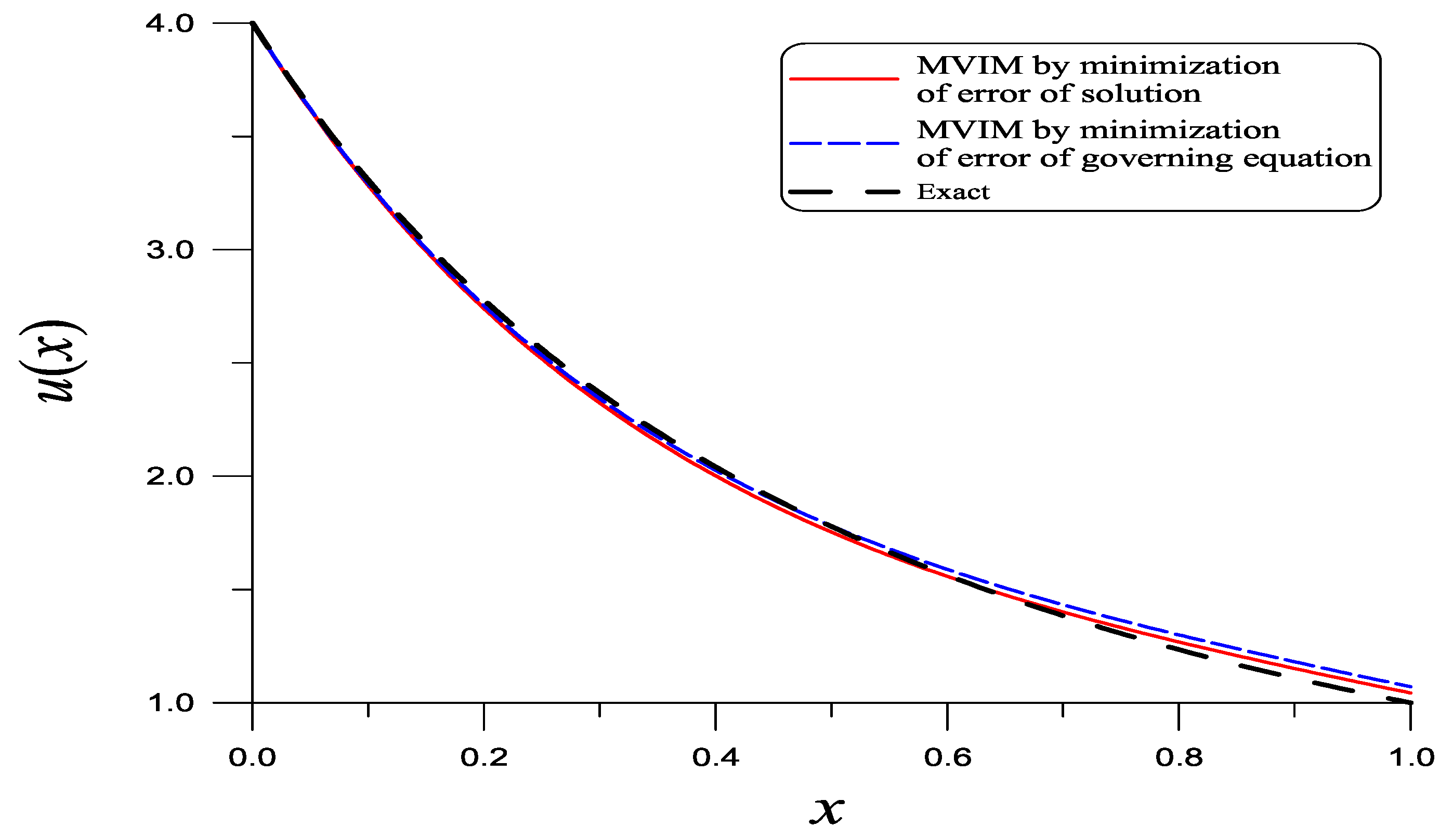
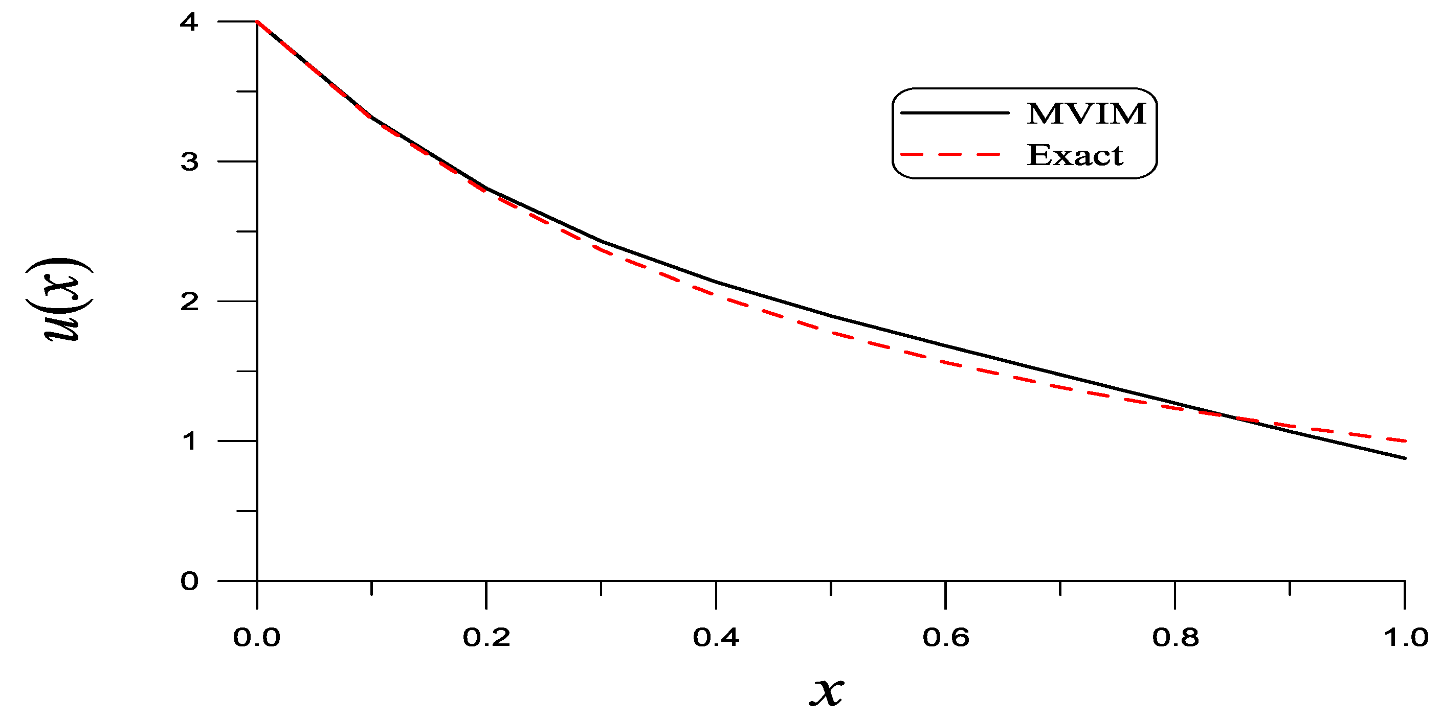
| x | Exact | Present | Absolute Error |
|---|---|---|---|
| 0 | 4.0000 | 4.0000 | 0.0 |
| 0.1 | 3.3058 | 3.3135 | 0.0077 |
| 0.2 | 2.7778 | 2.8073 | 0.0295 |
| 0.3 | 2.3669 | 2.4295 | 0.0626 |
| 0.4 | 2.0408 | 2.1372 | 0.1964 |
| 0.5 | 1.7778 | 1.8961 | 0.1183 |
| 0.6 | 1.5625 | 1.6810 | 0.1185 |
| 0.7 | 1.3841 | 1.4751 | 0.0910 |
| 0.8 | 1.2346 | 1.2706 | 0.0360 |
| 0.9 | 1.1080 | 1.0685 | 0.0395 |
| 1.0 | 1.0000 | 0.8785 | 0.1215 |
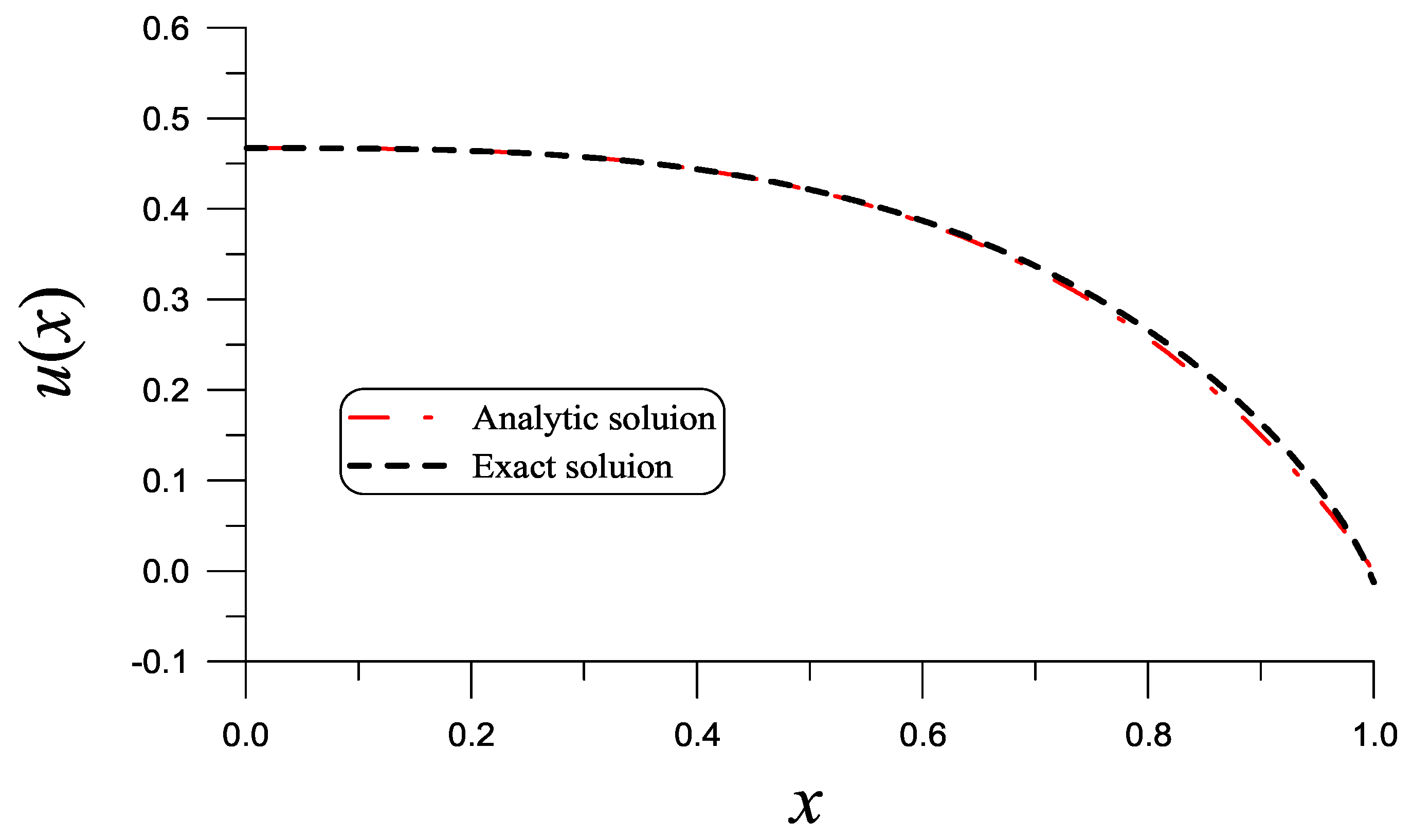
| x | Equation (115) | Equation (116) | Exact | Equation (125) |
|---|---|---|---|---|
| 0.1 | −0.658247 | −0.654982 | −0.654333 | −0.826110 |
| 0.2 | −0.481409 | −0.479186 | −0.478722 | −0.600393 |
| 0.4 | −0.118469 | −0.119156 | −0.119050 | −0.136309 |
| 0.5 | 0.064340 | 0.061822 | 0.061794 | 0.095388 |
| 0.7 | 0.430574 | 0.424832 | 0.424726 | 0.540575 |
| 0.9 | 0.804495 | 0.799604 | 0.799879 | 0.902546 |
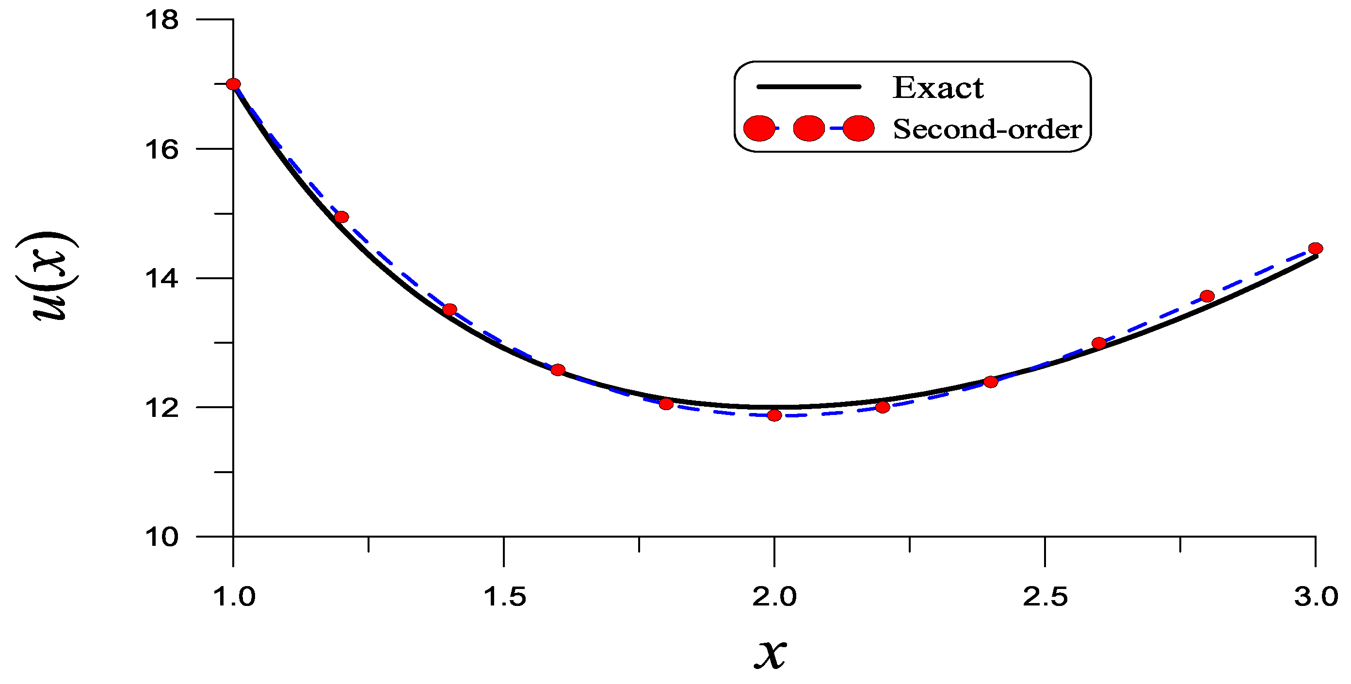
| x | 1.1 | 1.4 | 1.8 | 2.0 | 2.4 | 2.7 | 3 |
| Exact | 15.755 | 13.389 | 12.129 | 12 | 12.427 | 13.216 | 14.333 |
| Present | 15.883 | 13.513 | 12.053 | 11.875 | 12.394 | 13.346 | 14.458 |
| RE |
Disclaimer/Publisher’s Note: The statements, opinions and data contained in all publications are solely those of the individual author(s) and contributor(s) and not of MDPI and/or the editor(s). MDPI and/or the editor(s) disclaim responsibility for any injury to people or property resulting from any ideas, methods, instructions or products referred to in the content. |
© 2025 by the authors. Licensee MDPI, Basel, Switzerland. This article is an open access article distributed under the terms and conditions of the Creative Commons Attribution (CC BY) license (https://creativecommons.org/licenses/by/4.0/).
Share and Cite
Liu, C.-S.; Li, B.; Kuo, C.-L. Variational Iteration and Linearized Liapunov Methods for Seeking the Analytic Solutions of Nonlinear Boundary Value Problems. Mathematics 2025, 13, 354. https://doi.org/10.3390/math13030354
Liu C-S, Li B, Kuo C-L. Variational Iteration and Linearized Liapunov Methods for Seeking the Analytic Solutions of Nonlinear Boundary Value Problems. Mathematics. 2025; 13(3):354. https://doi.org/10.3390/math13030354
Chicago/Turabian StyleLiu, Chein-Shan, Botong Li, and Chung-Lun Kuo. 2025. "Variational Iteration and Linearized Liapunov Methods for Seeking the Analytic Solutions of Nonlinear Boundary Value Problems" Mathematics 13, no. 3: 354. https://doi.org/10.3390/math13030354
APA StyleLiu, C.-S., Li, B., & Kuo, C.-L. (2025). Variational Iteration and Linearized Liapunov Methods for Seeking the Analytic Solutions of Nonlinear Boundary Value Problems. Mathematics, 13(3), 354. https://doi.org/10.3390/math13030354