Machine Learning Tool for Analyzing Finite Buffer Queueing Systems

Abstract

Queueing delays are one very important performance measure for most engineering network systems. Providing low-delay systems is a major goal of service providers, as it is a leading concern for users/customers. These network systems and their performance measures are typically analyzed using queueing-based models. Even though there are several available strong and precise mathematical models for analyzing queueing systems, their applications are limited to simple and small-scale systems due to their lack of scalability in real-life systems. Researchers have spent a good portion of their efforts toward perfecting the analysis of such systems. Precise and accurate results are available for single-node systems with standard operations. However, for analyzing multi-node systems with complex operations, one has to resort to approximations or simulations. Some of these approximations usually give an oversimplified view of such systems; these approximations remain quite limited. In this paper, we present a machine learning tool that can potentially be used to analyze most finite buffer queues to obtain reasonable approximations for the mean number of items in such systems. The machine learning tool we develop is based on supervised learning using the Michaelis–Menten non-linear model used in biochemistry and the results are simple to obtain. It is fast and very scalable; these characteristics represent the main features of this approach compared to existing systems. The coefficient of determination $R^2$ for all the examples presented are all higher than $90\%$, with some as high as $99.6\%$.

1. Introduction

Many of our day-to-day activities depend considerably on communication systems, specifically on communications and computer networks that carry and deliver messages between humans, devices, etc. One of the most important performance measures for these systems as perceived by users and service providers is latency, along with reliability and other types of measures. Therefore, it is extremely relevant that service providers are able to reasonably assess and measure such delays. Even though delay is the intended measure that is required for analysis, the number of items waiting in the queue is often used as a pseudo for estimating delay. Service providers need to develop tools for estimating delays and/or the number of items in a system for communication networks that are in use today. Similar to communications systems, transportation systems and manufacturing systems also need the same type of performance measures, making them extremely important in nearly all types of networks. The key methods for estimating delays in network systems are analytical queueing models and simulation tools, with the former being accepted as more precise and reliable when they can be used/developed.

Queueing theory [1] continues to be widely applied for modeling and analyzing the performance of systems with limited resources that offer services to entities with the possibility of queueing service requests. System evaluation is often conducted using either an analytical model or a simulation, with each of the two methods having their merits and limitations. In this paper, our goal is to offer a different, modest, and practical alternative to using analytical modeling or simulations in relation to queueing systems. The aim is to obtain very good estimates of the mean number in such systems, or the mean queue length, by using supervised machine learning. We present a machine learning tool that can be used to analyze most single-node and finite-buffer queues to obtain reasonable approximations for their mean queue lengths. The proposed tool will not have any restrictions on buffer size, except its being finite, and no restrictions on the traffic intensity. The results are further extended to multi-node systems, specifically to tandem queues, and later to tandem queueing systems with feedback.

One may ask why there is need to consider a machine learning tool for analyzing queueing systems, given the extensive literature on the subject. Even though there has been extensive and excellent work already carried out on queueing theory spanning over several years, there has been a nagging issue regarding scalability for real-life, large-size problems. Efforts have been carried out on different levels and directions to deal with handling practical queueing problems; however, scalability has been a persistent problem with the tools developed. In order to bring this matter to the forefront of this work, we discuss relevant background and related works pertaining to queueing theory in Section 2. This will assist in highlighting the excellent work that has been carried out in this field and how the issue of scalability is still of concern. This is why we consider machine learning a tool for handling scalability issues associated with queueing theory. The current paper is an initial attempt to show that machine learning has potential for being used for analyzing queueing theory, and to discuss future work pertaining to applications to large problems, hence pointing out how promising the tool is.

For the machine learning component, we assume the use of non-linear regression models in supervised learning tools and apply the non-linear Michaelis–Menten equation [2] for analyzing the behavior of M/M/c/K systems for any c and K, which is a well-studied model in the literature—further, exact results for its mean queue length are well known. We further show that the application of the proposed supervised learning tool can be extended to other and complex systems such as PH/PH/1/K systems and tandem systems with feedback. Our results are strictly focused on both proposing and demonstrating the merits of employing the non-linear regression model in supervise learning for estimating mean queue lengths in such systems. Issues in performance due to data size, integrity, and overfitting are not examined in this work. Such issues are common when using machine learning tools and are strongly related to the nature of the data and their application. Selecting a dataset for demonstrating the proposed solution’s performance under such issues can lead to certain biases that we intend to avoid; instead, we thus focus on the feasibility and simplicity of the proposed technique.

In this work, we limit our analysis to cases of systems with Markovian behaviors and stationary traffic intensities. While our selection of different types of queueing systems and networks is not exhaustive, we believe it is sufficient to demonstrate our proposed solution’s potential to deal with a significant number of different systems in both a simple and scalable manner. Other and more complex systems will be examined in our future work. The proposed solution, if deemed effective, can be applied to estimate in a timely and efficient manner mean queue lengths that are necessary in a variety of applications such as lane traffic scheduling [3], queue length estimations in signalized intersections [4], scheduling departures in busy airports [5], scheduling and prioritizing patient service in emergency care hospitals [6], scheduling network resources for delay sensitive applications [7], fair resource allocation in wireless networks [8], and many more other applications.

After covering the essential background on the topic, we present an overview of M/M/c/K systems with well-known closed form solutions for the queue lengths and waiting times, and develop a machine learning (ML) tool based on the supervised learning approach for analyzing the mean number in the queue. For the ML tool, we propose applying the Michaelis–Menten equation [2] for kinetics in biochemistry to represent the mean number in the system and an approach for finding the relevant parameters. We observe that the pattern of this system is the same for PH/PH/1/K systems and conjecture that the pattern observed follows for the GI/G/1/K systems. Even though the single-node results would go a long way to estimate the performance measure of interest very quickly for single-node systems, we believe that for the results to be fully appreciated, the idea should be extended to tandem queues, converging queues, and diverging queues. We explore the case of two queues in tandem as well as a network of four queues with feedback in this paper and defer the cases of converging and diverging systems to future works.

2. Background and Related Works

2.1. Overview of Queueing Analysis

Extensive research has been carried out over the years in queueing theory and for more than a century since Erlang, the Danish engineer/mathematician who made the field popular for telephony traffic in 1909. For more detailed information on Erlang’s work, see Brockmeyer and Halstrøm [9]. Since then, there have been continuous efforts by engineers, computer scientists, mathematicians, and operations research analysts to advance the theory and its applications. Even though significant progress has been made in this field, surprisingly, its applications, up to the early 1970s, were limited to very simple systems due to lack of scalability in real-life applications. In very seminal papers by Saaty [10] and Bhat [11], the authors pointed out the continuous growth of research papers in queueing and discussed how practitioners felt they could not use most of them, even though mathematicians felt the field had been well studied and there were several results available at the time. The problem was that what practitioners and theoretical researchers saw as usable results were divergent. There were at least two issues that needed to be addressed by researchers in the field of queueing theory at that time for results to be very useful to practitioners. One of them was that more realistic systems needed to be modeled, and the other was that the mathematical models should lend themselves to be computationally feasible for practitioners to compute measures for design purposes, rather than being left in the form of transforms, especially Laplace transforms.

In 1978, Jack Byrd [12] questioned why there were so few implementations of queueing theory, and went further to present some short case studies based on every day real-life systems for which effective solutions could not be obtained at the time. Several queueing theorists challenged this observation, including Narayan Bhat [13], pointing out that the problems considered were not true representations of queueing systems. Several researchers in the field took note. One of the key issues that queueing theory was facing at that time was that most results were in the form of Laplace transforms, and inverting those transforms was a numerical challenge. Efforts were devoted to developing transform inversions for some classes of queueing models or developing non-transform-based queueing algorithms.

As a result, Marcel Neuts along with a team of researchers decided to focus on developing queueing results that could be reasonably computed by practitioners. A series of papers on those methods include ([14,15,16,17,18]). These papers encouraged other mathematical researchers in the field to pursue computationally feasible tools for queueing analysis. Neuts [19] later advanced the theory of matrix geometric methods for practically analyzing a particular class of queues (the GI/M/1 types), which was later followed by Neuts [20] dealing with another important class of queues (the M/G/1 types). These were great advances in the field, later named Matrix-Analytic Methods (MAMs). However, there was still a major gap between theory and applications. Even though MAMs showed major promise in this area of obtaining numerical results for queueing models, there were still some challenges.

In the MAMs field, obtaining numerical results required computing some of the key matrices, such as the R and G matrices. Both matrices require significant effort to compute. Several other papers followed 30 years after Neuts’ work, with very deep theories emerging, but with limited advancement in real applications. Most of them are based on trying to model very complicated arrival and service processes, improving the computational efficiencies of existing exact methods such as those for computing R and G. The models developed, and often used, are limited not by the existing results but instead by scalability issues. For example, most of the queueing systems encountered in real life are finite buffer types, usually with very large buffer sizes, and traffic intensities larger than one. Even though finite buffer queues should be reasonably feasible to study and analyze, the Markov chains representing such systems have huge dimensions, making them practically inconvenient to analyze. Researchers often resort to approximating such queueing systems as infinite buffer queues and explore the use of mathematical tools that make such infinite buffer systems easier to analyze, thereby limiting their application to real life cases.

In an attempt to provide results based on transforms, considerable efforts were expended by other researchers in trying to develop efficient and effective tools for inverting transforms for practitioners. These efforts focused on developing numerical approaches for inverting the Laplace transforms and probability generating functions associated with queueing model results developed by mathematicians. Obtaining efficient and effective techniques for the inversions was thought to be key for exploring the transform-based results. Ward Whitt and several colleagues made significant progress in this area. A few examples of their work include ([21,22,23]), among a series of their works. They made some major progress in this area, but applications of the results still had scalability issues.

Another approach that received good attention was the fluid modeling approach based on a popular paper by Anick et al. [24]. Later, Ramaswami [25] worked on connecting fluid models with MAMs for studying queueing systems. The approach was well developed, but was also limited in terms of scalability.

From a scalability perspective, Whitt [26] made significant progress in making queueing theory accessible to practitioners dealing with network of queues. Specifically, Whitt developed the Queueing Network Analyzer (QNA), which succeeded in dealing with a class of queueing networks encountered in communications and industrial engineering. The QNA was well utilized, but was still limited in terms of scalability by modern-day network systems and requirements.

2.2. The Issue of Scalability

Engineers and mathematicians have spent a significant amount of research effort perfecting the analysis of such systems. Most of the advancements have been in dealing with more complicated real-life systems and developing computationally efficient methods for their analysis. Nevertheless, despite the major progress and success, the issue of scalability still persists, considering that most queueing models are usually only a component of a given large-scale model of interest for the practitioner. The practitioner usually wants to optimize some components of the queueing system; hence, performance measures of the queueing system are usually an input to a major complex analysis. Therefore, scalability issues need to be tackled.

Precise and accurate results are available for single-node systems with standard operations, with an infinite buffer as an example. So, most systems are approximated by such models. The problem with such approximations or representations is that the results are limited to systems that are stable, i.e., with traffic intensity less than one. Such infinite buffer queues with traffic intensities less than one are few and far between in real-life situations. Most service systems deal with traffic intensities greater than one—otherwise, the service providers would not find them economically feasible—and given the nature of the systems, the buffer sizes are finite and huge. In addition, most real-life systems, especially in communication networks, involve a series and networks of queues. Once we have to analyze these types of multi-node systems with complex operations, one has to resort to approximations or simulations. Some of these approximations usually give an oversimplified view of the system.

Our observation is that there are significant, exceptional, general, and well-refined mathematical and computationally based results that are currently available for queueing systems based on the excellent works of researchers in the field. However, the problem of their limited scalability remains. If the existing results discussed in the last few paragraphs can be harnessed with machine learning, then scalable results can potentially be developed, which is the main focus of this work.

2.3. The Case for Machine Learning

The idea of using machine learning to analyze queueing systems was suggested by Khoshnevis and Parisy [27] way back in 1993, when they showed that machine learning algorithms have a potential application, specifically in simulation stages of modeling. They demonstrated a sample application in simulations of queueing, and this showed some promise. Recently, the concept of applying machine learning to queueing systems has been gaining some traction due to the needs of more practical uses of queueing models. Chen and Yen [28] considered using machine learning to analyze multi-queue message scheduling in a specific controller and for a specific case of a controller area network. They used what they call a Type I and Type II machine learning approach for managing the variations in the queue load. Their method involved a hybrid learning approach for constructing the queueing model without the need for specifying the details of the model. However, their approach was limited to the scope covered in their application and the queueing model information was developed from simulations. Wartelle et al. [29] proposed a technique that utilizes queueing analysis and machine learning for forecasting and optimizing the performance of a system. Their result was developed for a specific application, namely, an emergency department. However, their method still required developing the specific details of the queueing model, which can become mathematically intractable when considering a larger scale of the system. Ojeda et al. [30] developed a data-driven approach called Deep Generative Service Times for learning the service and response time model in a queueing system. Their proposed method avoids the restriction of imposing explicit distribution forms in their analysis, but is limited to employing machine learning algorithms to certain parts of the queueing analysis.

Vishnevsky and Gorbunova [31] mentioned in their work that machine learning is highly effective based on their initial studies and suggested that it is an area that shows promise for further research. They further suggested that this area could lead to a new approach in the field of solving complex problems in the theory of queues, which is a very encouraging opinion. These viewpoints are further supported by Chocron et al. [32], who investigated under what regimes machine learning prediction is better than analytical queueing models. They observed that machine learning may outperform queueing models with high priority. The word “better” is subjective in this case as theoretical queueing models provide some form of precise results, with lots of computational effort, while machine learning provides much less precise results (good approximations) with much lower computational effort. Their work was based on a specific case study.

In another work, Sherzer et al. [33] examined how well machine learning can solve problems in queueing theory. They applied deep learning for evaluating the queue length in the M/G/1 system, which was later reduced to the M/PH/1 system. They used n moments of service to represent the PH (Phase–Type distribution). Their overall approach is as involved as standard queueing theory analytical models. However, they were able to demonstrate the ability for machine learning to analyze queueing problems. They later followed their study with another work reported in [34]. Kyritsis and Deriaz [35] explored how industries that use queueing tools can benefit from using machine learning to predict waiting times. They considered bank queues, and used a fully connected neural network model. They showed that the use of machine learning is promising as an alternative to analytical queueing models. Given how the use of machine learning for analyzing queue systems has been gaining traction lately, we further explore it with a different approach and focus on more generic cases rather than specific application-oriented cases.

3. The Michaelis–Menten Model

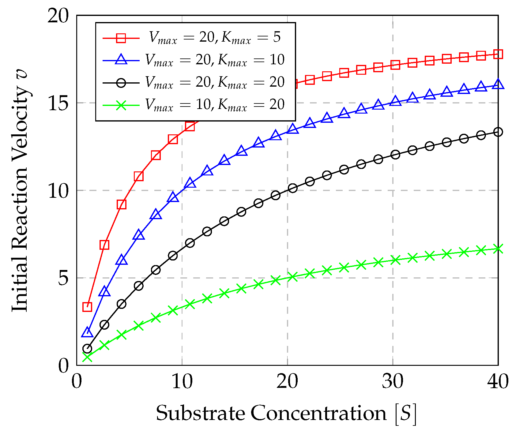
We first present the details of the Michaelis–Menten model [2]. The Michaelis-Menten (M-M) graph is a model used for enzyme kinetics in biochemistry. The M-M equation is of the form

$$v=V_{max}{\displaystyle \frac{\left[S\right]}{K_{max}+\left[S\right]}},$$

(1)

where the aim is to find, through a non-linear regression model, the parameter $V_{max}$, the maximum initial velocity, and the constant $K_{max}$, i.e., the parameters of the M-M equation which correspond to the observed substrate concentration $\left[S\right]$ (independent variable), and the velocity of reaction v, which is the dependent variable. The graphs in Figure 1 provide some numerical examples that illustrate the general behavior of the M-M model. Note that Equation (1) in a graphical form has a pattern which suggests that

$${\displaystyle \frac{dv}{d\left[S\right]}}\ge 0,\mathrm{and}{\displaystyle \frac{d^{2}v}{d{\left[S\right]}^2}}\le 0.$$

(2)

We will exploit this property in applying it to queueing systems.

4. Analysis of M/M/c/K Queueing System

The M/M/c/K queue is a queueing system with a finite number of servers c, and a finite buffer space of size K, including the item in service. The arrival process follows a Poisson process with parameter $\lambda$ and exponential service with parameter $\mu$ for each server. Since the system has a finite buffer, we can allow $\rho ={\displaystyle \frac{\lambda }{c\mu }}$ to assume any value between 0 and ∞.

Let the random variable $\mathbf{X}$ represent the number of items in the system, including the one receiving service, if there is one. We further define $L=E\left[\mathbf{X}\right]$. It is well known in the queueing literature—see Shortle, Thompson, Gross, and Harris [36]—that the mean number in the system, which we will loosely call the mean queue length and write as L, can be written as

$$L=L_q+c-p_0\sum _{n=0}^{c-1}{\displaystyle \frac{(c-n){\left(\rho c\right)}^n}{n!}},$$

(3)

where

$$L_q={\displaystyle \frac{p_0{\left(c\rho \right)}^c\rho }{c!{(1-\rho )}^2}}[1-{\rho }^{K-c+1}-(1-\rho )(K-c+1){\rho }^{K-c}],$$

(4)

and

$$p_0={[\sum _{n=0}^{c-1}{\displaystyle \frac{1}{n!}}{\left({\displaystyle \frac{\lambda }{\mu }}\right)}^n+{\displaystyle \frac{{(\lambda /\mu )}^c}{c!}}{\displaystyle \frac{1-{(\lambda /c\mu )}^{K-c+1}}{1-\lambda /\left(c\mu \right)}}]}^{-1}$$

when $\rho =(\lambda /(c\mu )\ne 1$, or the following when $\rho =\lambda /\left(c\mu \right)=1$,

$$p_0={[\sum _{n=0}^{c-1}{\displaystyle \frac{1}{n!}}{\left({\displaystyle \frac{\lambda }{\mu }}\right)}^n+{\displaystyle \frac{{\lambda /\mu )}^c}{c!}}(K-c+1)]}^{-1}.$$

Given this equation for L, our interest is to find a way to use machine learning to reproduce the results with reasonable accuracy, specifically using non-linear regression tools.

Mean Number in System Behavior

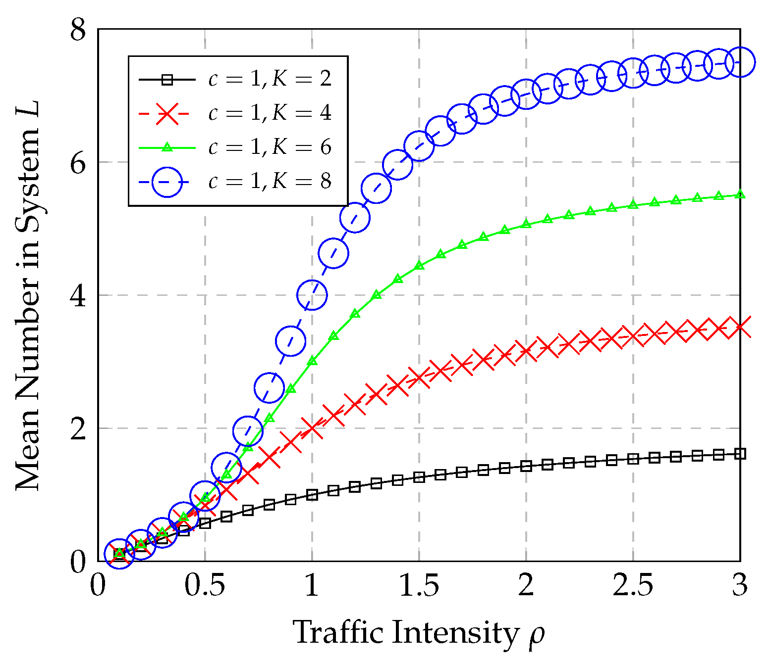
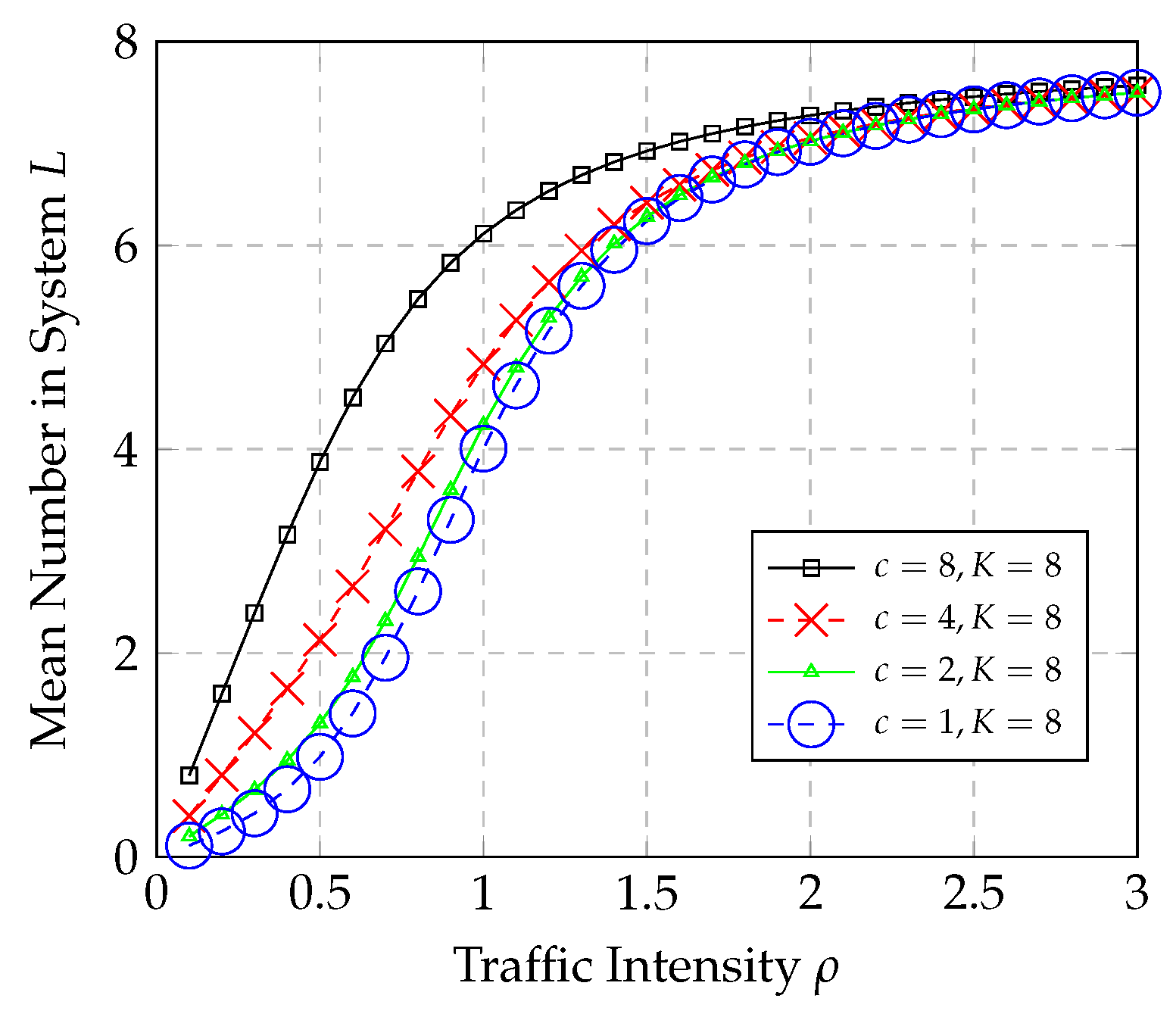
The graphs in Figure 2 show the results of the mean number of items in the M/M/1/K system for varying traffic intensity $\rho$ (with $1\le \lambda \le 24$ and $\mu =8$), and for a system capacity of $K=\left\{2,4,6,8\right\}$. Furthermore, the graphs in Figure 3 show the results of the mean number in the system for an M/M/c/K system for varying $\rho$ (with $\mu =8$) and with varying number of servers $c=\left\{1,2,4,8\right\}$. For this M/M/c/K system, the graph of L for a large $K+c$ shows the same pattern as that for the M/M/1/K for a large K.

From Equation (3), it is clear that $L=0$, when $\rho =0$, which should be intuitive. Also, for a fixed K, it can be shown that the limit

$$\underset{\rho \to \infty }{lim}L=K.$$

(5)

Secondly,

$${\displaystyle \frac{dL}{d\rho }}\ge 0,$$

(6)

and we observe that

$${\displaystyle \frac{d^{2}L}{d{\rho }^2}}\le 0,\mathrm{when}\rho >1.$$

(7)

Generally, L seems to be a concave function of $\rho$ when $\rho >1$ for specific values of K.

Based on these, one can potentially approximate L by an equation of the form

$$L\approx V_K{\displaystyle \frac{\rho }{K_K+\rho }}.$$

(8)

By plotting the values of L versus $\rho$ for a fixed K, we find that the plot satisfies Equation (5) for a large K, as shown later.

5. Machine Learning Tools for Studying L

In this work, we propose analyzing L as a regression problem and present the case for adopting the M-M model as a machine learning algorithm to forecast L in a queueing system for a given parameter such as $\rho$ (or $\lambda$ for a fixed $\mu$). There are various and other regression models that may also be adopted for the supervised learning model [37]. However, our aim is not to assess and find the best-fit model, but rather to demonstrate the effectiveness of applying machine learning for analyzing queueing systems as an alternative to mathematical analysis. For simplicity, we opted to utilize the M-M model and show how it may be a reasonable fit. We intend to explore other and better-fit models in our future work. Figure 4 shows an overview of the solution we are proposing for forecasting a queueing system’s performance, specifically in terms of L. We stress again that this solution is not intended as a replacement to the mathematical models and the exceptional efforts spent in deriving the analytical solutions to queueing models. It is instead offered as an alternative method, especially for large and complex systems with solutions that are mathematically intractable. This machine learning approach is easier and faster to implement, though it is an approximation.

5.1. Observations Regarding Behavior of L

One of the key observations to note from the results shown in Figure 2 and Figure 3 is that the plots of L increase in a common pattern with increasing K. The graphs in Figure 2 show the results of the mean number of items in the M/M/1/K system for varying traffic intensity $\rho$ (with $1\le \lambda \le 24$ and $\mu =8$), and for a system capacity of $K=\left\{2,4,6,8\right\}$. Based on the results shown in Figure 2 and Figure 3, as K increases, the shape of the curve tends more to one that looks like the M-M curve, specifically after $\rho >1$. Thus, for a large K, which is the region we are focusing on, one can conjecture that the curve is of that pattern. This experiment suggests that one can estimate the L for M/M/c/K systems with large K using the M-M equation in supervised machine learning. The following are a set of other important observations regarding the fitting of the M/M/c/K system behavior to the M-M model:

• $V_{max}\approx K$ in all cases;
• Letting the $n^{th}$ order estimate of $V_{max}$ be written as $V_{max}^n$, we notice that $V_{max}^1\ge V_{max}^2.$

These observations provide some strong confidence in pursuing further the idea of adopting the M-M model in the ML tool for estimating the performance of a queueing system.

Machine learning tools are of several types and one of the most popular and easy to use is supervised learning. We selected the non-linear regression tools of machine learning for this class of problems because they appeared an appropriate choice. There is a very good similarity in terms of shape between the graph of L versus $\rho$ and the graph of kinetics in biochemistry. Thus, we capitalize on this similarity in developing our ML model.

5.2. Relation of L to Michaelis–Menten Equation

After reviewing the values of L versus $\rho$ for any K, we notice that the results have a similar shape and behavior to the M-M model. By virtue of the fact that the plot of v versus $\left[S\right]$ in the M-M model has the same pattern as the plot of L versus $\rho$ for a fixed K in the M/M/c/K model, it becomes clear the non-linear regression models developed for the M-M model would be a good supervised machine learning model to use for estimating the mean queue length for the M/M/c/K model, where the $V_{max}$ and the $K_m$ in the M-M model would be equivalent parameters that capture the K and $\rho$ for the M/M/c/K, and $\left[S\right]$ in the M-M would specifically be equivalent to the $\rho$ in the M/M/c/K model.

We conjecture that in Equation (8) for L, $\rho$ is the traffic intensity, and both $V_k$ and $K_k$ depend on the value of K, and may also depend on $\rho$. Equation (8) is a simplified model and can be refined further after detailed studies. One expected behavior of the parameter $V_K$ is that for any M/M/c/K, $V_K$ should tend to K with increasing $\rho$; hence, ${\displaystyle \frac{\rho }{K_K+\rho }}$ should tend to one for large $\rho$.

5.3. Using M-M Fitting Method for L Equation

Touilas and Kitsos (2016) [38] showed non-linear regression methods for the M-M equation. However, other methods are available in the literature for the same purpose, such as by Atkins and Nimmo (1975) [39]. Software tools, such as MATLAB (version 2022a), can also be used for evaluating the best-fit M-M model. We sought a simple approach that is practical to use and adopt in this work.

6. M-M Fitting for Mean Number L of M/M/c/K Systems

In this section, we present the results of the parameters $V_{max}$ and $K_{max}$ of the M-M model from Equation (1) that best model the mean number L in the M/M/c/K system and for the numerical examples shown in the previous section. The built-in function nlinfit in MATLAB was used to determine the values of the parameters for the best-fit M-M model.

Table 1. Best-fit parameters of M-M model for M/M/1/K systems.

	${\mathit{V}}_{\mathit{max}}$	${\mathit{K}}_{\mathit{max}}$	${\mathit{R}}^2$
M/M/1/2	2.28	1.28	99.4%
M/M/1/4	5.17	1.52	96.5%
M/M/1/6	8.13	1.58	93.5%
M/M/1/8	11.1	1.59	90.9%

shows the values of the coefficients $V_{max}$ and $K_{max}$ that were computed for the M-M model that best fit the results that were evaluated for the mean number L in the M/M/1/K systems shown in Figure 2. For determining the best-fit model, we included additional results from the analytical solutions for up to $\rho =5$ to determine the coefficients of the M-M model. The table also includes the value for the coefficient of determination $R^2$, which provides a measure for the goodness-of-fit.

The graphs in Figure 5 and Figure 6 illustrate how well the best-fit M-M model compares with analytical results for the mean number in the M/M/1/4 and M/M/1/8 systems, respectively.

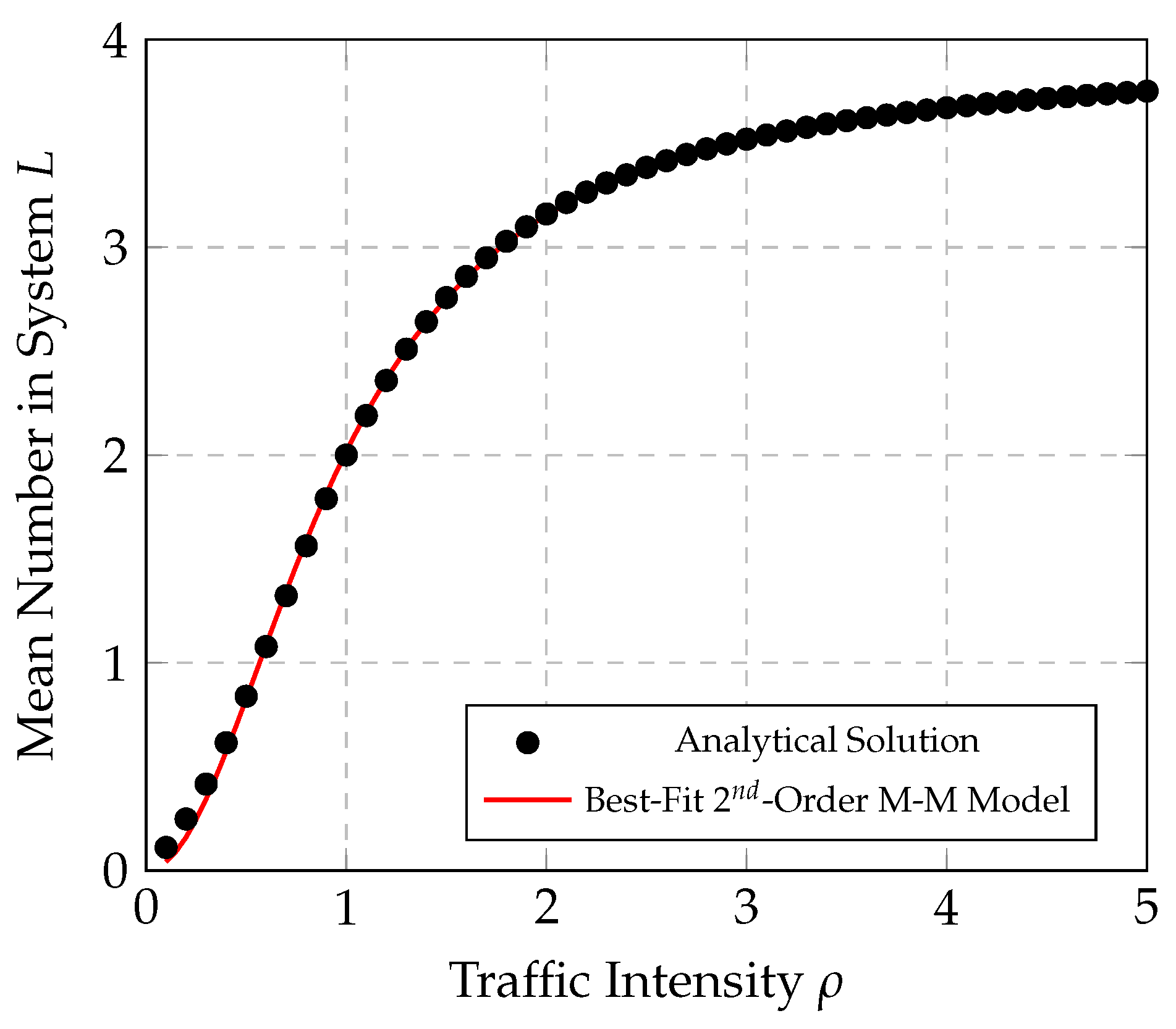
These results demonstrate how well the M-M model can characterize the behavior for the mean number in M/M/1/K systems, when $\rho >1$. The goodness-of-fit $R^2$ is high for these examples, but decreases with increasing buffer capacity K. The results could be improved if a second-order M-M model was used instead for the fitting process, with the form of the second-order model shown as follows:

$$v=V_{max}{\displaystyle \frac{{\left[S\right]}^2}{K_{max}+{\left[S\right]}^2}}.$$

(9)

Table 2. Best-fit parameters of second-order M-M model for M/M/1/K systems.

	${\mathit{V}}_{\mathit{max}}$	${\mathit{K}}_{\mathit{max}}$	${\mathit{R}}^2$
M/M/1/2	1.76	0.74	98.2%
M/M/1/4	3.89	0.93	99.9%
M/M/1/6	6.09	0.98	99.4%
M/M/1/8	8.31	0.99	98.2%

shows the values of the coefficients for the second-order M-M model that provided the best fit for the mean number L in the same M/M/1/K systems shown in Figure 2. These results show an overall higher goodness-of-fit $R^2$. These improvements are further demonstrated by the results shown in Figure 7 and Figure 8 that compare the best-fit second-order M-M model with the analytical results for the mean number in the M/M/1/4 and M/M/1/8 systems, respectively. Note how these results show that the second-order M-M model yielded a better fit compared to the ones shown in Figure 5 and Figure 6.

After establishing that the machine learning tool works reasonably well for the M/M/1/K system, the analysis was repeated to determine the best fit model for the mean number in an M/M/c/K system and for the numerical examples shown in Figure 3. For determining the best-fit model, we included additional results from the analytical solutions for up to $\rho =5$ to determine the coefficients of the M-M model.

Table 3. Best-fit parameters of first-order M-M model for M/M/c/8 systems.

	${\mathit{V}}_{\mathit{max}}$	${\mathit{K}}_{\mathit{max}}$	${\mathit{R}}^2$
M/M/2/8	10.8	1.43	92.2%
M/M/4/8	10.0	1.08	94.8%
M/M/8/8	8.92	0.54	96.8%

and

Table 4. Best-fit parameters of second-order M-M model for M/M/c/8 systems.

	${\mathit{V}}_{\mathit{max}}$	${\mathit{K}}_{\mathit{max}}$	${\mathit{R}}^2$
M/M/2/8	8.23	0.89	98.9%
M/M/4/8	8.03	0.64	99.6%
M/M/8/8	7.77	0.25	99.4%

include the coefficients of the best-fit M-M model and the second-order M-M model, respectively. Furthermore, Figure 9 and Figure 10 show the difference in the best-fit first-order and second-order M-M model for the mean number in M/M/2/8 and M/M/4/8 systems, respectively. These results also highlight how well the M-M model fits analytical results for evaluating the mean number in M/M/c/K systems.

7. Extension of ML Results to PH/PH/1/K and GI/G/1/K Models

To further assess our proposed solution, we ran several experiments for other related single-server queueing systems, including the PH/PH/1/K system. The graphs in Figure 11 show the results of the mean queue lengths for a PH/PH/1/K system that is modeled as a discrete-time Markov chain. The arrival process is modeled as a phase-type distribution with parameters $\left(\alpha ,T\right)$ and the service process is modeled as a phase-type distribution with parameters $\left(\beta ,S\right)$. The following phase type distributions were considered in this numerical example.

$$\alpha =\left[0.2,0.8\right],T=\left[\begin{array}{cc}0.3\tau & 0.4\\ 0.2\tau & 0.5\end{array}\right],\beta =\left[0.7,0.3\right],S=\left[\begin{array}{cc}0.5& 0.3\\ 0.3& 0.55\end{array}\right].$$

Using these values, the mean service time in this example is $5.67$, whereas the mean arrival time varies between $1.96$ and $20.5$ as $\tau$ is varied between 0 and 2. Hence, this example considers the cases for the arrival rate $0.05\le \lambda \le 0.51$ with $2\ge \tau \ge 0$, and with a constant service rate of $\mu =0.18$, along with $\rho =\lambda /\mu$.

We observe that the mean number in the system has the same pattern when L is plotted against $\rho$; see Figure 11. Hence, the ML tool we developed is robust and can be used to study PH/PH/1/K systems and also GI/G/1/K systems in discrete time. The limitations of our model are that it is for the mean number in the system and cannot be used for studying the probability distributions of the number in the system.

A best-fit M-M model was also evaluated for the PH/PH/1/K numerical examples shown in Figure 11.

Table 5. Best-fit parameters of first-order M-M model for PH/PH/1/K systems.

	${\mathit{V}}_{\mathit{max}}$	${\mathit{K}}_{\mathit{max}}$	${\mathit{R}}^2$
PH/PH/1/4	7.83	2.79	96.5%
PH/PH/1/6	13.4	3.30	93.3%
PH/PH/1/8	19.0	3.54	90.5%
PH/PH/1/10	24.7	3.67	88.2%

and

Table 6. Best-fit parameters of second-order M-M model for PH/PH/1/K systems.

	${\mathit{V}}_{\mathit{max}}$	${\mathit{K}}_{\mathit{max}}$	${\mathit{R}}^2$
PH/PH/1/4	4.24	1.02	99.9%
PH/PH/1/6	6.79	1.17	98.9%
PH/PH/1/8	9.37	1.23	97.3%
PH/PH/1/10	11.9	1.27	95.8%

include the coefficients of the best-fit M-M model and the second-order M-M model, respectively, and for different PH/PH/1/K systems. Furthermore, Figure 12 and Figure 13 show the differences in the best-fit first-order and second-order M-M model for the mean number in PH/PH/1/4 and PH/PH/1/10 systems, respectively. These results also demonstrate that the mean number in PH/PH/1/K systems could also be described numerically by an M-M model.

Conjecture About Family of GI/G/c/K System

From the basic knowledge we have considered of how queueing systems behave, it is clear that the maximum mean number in the system is $Kc$ for the GI/G/c/K system. Secondly, it is known from the literature that GI/G/c/K systems can be approximated by PH/PH/c/K, especially discrete-time cases. Hence, one can conjecture that the same ML model can be used for studying such systems, since the mean number in such a system increases as $\rho$ increases for a fixed set of c and K. This will be pursued at a later next stage of our research; meanwhile, we focus on the M/M/c/K system, which will guide us into the GI/G/c/K machine learning model at a later stage of our research.

8. Extension of ML Tool to Tandem Queues

Given that the idea looks reasonable for the single-node queue, we extend the result to tandem queues with finite buffers. Most communication networks consist of several tandem queues all with finite buffers. Consider two finite queues in tandem where the first queue is an M/M/1/K₁ system and the output from that queue is fed into a ./M/1/K₂ system.

In this system, we assume that a job departing from the first queue after service completion moving into the second queue that is full will not be dropped from the system and will instead wait until one departs from the second queue. During that time, no jobs are being served from the first queue. The analysis of such a system was conducted for evaluating the mean number in the first and second queue, as well as overall, under varying arrival rates. In our numerical analysis, we assume the service rates in the first and second queue are ${\mu }_1=6$ and ${\mu }_2=5$, respectively.

Figure 14 shows the behavior of the mean number in the tandem queue system with varying traffic intensity, which is defined as $\rho =\lambda /\breve{\mu }$, where $\breve{\mu }=min\left\{{\mu }_1,{\mu }_2\right\}$. Note that the number in the tandem queue system corresponds to the total number of items waiting in both queues, along with the items undergoing service in both servers. The results are shown for varying arrival rates $1\le \lambda \le 25$ ( ${\mu }_1=6$ and ${\mu }_2=5$) and for different capacities $K_1$ in the first queue with a fixed capacity of $K_2=5$ in the second queue. Figure 15 shows a similar set of results but instead for a fixed capacity of $K_1=5$ in the first queue and for different capacities $K_2$ in the second queue. Once again, we notice that the plots of the mean number in the tandem queue system follow the same pattern as that of the single node queues. Hence, it is a candidate for the application of supervised machine learning using non-linear regression tools based on the M-M model.

M-M Fitting for Mean Number L in System of Tandem Queues

We adopt the same process used in Section 6 for determining the coefficients of the best-fit M-M model and for the case of the tandem queue system example. For evaluating the results, we will focus on the case of finding the best-fit M-M model for the overall mean number in the system with two tandem queues and buffer capacities $K_1=\left\{4,6,8\right\}$ and $K_2=5$, i.e., the case that corresponds to the results shown in Figure 14.

Table 7. Best-fit parameters of first-order M-M model for tandem queue systems.

	${\mathit{V}}_{\mathit{max}}$	${\mathit{K}}_{\mathit{max}}$	${\mathit{R}}^2$
M/M/1/4 → ./M/1/5	9.61	1.18	92.2%
M/M/1/6 → ./M/1/5	12.3	1.16	89.3%
M/M/1/8 → ./M/1/5	15.0	1.17	87.1%

and

Table 8. Best-fit parameters of second-order M-M model for tandem queue systems.

	${\mathit{V}}_{\mathit{max}}$	${\mathit{K}}_{\mathit{max}}$	${\mathit{R}}^2$
M/M/1/4 → ./M/1/5	7.61	0.71	99.2%
M/M/1/6 → ./M/1/5	9.79	0.70	97.9%
M/M/1/8 → ./M/1/5	12.0	0.71	96.7%

show the coefficients of the best-fit M-M model and the second-order M-M model, respectively, and for the three different tandem queue systems. Furthermore, Figure 16 and Figure 17 show the difference in the best-fit first-order and second-order M-M model for the mean number in the tandem queue systems with $K_1=4$ and $K_1=8$, respectively. These results provide some confidence in the ability of the M-M model in characterizing the behavior of the overall mean number in a system of two tandem queues.

The results so far has provided reasonable confidence in the ability of the M-M model to be used for characterizing the mean number in the system for single-node and tandem queues. Thus, we can proceed with applying the model to a complex system.

9. Network of Queues with Feedback

The application of the proposed ML tool was further examined on a complex system comprising a network of queues with feedback. Such systems are generally quite challenging to model analytically, especially in cases that involve a large number of queues. We recall that one of our goals is to develop a tool that is simple and scalable for analyzing large and complex queueing systems. To demonstrate the performance of the proposed ML tool, we considered the example shown in Figure 18.

For the analysis in this example, we assumed the service time in each of the four single-server queues to be exponentially distributed with the fixed set of rates ${\mu }_1=9$, ${\mu }_2=8$, ${\mu }_3=7$, and ${\mu }_4=6$, with the queue capacities $K_1=K_2=K_3=10$ and $K_4=8$. Note that queue capacities $K_i,i=1,2,3,4,$ include the waiting space capacity plus the one in service. The routing probabilities $p_{ij}$ in Figure 18 were assigned as follows: $p_{21}=0.2$, $p_{23}=0.8$, $p_{31}=0.5$, $p_{34}=0.5$, $p_{40}=0.75$, and $p_{44}=0.25$. The external inter-arrival times into the first two queues were also assumed to be exponentially distributed and the arrival rate into the second queue was assigned as ${\lambda }_2=1$. Unlike the case in Section 8, we assumed that entities arriving into a full queue are dropped and discarded from the system, regardless of whether these arrivals are from external entities or are fed back in from other queues. This assumption was necessary since the contrary could lead to the case where the queues are all full and then the system is in a locked state that prevents them from routing packets to other queues that are in the same locked state.

Deriving the mathematical model for this complex system is usually laborious, especially when it includes a larger number of queues. Even if it is successfully carried out, the computational task is a challenge. A simulation of the system was instead developed for evaluating the overall mean number in the system. The analysis was conducted for a varying external arrival rate ${\lambda }_1$ (between 1 and 20), with all other system parameters remaining unchanged. The graph in Figure 19 shows how the mean number in the network varies with the external arrival rate ${\lambda }_1$. The same figure also includes the best-fit M-M model for the overall mean number in the system for both the first-order and second-order models. Due to the complexity in evaluating $\rho$ for this system, we opted to use ${\lambda }_1$ instead of $\rho$ for determining the best-fit M-M model since $\rho$ is a function in terms of ${\lambda }_1$. The use of ${\lambda }_1$ in place of $\rho$ also allows us to examine the robustness of the proposed technique. The coefficients for the best-fit M-M model are shown in

Table 9. Best-fit parameters of first-order and second-order M-M model for network of queues with feedback system and with varying ${\lambda }_1$.

	${\mathit{V}}_{\mathit{max}}$	${\mathit{K}}_{\mathit{max}}$	${\mathit{R}}^2$
First-Order Model	26.1	2.69	96.1%
Second-Order Model	22.2	5.38	99.6%

.

The analysis was repeated for the same system but for instead the case where the external arrival rate ${\lambda }_2$ is varied between 1 and 20, with ${\lambda }_1=2$ being fixed in the system and all other parameters remaining the same as those assigned in the previous analysis. The graphs in Figure 20 show the overall mean number in the system for this analysis along with its best-fit M-M models, whose coefficients are given in

Table 10. Best-fit parameters of first-order and second-order M-M model for network of queues with feedback system and with varying ${\lambda }_2$.

	${\mathit{V}}_{\mathit{max}}$	${\mathit{K}}_{\mathit{max}}$	${\mathit{R}}^2$
First-Order Model	18.8	0.84	99.2%
Second-Order Model	17.5	1.01	94.6%

. In general, these results highlight the suitability and potential for applying the M-M model in learning algorithms for analyzing the overall mean number in a complex system composed of a network of queues, such as the one examined in this section of the analyses. The one interesting find from these results is the $R^2$ measure in Table 10, which suggests that a first-order M-M model would provide a better fit for the particular case of the complex system than the second-order model, which is the opposite of what had been discovered in the analyses of the less complex systems covered in the previous sections. This finding merits further investigation in our future work.

10. The Practical Advantage of This Machine Learning Tool

For most real-life systems, even if we know that a system in question is a finite buffer system with multiple servers, we usually do not know the arrival or service processes. These processes have to be determined first. Fitting a specific probability distribution to either the arrival process or the service process is an arduous task. For example, consider the inter-arrival times: are they exponential, phase type (PH), or associated with other types of distributions? If we think they are PH, we then have to find the best statistically fitting PH. This opens up a new set of problems. What structure of the PH distribution can we assume and what is the dimension of the PH? These are few of the questions that need to be asked and a considerable amount of research has been carried out on this subject—the available results are good but still require considerable amount of effort to implement, thereby steering some applied researchers away from this topic.

After all these have been resolved, one then has to analyze a Markov chain with a transition probability matrix of at least size $Knm\times Knm$ for the PH/PH/1/K system, with PH arrival and service matrices of dimensions $n\times n$ and $m\times m$, respectively, just for a simple single-server queueing case! For most real-life systems, the size of K is usually large. In the end, simple assumptions about the arrival processes are made for expediency. This issue is also the same with the service process. With this machine learning tool, all we need are the average arrival and service rates $(\lambda ,\mathrm{and}\mu )$ and the observed sets of queue lengths $\left(L\right)$. We can then apply the supervised learning ML tool, which will determine the appropriate M-M parameters that best match the observed data.

Given a set of n observations of ${\lambda }_i,{\mu }_i,$ and $L_i,i=1,2,\cdots ,n$, we then apply the M-M regression model to find the best parameters $V_{max}$ and $K_{max}$ that best fit the data, so we can have

$$L=V_{max}{\displaystyle \frac{\rho }{K_{max}+\rho }}.$$

(10)

11. Conclusions

In this paper, we have demonstrated that single- and tandem-node finite buffer queues can be analyzed using machine learning, and showed that the idea can be extended to tandem complex finite buffer queues with feedback. When an analyst is tasked with studying such queues, they must first gather data on the arrival process, service process, and queue lengths. This data can then be utilized in the machine learning model to estimate the mean number of items in the queueing system. The machine learning model provides the necessary parameters of the M-M function, which can then be used to analyze the system. It is important to note that the information on buffer sizes is not always necessary, especially in some communication networks, where such parameters may not be clearly defined. Additionally, analysts do not need to specify the probability distributions associated with the arrival and service processes, as the focus is solely on the mean number of items in the system. We have demonstrated that this concept can be extended to tandem queues with and without feedback. The coefficient of determination $R^2$ for all the examples presented are all higher than $90\%$, with some as high as $99.6\%$. This is very encouraging and suggests that this approach be pursued further.

Our proposed solution is based on non-linear regression of two parameters and utilizes standard techniques for evaluating the best-fit parameters for the Michaelis–Menten model. In general, such computations are significantly less complex and require very short computational run times when compared with simulations. For example, the simulation of the system in Figure 18 had an average runtime of 167 s for each variation in the traffic intensity, whereas the parameter fitting computations were completed in under 1 s. Furthermore, our proposed solution is independent of the system’s complexity and avoids the need to develop complex simulations. In addition, once the best-fit parameters are evaluated using the data from the system, the result can be used to immediately predict the mean number in the system L for any traffic intensity $\rho$ (or arrival rate $\lambda$). Meanwhile, a simulation would typically require more computational time and resources, and would need to be repeated for different values of $\rho$ (or $\lambda$). Thus, the computation time and computational complexity of the proposed solution are negligible when compared with the method of evaluating the system’s performance using simulations.

In our future work, we intend to explore the application of our proposed method on other and more complex network of queues, along with systems that exhibit complex inter-arrival and service time behaviors. We further intend to examine the performance of the proposed solution on non-Markovian queueing systems and for cases with dynamic traffic intensities. If the prospect of studying these types of queues using supervised learning based on the Michaelis–Menten method can be validated, then we may be able to develop effective machine learning methods for studying queueing networks with finite buffers, and for possibly considering other regression models.