A New Method for the Exact Controllability of Linear Parabolic Equations

Abstract

This work solves the exact controllability to zero in the final time for a linear parabolic problem when the control only acts in a part of the spatial domain. Specifically, it is proved, by compactness arguments, the existence of a partially distributed control. The lack of regularity in the problem prevents the use of standard techniques in this field, that is, Carleman’s inequalities. Controlling a parabolic equation when the diffusion is discontinuous and only acts in a part of the domain is interesting, for example, as in the spreading of a brain tumor. The proof is based on a new maximum principle in the final time; in a linear parabolic equation, with a right-hand side that changes sign in a certain way, and an initial datum of a constant sign, the solution at the final time has the same sign as the initial datum. As a consequence of the exact control result, we prove a unique continuation theorem when the data are not regular.

1. Introduction

The goal of this work is to solve an exact control problem to zero, with partially distributed control, in a linear parabolic equation. The particularity of this equation is that the diffusion coefficients are functions whose regularity conditions are not required and the smoothness of $\partial \Omega$ is not assumed either.

Specifically, we study the exact control to zero, with partially distributed control, of the problem

$$\left\{\begin{array}{c}{y}_t-\nabla ·(A\nabla y)=u{1}_{\omega }\mathrm{in}\Omega \times (0,T)\hfill \\ {y|}_{\Sigma }=0\hfill \\ y(0)=y_0\mathrm{in}\Omega ,\hfill \end{array}\right.$$

(1)

where $\Omega$ is a bounded domain in ${\mathbf{R}}^N$ and its boundary, $\partial \Omega$, is piecewise smooth, i.e., $\partial \Omega \in C^{0,1}$. Note that $y(x,t)$ is the solution of the problem depending on space and time and $1_{\omega }$ is the indicator function, i.e., a spatial function that values 1 if $x\in \omega$ and 0 if $x\in \Omega \backslash \omega .$ We only need to ask the necessary regularity to define the trace, to be able to integrate by parts, to have the existence and uniqueness of the solution of the boundary–initial value linear parabolic problem, and it is a verified Rellich–Kondrachoff theorem (see Remark 16.1 in [1]). As far as we know, this is the first paper to prove the controllability of a parabolic equation for arbitrary Lipschitz domains.

The set where the control acts is $\omega$, and it is an open set contained in $\Omega$. We write $\Sigma$ to mean $\partial \Omega \times (0,T)$, $y_0$ is a function in $L^2(\Omega )$, and A is a matrix whose coefficients are functions in $L^{\infty }(\Omega \times (0,T))$ satisfying the following condition:

$$\alpha \sum _{i=1}^N{\xi }_i^2\le \sum _{i,j=1}^N{A}_{ij}(x,t){\xi }_i{\xi }_j\le \mu \sum _{i=1}^N{\xi }_i^2,\alpha ,\mu >0.$$

(2)

The question we answer in the affirmative is the following.

Is it possible to find $u\in L^2(\Omega \times (0,T))$ such that the solution y of (1) verifies $y(T)=0$ in $\Omega$?

It is well known that if it is possible to control to zero the solution of a linear problem, then we can drive the solution to any trajectory.

The question of controlling acting on a part of the domain has practical interest.

Studying the control of problems like (1) can be interesting in modeling the spreading of a brain tumor. In [2], the authors solve numerically a linear parabolic problem where the diffusion coefficients are not continuous: the spreading of the tumor cells in white matter of the brain is faster than in the grey one. To be able to control a problem with non-smooth coefficients may be of great interest.

Although the procedure consists of obtaining a control for non-negative initial data, this does not represent a restriction. Once control is achieved, it is enough to consider the positive and negative parts of the initial data and the difference in both controls provides a control for any initial data. In this work, we do not analyze the control problem, preserving the positivity of the state. For this type of problem, see the references [3,4].

The null controllability is known when the diffusion operator is the Laplacian or when the diffusion coefficients are regular. In [5], the authors provide an overview of the null controllability and the exact controllability to the trajectories of some relevant linear and nonlinear parabolic systems. They consider the classical heat equation with Dirichlet conditions and distributed controls. In this framework, the global Carleman estimates are known, and they allow to obtain an observability inequality in order to conclude that the null controllability of the heat equation with Dirichlet boundary conditions and partially distributed controls has a solution. The use of Carleman estimates limits the controllability to problems with diffusion coefficients in $C^1(\Omega )$ and $\partial \Omega$ also regular.

In [6], the authors perform a study of the null controllability of the heat equation for a $C^{\infty }$ variety of the Riemann. The estimations of the elliptic operator ${\partial }^2/\partial t^2+\Delta$, via Carleman inequalities, require the smoothness of the coefficients.

When the parabolic equation is semilinear, the work of Emanuilov [7] studies the exact controllability if the control is distributed over an arbitrary subdomain $\omega$ of $\Omega$ and if the control is distributed over a subdomain of $\partial \Omega$. The nonlinearity is globally Lipschitz. The control problem is solved controlling the linear problem and building a continuous map that has a fixed point. The controllability of the linear parabolic equation is based on an a priori estimate of the Carleman type with a certain singularity. The smoothness of $\partial \Omega$ is $C^2$.

Recently, in the multidimensional case with non-smooth data, the controllability is obtained for some particular problems. In [8], the authors prove Carleman estimates for operators with discontinuities of the coefficients in one direction. The derivation of the Carleman inequality requires that $\Omega$ is a band domain, $\Omega ={\Omega }^{\prime }\times (-H,H)$, and $\partial {\Omega }^{\prime }$ is $C^1$. In [9], Carleman inequalities are obtained for a more general operator, although the case where the diffusion coefficients are totally anisotropic is left open, and it is required that $\partial {\Omega }^{\prime }$ is $C^2$. The assumption of regularity $C^2$ is also imposed in [10] besides some geometrical constraints on $\Omega$.

In the one-dimensional case, the null controllability is proved in [11] when the diffusion coefficient is bounded and it does not depend on the variable t. The authors obtain a distributed control, in one spatial dimension, following the procedure of the spectral decomposition. The null controllability for the heat equation via an observability inequality is obtained in [12]. The authors find out non-smooth weight functions for a Carleman inequality, but the hypothesis of one dimension is essential. In [13], when the control is a boundary and the coefficients are not regular but independent on time, the linear heat equation in one dimension is controlled by the control of the one-dimensional wave equation.

For transmission problems with regular coefficients and jump in the interface, the exact control to trajectories is studied in [14]. The idea is to use approximate controllability to zero. Some constraints on the domains and on the regularity of the coefficients are imposed.

The results of this work are novel, as far as we know. We do not need constraints of smoothness on the domain, nor on the coefficients, which can depend on time, there is no restriction on the spatial dimension of $\Omega$, and we obtain an explicit formula of the control.

The method consists of starting from a non-negative function u in $\Omega \times (0,T)$ and we obtain a non-negative function $v^{*}$ that verifies that

$$\parallel y(T)\parallel {\Psi }_{v^{*}}(T)-\parallel {\Psi }_{v^{*}}(T)\parallel y(T)$$

is identically equal to zero in $\Omega$, being that y is the solution of (1) with $y_0\ge 0$, and ${\Psi }_{v^{*}}$ is the solution of (1) with the right-hand side $v^{*}{1}_{\omega }$ and the same initial data $y_0$ ($\parallel ·\parallel$ denote the norm in $L^2(\Omega )$).

We prove the following result of controllability:

Theorem 1.

Let be $u\in L^2(\omega \times (0,T))$, $u\ge c>0$ in $\omega \times (0,T)$ and zero outside of ω, $y_0\in L^2(\Omega )$, $y_0\ge 0$. Then, there exists $v^{*}\in L^2(\omega \times (0,T))$, $0\le v^{*}\le u$, $\parallel {\Psi }_{v^{*}}(T)\parallel < \parallel y(T)\parallel$ such that

$${\displaystyle \widehat{u}=\frac{\parallel y(T)\parallel v^{*}-\parallel {\Psi }_{v^{*}}(T)\parallel u}{\parallel y(T)\parallel -\parallel {\Psi }_{v^{*}}(T)\parallel }}$$

is a control in ω for the initial data $y_0$.

When the initial data are any function $y_0\in L^2(\Omega )$, we apply this theorem with $y_0^{+}$ and $y_0^{-}$.

The control result also provides a fixed-point equation for the solution in $t=T$ of a problem such as (1) when the second member and initial data are non-negative. Specifically, we have that if y is the solution of (1) with u and $y_0$ non-negative, then there exists a non-negative function $v^{*}$ such that

$${\displaystyle \frac{y(T)}{\parallel y(T)\parallel }=\frac{{\Psi }_{v^{*}}(T)}{\parallel {\Psi }_{v^{*}}(T)\parallel }.}$$

A uniqueness result can be deduced by the control result.

Theorem 2.

If φ verifies

$${\phi }_t-\nabla ·(A(x,t)\nabla \phi )=0\mathrm{in}\Omega \times (0,T),$$

$${\phi |}_{\Sigma }=0$$

and

$$\phi =0\mathrm{in}\omega \times (0,T),$$

then it is necessary that

$$\phi \equiv 0\mathrm{in}\Omega \times (0,T).$$

In [15], a unique continuation result is proved but it uses the smoothness of the coefficients.

The work is divided as follows: In Section 2, we prove a maximum principle at the final time T. This result is the key to prove the exact control in Section 3. The main result in this section is Theorem 5. The reasoning is the following:

• We suppose that the initial data of the solution that we want to drive to zero, $y_0$, are non-negative.
• Given a non-negative function u in $\Omega \times (0,T)$, we prove the existence of an exact control in the whole spatial domain $\Omega$. This is performed in Theorem 4. The control $\widehat{u}$ is given by u and a function $v^{*}$.
• Now, thanks to Theorem 4, we can prove the existence of a partially distributed control.
• Once we have proven the existence of a partially distributed exact control to zero, when $y_0\ge 0$, it is easy to obtain a control for any $y_0$ if we consider $y_0$ as the sum of its positive and negative parts. Then, we apply Theorem 5 to each ones, and the final control is the sum of the two controls.

In Section 4, a unique continuation result is deduced. Finally, we show some numerical results for a parabolic problem with non-smooth coefficients and conclusions.

We will write $(·,·)$ to indicate the scalar product in $L^2(\Omega )$ or the duality product $H^{-1}(\Omega )\times H_0^1(\Omega )$, $\parallel ·\parallel$ the norm in $L^2(\Omega )$, and $<·,·>$ the scalar product in $L^2(\Omega \times (0,T))$ or the duality product $L^2(0,T;H^{-1}(\Omega ))\times L^2(0,T;H_0^1(\Omega ))$.

We denote $W(0,T)$ as the space

$$W(0,T)=\{w\in L^2(0,T;H_0^1(\Omega )):{\displaystyle \frac{dw}{dt}}\in L^2(0,T;H^{-1}(\Omega ))\}.$$

To simplify, we write the Laplacian operator $-\Delta$ in the place of $-\nabla ·(A(x,t)\nabla )$. The key points of the proofs are the linearity of the differential equation and the maximum principle. This is true when the diffusion coefficients are not regular. In [16], page 188, the maximum principle is stated if the coefficients $A_{ij}$ verify the conditions of coercivity and boundness given by (2).

Definition 1.

For any function $w\in L^2(\omega \times (0,T))$, we define ${\Psi }_w$ as the solution of the problem

$$\left\{\begin{array}{ccc}{({\Psi }_w)}_t-\Delta {\Psi }_w=w\hfill & \mathrm{in}& \hfill \Omega \times (0,T)\\ {\Psi }_w=0\hfill & \mathrm{on}& \hfill \partial \Omega \times (0,T)\\ {\Psi }_w(0)=y_0\hfill & \mathrm{in}& \hfill \Omega .\end{array}\right.$$

(3)

For the case of $w=u$ or $w=u{1}_{\omega }$ the solution of the problem will be denoted by y:

$$\left\{\begin{array}{ccc}{y}_t-\Delta y=u\hfill & \mathrm{in}& \hfill \Omega \times (0,T)\\ y=0\hfill & \mathrm{on}& \hfill \partial \Omega \times (0,T)\\ y(0)=y_0\hfill & \mathrm{in}& \hfill \Omega \end{array}\right.$$

(4)

or

$$\left\{\begin{array}{ccc}{y}_t-\Delta y=u{1}_{\omega }\hfill & \mathrm{in}& \hfill \Omega \times (0,T)\\ y=0\hfill & \mathrm{on}& \hfill \partial \Omega \times (0,T)\\ y(0)=y_0\hfill & \mathrm{in}& \hfill \Omega .\end{array}\right.$$

(5)

2. A Maximum Principle at the Final Time

We begin with a result which is the key of the work. It consists of proving that if the right-hand side of a parabolic linear problem changes of sign, under some hypothesis, and the initial data has a constant sign, then the solution at the final time has the same sign than the initial data. It is a maximum principle only at the final time.

Theorem 3.

Let be $\beta \in C^1([0,T])$ verifying

$$\begin{array}{c}\beta >0\hfill \\ {max}_{[0,T]}\beta =\beta (T),\hfill \end{array}$$

(6)

and let be $w\in W(0,T)$ such that

$$\left\{\begin{array}{c}{w}_t-\Delta w\ge 0\hfill \\ {w|}_{\Sigma }=0\hfill \\ w(0)\ge 0.\hfill \end{array}\right.$$

(7)

Then, the solution z of the problem

$$\left\{\begin{array}{c}{z}_t-\Delta z=-{\beta }^{\prime }w\hfill \\ {z|}_{\Sigma }=0\hfill \\ z(0)=z_0\le 0.\hfill \end{array}\right.$$

(8)

verifies

$$z(T)\le 0.$$

Remark 1.

If β is increasing, the statement of Theorem 3 follows from the classical comparison theorem since in this case $-{\beta }^{\prime }w\le 0$. We need functions β that are not increasing in $(0,T)$.

Remark 2.

If we ask that β has a minimum in T and $w\in W(0,T))$ verifies

$$\left\{\begin{array}{c}{w}_t-\Delta w\le 0\hfill \\ {w|}_{\Sigma }=0\hfill \\ w(0)\le 0.\hfill \end{array}\right.$$

then we obtain the same conclusion.

Proof. 

Let $\tilde{\Omega }\subset \Omega$ be any open set. Consider the backward heat problem

$$\left\{\begin{array}{c}-{\eta }_t-\Delta \eta =0\hfill \\ {\eta |}_{\Sigma }=0\hfill \\ \eta (T)=1_{\tilde{\Omega }}.\hfill \end{array}\right.$$

Multiplying the partial differential equation of (8) by $\eta$ and integrating by parts, we obtain

$$(z(T),1_{\tilde{\Omega }})=(z_0,\eta (0))+<-{\beta }^{\prime }w,\eta > \le <-{\beta }^{\prime }w,\eta >.$$

(9)

Let

$$F(s)=s-\beta (T).$$

Then

$$<-{\beta }^{\prime }w,\eta >=<-{\displaystyle \frac{dF(\beta (t))}{dt}}w,\eta >={\int }_0^T-{\displaystyle \frac{d}{dt}}F(\beta (t))(w,\eta ).$$

Integrating by parts,

$$<-{\beta }^{\prime }w,\eta >={\int }_0^{T}F(\beta (t)){\displaystyle \frac{d}{dt}}(w,\eta )-F(\beta (T))(w(T),\eta (T))+F(\beta (0))(w(0),\eta (0)).$$

Since $\beta$ attains its maximum in $t=T$, we obtain

$$F(\beta (t))\le 0,$$

and besides,

$$F(\beta (T))=0,$$

so

$$<-{\beta }^{\prime }w,\eta >\le {\int }_0^{T}F(\beta (t)){\displaystyle \frac{d}{dt}}(w,\eta ).$$

Next, we study

$${\displaystyle \frac{d}{dt}}(w,\eta ).$$

$${\displaystyle \frac{d}{dt}}(w,\eta )=(w_t,\eta )+(w,{\eta }_t)=(w_t,\eta )-(w,\Delta \eta )=$$

$$=(w_t-\Delta w,\eta )\ge 0,$$

and, since $F(\beta (t))\le 0$

$$<-{\beta }^{\prime }w,\eta >\le 0,$$

and we obtain

$$(z(T),1_{\tilde{\Omega }})\le 0,$$

i.e., $z(T)\le 0$ in $\Omega$ since $\tilde{\Omega }$ is any arbitrary subdomain. □

3. The Exact Controllability to Zero

In this section, we prove that it is possible to control exactly the solution of an initial-boundary value problem, for a linear parabolic equation, with a partially distributed control. The reasoning is independent of where the control is defined and of the spatial dimension. Again, we write the Laplacian operator, but the reasoning is valid for an elliptic operator whose coefficients satisfy (2).

We begin with a control result for a totally distributed control, i.e., a control defined in $\Omega \times (0,T)$. Although this question is not interesting from a practical point of view, the reasoning we follow will be very useful to obtain a partially distributed control.

Theorem 4.

Let be $u\in L^2(\Omega \times (0,T))$, $u\ge c>0$ in $\Omega \times (0,T)$, $y_0\in L^2(\Omega )$, $y_0\ge 0$. Then, there exists $v^{*}\in L^2(\Omega \times (0,T))$, $0\le v^{*}\le u$, $\parallel {\Psi }_{v^{*}}(T)\parallel <\parallel y(T)\parallel$, such that

$$\widehat{u}={\displaystyle \frac{\parallel y(T)\parallel v^{*}-\parallel {\Psi }_{v^{*}}(T)\parallel u}{\parallel y(T)\parallel -\parallel {\Psi }_{v^{*}}(T)\parallel }}$$

is an exact control to zero in $\Omega \times (0,T)$, i.e., the solution $\widehat{y}$ of the problem

$$\left\{\begin{array}{c}{\widehat{y}}_t-\Delta \widehat{y}=\widehat{u}\hfill \\ \widehat{y}{|}_{\Sigma }=0\hfill \\ \widehat{y}(0)=y_0\hfill \end{array}\right.$$

verifies $\widehat{y}(T)=0$.

Proof. 

The idea of the proof is to define a sequence of functions $\{v_k\}$ whose limit $v^{*}$ satisfies that the function in $\Omega$

$$\parallel {\Psi }_{v^{*}}(T)\parallel y(T)-\parallel y(T)\parallel {\Psi }_{v^{*}}(T)$$

has a constant sign. Recall that ${\Psi }_v$ is the solution of the problem

$$\left\{\begin{array}{c}{({\Psi }_v)}_t-\Delta {\Psi }_v=v\hfill \\ ({\Psi }_v){|}_{\Sigma }=0\hfill \\ {\Psi }_v(0)=y_0\hfill \end{array}\right.$$

Step 1: Building a sequence $\{v_k\}$ verifying

$$\parallel {\Psi }_{v_{k-1}}(T)\parallel y(T)-\parallel y(T)\parallel {\Psi }_{v_k}(T)\le 0.$$

Let $v_1\in L^2(\Omega \times (0,T))$, $0\le v_1\le u$, B be a closed ball in $\Omega$, and $I=[t_0-\delta ,t_0+\delta ]\subset (0,T)$ such that

$$\exists \underset{B\times I}{sup}u$$

and

$$v_1(x,t)={\displaystyle \frac{1}{2}}u(x,t)\mathrm{for}\mathrm{a}.\mathrm{e}.(x,t)\in B\times I.$$

(10)

We choose β₁ ∈ C¹([0, T]), satisfying (6), and w₁ ∈ W(0, T), verifying (7), the hypothesis of Theorem 3, and besides,

w₁ ∈ L^∞(Ω × (0, T)),

$${\beta }_1^{\prime }\le {\displaystyle \frac{\left(‖y\left(T\right)‖-‖{\mathsf{\Psi }}_{v_1}\left(T\right)‖\right)c}{\underset{\mathsf{\Omega }\times \left(0,T\right)\backslash \tilde{I}}{\mathrm{s}\mathrm{u}\mathrm{p}}{w}_1}} \mathrm{i}\mathrm{n} [0,T]\backslash \tilde{I},$$

being $\tilde{I}$ an interval in (0, T) such that I ⊊ $\tilde{I}$ ⊊ (0, T),

$${\beta }_1^{\prime } \text{≤} 0 \mathrm{in} \tilde{I}$$

and

$${\beta }_1^{\prime }<-{\displaystyle \frac{‖{\mathsf{\Psi }}_{v_1}\left(T\right)‖ \underset{B\times I}{\mathrm{s}\mathrm{u}\mathrm{p}} u }{\underset{B\times I}{\inf w_1}}} \mathrm{i}\mathrm{n} I.$$

Note that $\underset{B\times I}{\inf w_1}$ > 0. Then, it is verified that

$${\beta }_1^{\prime }{w}_1\le \left(‖y\left(T\right)‖-‖{\mathsf{\Psi }}_{v_1}\left(T\right)‖\right)u \mathrm{i}\mathrm{n} \mathsf{\Omega }\times \left[0,T\right].$$

(11)

Effectively, since

$${\beta }_1^{\prime }\underset{\mathsf{\Omega }\times \left(0,T\right)\backslash \tilde{I}}{\mathrm{s}\mathrm{u}\mathrm{p}}{w}_1\le \left(‖y\left(T\right)‖-‖{\mathsf{\Psi }}_{v_1}\left(T\right)‖\right)c \mathrm{i}\mathrm{n} \left[0,T\right]\backslash \tilde{I},$$

if ${\beta }_1^{\prime }\left(t\right)$ > 0, we have that

$${\beta }_1^{\prime }\left(t\right) w_1\left(x,t\right)\le {\beta }_1^{\prime }\left(t\right)\underset{\mathsf{\Omega }\times \left(0,T\right)\backslash \tilde{I}}{\mathrm{s}\mathrm{u}\mathrm{p}}{w}_1,$$

in Ω × [0, T]\$\tilde{I}$ and, since ${\beta }_1^{\prime }\left(t\right)$ ≤ 0 in $\tilde{I}$, the inequality above is also true in Ω × $\tilde{I}$, then (11) is obvious because $\left(‖y\left(T\right)‖-‖{\mathsf{\Psi }}_{v_1}\left(T\right)‖\right)$c > 0. It is also verified.

$${\beta }_1^{\prime }(t)w_1(x,t)<-\parallel {\Psi }_{v_1}(T)\parallel u(x,t)\forall (x,t)\in B\times I.$$

(12)

because

$${\beta }_1^{\prime }\underset{B\times I}{inf}{w}_1<-\parallel {\Psi }_{v_1}(T)\parallel \underset{B\times I}{sup}u\mathrm{in}I,$$

and since ${\beta }_1^{\prime }$ is negative in I, we obtain

$${\beta }_1^{\prime }{w}_1<-\parallel {\Psi }_{v_1}(T)\parallel \underset{B\times I}{sup}u\mathrm{in}B\times I.$$

Note that the property (11) would not be possible if $\parallel {\Psi }_{v_1}(T)\parallel = \parallel y(T)\parallel$, but this does not happen because $v_1\le u$, and this inequality is strictly in a neighborhood of $B\times I$.

We define ${\tilde{v}}_1$ as

$${\tilde{v}}_1={\displaystyle \frac{\parallel {\Psi }_{v_1}(T)\parallel u+{\beta }_1^{\prime }{w}_1}{\parallel y(T)\parallel }}.$$

(13)

Then

$$\parallel {\Psi }_{v_1}(T)\parallel u-\parallel y(T)\parallel {\tilde{v}}_1=-{\beta }_1^{\prime }{w}_1.$$

The function

$$\tilde{z}=\parallel {\Psi }_{v_1}(T)\parallel y-\parallel y(T)\parallel {\Psi }_{{\tilde{v}}_1}$$

is the solution of the problem

$$\left\{\begin{array}{c}{\tilde{z}}_t-\Delta \tilde{z}=-{\beta }_1^{\prime }{w}_1\hfill \\ \tilde{z}{|}_{\Sigma }=0\hfill \\ \tilde{z}(0)=(\parallel {\Psi }_{v_1}(T)\parallel -\parallel y(T)\parallel )y_0,\hfill \end{array}\right.$$

whose initial data are smaller than or equal to zero. We are in the conditions of Theorem 3, so

$$\tilde{z}(T)\le 0.$$

By (13) and (11)

$${\tilde{v}}_1={\displaystyle \frac{\parallel {\Psi }_{v_1}(T)\parallel }{\parallel y(T)\parallel }}u+{\displaystyle \frac{{\beta }_1^{\prime }{w}_1}{\parallel y(T)\parallel }}\le {\displaystyle \frac{\parallel {\Psi }_{v_1}(T)\parallel }{\parallel y(T)\parallel }}u+{\displaystyle \frac{\parallel y(T)\parallel -\parallel {\Psi }_{v_1}(T)\parallel }{\parallel y(T)\parallel }}u=u.$$

By (12)

$${\tilde{v}}_1(x,t)<0\mathrm{for}\mathrm{a}.\mathrm{e}.(x,t)\in B\times I.$$

We define the function $v_2$ as

$$v_2=max({\tilde{v}}_1,v_1).$$

(14)

Then,

$$v_2\ge v_1$$

(15)

and

$$v_2(x,t)=v_1(x,t)\mathrm{for}\mathrm{a}.\mathrm{e}.(x,t)\in B\times I.$$

(16)

By the maximum principle,

$${\Psi }_{v_2}\ge {\Psi }_{{\tilde{v}}_1},$$

so

$$\parallel {\Psi }_{v_1}(T)\parallel y-\parallel y(T)\parallel {\Psi }_{v_2}\le \parallel {\Psi }_{v_1}(T)\parallel y-\parallel y(T)\parallel {\Psi }_{{\tilde{v}}_1}=\tilde{z}.$$

Since $\tilde{z}(T)\le 0$,

$$\parallel {\Psi }_{v_1}(T)\parallel y(T)-\parallel y(T)\parallel {\Psi }_{v_2}(T)\le 0.$$

(17)

On the other hand, since ${\tilde{v}}_1\le u$ and $v_1\le u$ we have that

$$v_2\le u.$$

(18)

By (15)–(18), we have

$$0\le v_1\le v_2\le u$$

$$v_2=v_1={\displaystyle \frac{1}{2}}u\mathrm{in}B\times I$$

$$\parallel {\Psi }_{v_1}(T)\parallel y(T)-\parallel y(T)\parallel {\Psi }_{v_2}(T)\le 0\mathrm{in}\Omega .$$

Repeating this argument, we build a sequence ${\{v_k\}}_{k\ge 1}$, of increasing functions, non-negative, $v_k\le u$ and satisfying

$$\parallel {\Psi }_{v_{k-1}}(T)\parallel y(T)-\parallel y(T)\parallel {\Psi }_{v_k}(T)\le 0.$$

(19)

$$v_k(x,t)=v_1(x,t)\mathrm{for}\mathrm{a}.\mathrm{e}.(x,t)\in B\times I.$$

(20)

Step 2: Passing to the limit.

This sequence has a limit, in almost element $(x,t)$,

$$\exists lim{v}_k=v^{*}.$$

The function $v^{*}$ is different of u because of (20) and (10) and besides, both equations assure that

$$v^{*}\le u,$$

$$v^{*}<u\mathrm{in}B\times I$$

and, by the strong maximum principle,

$$\parallel {\Psi }_{v^{*}}(T)\parallel < \parallel y(T)\parallel .$$

Passing to the limit in (19), we obtain that

$$\parallel {\Psi }_{v^{*}}(T)\parallel y(T)-\parallel y(T)\parallel {\Psi }_{v^{*}}(T)\le 0.$$

Step 3: Obtaining the control. This inequality provides the exact control. Effectively,

$${\int }_{\Omega }\left({\Psi }_{v^{*}}(T)\parallel y(T)\parallel -\parallel {\Psi }_{v^{*}}(T)\parallel y(T)\right)\left({\Psi }_{v^{*}}(T)\parallel y(T)\parallel +\parallel {\Psi }_{v^{*}}(T)\parallel y(T)\right)=0.$$

Since

$${\Psi }_{v^{*}}(T)\parallel y(T)\parallel +\parallel {\Psi }_{v^{*}}(T)\parallel y(T)>0,$$

and

$${\Psi }_{v^{*}}(T)\parallel y(T)\parallel -\parallel {\Psi }_{v^{*}}(T)\parallel y(T)$$

is less than or equal to zero, it is necessary that

$${\Psi }_{v^{*}}(T)\parallel y(T)\parallel -\parallel {\Psi }_{v^{*}}(T)\parallel y(T)=0.$$

(21)

As we have remarked previously, $\parallel {\Psi }_{v^{*}}(T)\parallel$ is strictly smaller than s$\parallel y(T)\parallel$, so we can divide by $\parallel y(T)\parallel -\parallel {\Psi }_{v^{*}}(T)\parallel$. Then, the function

$$\widehat{u}={\displaystyle \frac{\parallel y(T)\parallel v^{*}-\parallel {\Psi }_{v^{*}}(T)\parallel u}{\parallel y(T)\parallel -\parallel {\Psi }_{v^{*}}(T)\parallel }}$$

is an exact control to zero in $\Omega \times (0,T)$ because the solution of the problem

$$\left\{\begin{array}{c}{\widehat{y}}_t-\Delta \widehat{y}=\widehat{u}\hfill \\ \widehat{y}{|}_{\Sigma }=0\hfill \\ \widehat{y}(0)=y_0\hfill \end{array}\right.$$

is

$$\widehat{y}={\displaystyle \frac{\parallel y(T)\parallel {\Psi }_{v^{*}}-\parallel {\Psi }_{v^{*}}(T)\parallel y}{\parallel y(T)\parallel -\parallel {\Psi }_{v^{*}}(T)\parallel }},$$

and by (21),

$$\widehat{y}(T)=0.$$

 □

Remark 3.

We have proved that $v*\ne u$ because $v^{*}={\displaystyle \frac{1}{2}}u$ for a.e. in $B\times I\subset \Omega \times (0,T)$, being B any ball, fixed, in Ω.

Now we prove the result of the exact controllability for a partially distributed control in $\omega$.

Theorem 5.

Let be $u\in L^2(\Omega \times (0,T))$, $u\ge c>0$ in $\Omega \times (0,T)$, $y_0\in L^2(\Omega )$, $y_0\ge 0$, $\omega \subset \Omega$ an open set. Then, there exists $v^{*}\in L^2(\Omega \times (0,T))$, $v^{*}=0$ in $\Omega \backslash \omega \times (0,T)$, $v^{*}\ge 0$ such that

$$\widehat{u}={\displaystyle \frac{\parallel y(T)\parallel v^{*}-\parallel {\Psi }_{v^{*}}(T)\parallel u{1}_{\omega }}{\parallel y(T)\parallel -\parallel {\Psi }_{v^{*}}(T)\parallel }}$$

is an exact control to zero in $\omega \times (0,T)$, where y is the solution of the problem

$$\left\{\begin{array}{c}{y}_t-\Delta y=u{1}_{\omega }\hfill \\ {y|}_{\Sigma }=0\hfill \\ y(0)=y_0\hfill \end{array}\right.$$

and ${\Psi }_{v^{*}}$ is the solution with right-hand side $v^{*}$ and initial data $y_0$.

Proof. 

Let

$$u_n=\left\{\begin{array}{ccc}u\hfill & \mathrm{if}& \hfill x\in \omega \\ {\displaystyle \frac{1}{n}}u\hfill & \mathrm{if}& \hfill x\in \Omega \backslash \omega .\end{array}\right.$$

We apply Theorem 4 for each $u_n$: there exists $v_n^{*}\in L^2(\Omega \times (0,T))$ such that

$$0\le v_n^{*}\le u_n$$

(22)

$$v_n^{*}={\displaystyle \frac{1}{2}}{u}_n\mathrm{in}B\times I\subset \Omega \times (0,T),$$

(see Remark 3), and

$$\parallel {\Psi }_{v_n^{*}}(T)\parallel y_n(T)-\parallel y_n(T)\parallel {\Psi }_{v_n^{*}}(T)=0,$$

(23)

being that $y_n$ is the solution of the problem

$$\left\{\begin{array}{c}{(y_n)}_t-\Delta y=u_n\hfill \\ y_n{|}_{\Sigma }=0\hfill \\ y_n(0)=y_0.\hfill \end{array}\right.$$

We know that $u_n$ converges to $u{1}_{\omega }$ in $L^2(\Omega \times (0,T))$.

On the other hand, the sequence of $v_n^{*}$ is bounded in $L^2(\Omega \times (0,T))$, so there exists a subsequence of convex linear combinations of $v_n^{*}$ which converges strongly to a function $v^{*}$ in $L^2(\Omega \times (0,T))$,

$$\sum _{i\in I_k}{\lambda }_i{v}_{n_i}^{*}\to v^{*},$$

with $I_k$ as a finite set of natural numbers, ${\lambda }_i\ge 0$, ${\sum }_{i\in I_k}{\lambda }_i=1$.

Then,

$$0\le \sum _{i\in I_k}{\lambda }_i{v}_{n_i}^{*}\le \sum _{i\in I_k}{\lambda }_i{u}_{n_i}.$$

(24)

Passing to the limit in (24) when k tends to infinity, we obtain

$$0\le v^{*}\le u{1}_{\omega }.$$

This inequality implies that

$$v^{*}=0\mathrm{in}(\Omega \backslash \omega )\times (0,T).$$

By (23),

$$\sum _{i\in I_k}{\lambda }_i\parallel {\Psi }_{v_{n_i}^{*}}(T)\parallel y_{n_i}(T)-\sum _{i\in I_k}{\lambda }_i\parallel y_{n_i}(T)\parallel {\Psi }_{v_{n_i}^{*}}(T)=0.$$

(25)

We have that, by the convexity of the norm and by the linearity of the problem,

$$\sum _{i\in I_k}{\lambda }_i\parallel {\Psi }_{v_{n_i}^{*}}(T)\parallel \ge \parallel \sum _{i\in I_k}{\lambda }_i{\Psi }_{v_{n_i}^{*}}(T)\parallel = \parallel {\Psi }_{{\sum }_{i\in I_k}{\lambda }_i{v}_{n_i}^{*}}(T)\parallel .$$

(26)

By the maximum principle

$$y_{n_i}(T)\ge y_{n_{i_{1k}}}(T),$$

(27)

being that

$$n_{i_{1k}}=max(n_i:i\in I_k),$$

and

$$\parallel y_{n_i}(T)\parallel \le \parallel y_{n_{i_{0k}}}(T)\parallel ,$$

(28)

being that

$$n_{i_{0k}}=min(n_i:i\in I_k).$$

Using again the linearity of the problem, we have

$$\sum _{i\in I_k}{\lambda }_i{\Psi }_{v_{n_i}^{*}}(T)={\Psi }_{{\sum }_{i\in I_k}{\lambda }_i{v}_{n_i}^{*}}(T).$$

(29)

Then, by (25)–(29),

$$\parallel {\Psi }_{{\sum }_{i\in I_k}{\lambda }_i{v}_{n_i}^{*}}(T)\parallel y_{n_{i_{1k}}}(T)-\parallel y_{n_{i_{0k}}}(T)\parallel {\Psi }_{{\sum }_{i\in I_k}{\lambda }_i{v}_{n_i}^{*}}(T)\le 0,$$

and, by the maximum principle, $y_{n_{i_{1k}}}\ge y$, so

$$\parallel {\Psi }_{{\sum }_{i\in I_k}{\lambda }_i{v}_{n_i}^{*}}(T)\parallel y(T)-\parallel y_{n_{i_{0k}}}(T)\parallel {\Psi }_{{\sum }_{i\in I_k}{\lambda }_i{v}_{n_i}^{*}}(T)\le 0.$$

(30)

If the sequence $\{n_{i_{0k}}\}$ converges to infinity, passing to the limit when k tends to infinity in (30), we obtain

$$\parallel {\Psi }_{v^{*}}(T)\parallel y(T)-\parallel y(T)\parallel {\Psi }_{v^{*}}(T)\le 0.$$

If the sequence $\{n_{i_{0k}}\}$ does not converge to infinity then it is bounded and there exists a subsequence $\{n_{i_{0k}}^{\prime }\}$ which converges to $n_0$. Passing to the limit when k tends to infinity in (30) we obtain

$$\parallel {\Psi }_{v^{*}}(T)\parallel y(T)-\parallel y_{n_0}(T)\parallel {\Psi }_{v^{*}}(T)\le 0.$$

Consider the subsequence

$${\{u_{n_{i_{0k}}^{\prime }}\}}_{n_{i_{0k}}^{\prime }\ge n_0},$$

and repeat the previous reasoning: there exists a subsequence of convex combinations of $v_{n_{i_{0k}}^{\prime }}^{*}$ which converges to $v^{*}$ again because it is a subsequence of the subsequence of the previous step,

$$\sum _{j\in J_k}{\mu }_j{v}_{n^{\prime }j}^{*}\to v^{*},$$

in $L^2(\Omega \times (0,T)$ when k tends to infinitive.

Repeating the previous arguments, we obtain

$$\parallel {\Psi }_{v^{*}}(T)\parallel y(T)-\parallel y_{n_1}(T)\parallel {\Psi }_{v^{*}}(T)\le 0,$$

where

$$n_1=lim{n}_{j_{0k}}^{\prime },n_{j_{0k}}^{\prime }=min(n_j^{\prime }:j\in J_k).$$

Now

$$n_1\ge n_0$$

because every $n_{i_{0k}}^{\prime }\ge n_0$. And if this reasoning continues, except in the case we have that $lim{n}_{j_{0k}}^{\prime }=\infty$, we obtain an increasing subsequence ${\{n_k\}}_k$, so it goes to infinity such that

$$\parallel {\Psi }_{v^{*}}(T)\parallel y(T)-\parallel y_{n_k}(T)\parallel {\Psi }_{v^{*}}(T)\le 0.$$

Passing to the limit when k goes to infinity, we obtain

$$\parallel {\Psi }_{v^{*}}(T)\parallel y(T)-\parallel y(T)\parallel {\Psi }_{v^{*}}(T)\le 0.$$

Now, reasoning as in Step 3 of the proof of Theorem 4, we know that this inequality implies that

$$\parallel {\Psi }_{v^{*}}(T)\parallel y(T)-\parallel y(T)\parallel {\Psi }_{v^{*}}(T)=0,$$

(31)

where y is the solution with the right-hand side $u{1}_{\omega }$, and the control is

$$\widehat{u}={\displaystyle \frac{\parallel {\Psi }_{v^{*}}(T)\parallel u{1}_{\omega }-\parallel y(T)\parallel v^{*}}{\parallel {\Psi }_{v^{*}}(T)\parallel -\parallel y(T)\parallel }},$$

which is zero in $(\Omega \backslash \omega )\times (0,T)$ as we wanted. □

Remark 4.

The proof can be reduced using the following argument that requires that $\partial \Omega$ is more regular.

The sequence $\{v_n^{*}\}$ converges to $v^{*}$ in $L^2(\Omega \times (0,T))$ and, since $0\le v_n^{*}\le u_n$, we obtain

$$0\le v^{*}\le u{1}_{\omega }.$$

On the other hand, the sequence $\{{\Psi }_{v_n^{*}}\}$ is bounded in $L^2(T/2,T;H^2(\Omega ))$ and the time derivatives sequence, $\{{\displaystyle \frac{d}{dt}}{\Psi }_{v_n^{*}}\}$, is bounded in $L^2(T/2,T;L^2(\Omega ))$. So, the sequence $\{{\Psi }_{v_n^{*}}\}$ is bounded in $C^0([T/2,T];H^1(\Omega ))$ and this implies that the sequence $\{{\Psi }_{v_n^{*}}(T)\}$ is bounded in $H^1(\Omega )$ and so, there exists a subsequence such that it converges to ${\Psi }_{v^{*}}(T)$ strongly in $L^2(\Omega )$.

We can pass to the limit in (23), and we obtain

$$\parallel {\Psi }_{v^{*}}(T)\parallel y(T)-\parallel y(T)\parallel {\Psi }_{v^{*}}(T)\le 0.$$

Corollary 1.

If $u\in L^2(\Omega \times (0,T))$, $u=0$ in $(\Omega \backslash \omega )\times (0,T)$, $u\ge c>0$ in ω, and $y_0\in L^2(\Omega )$, $y_0\ge 0$, there exists $v^{*}\in L^2(\Omega \times (0,T))$, $0\le v^{*}\le u$, $\parallel {\Psi }_{v^{*}}(T)\parallel <\parallel y(T)\parallel$, such that

$${\displaystyle \frac{y(T)}{\parallel y(T)\parallel }}={\displaystyle \frac{{\Psi }_{v^{*}}(T)}{\parallel {\Psi }_{v^{*}}(T)\parallel }}.$$

(32)

Proof. 

It is a direct consequence of (31). □

Remark 5.

In Theorem 5, we obtain a control $\widehat{u}$ acting in ω, through a given function u which satisfies that

$$u\ge c>0\mathrm{in}\Omega \times (0,T).$$

This control is defined like this

$$\widehat{u}={\displaystyle \frac{\parallel {\Psi }_{v^{*}}(T)\parallel u{1}_{\omega }-\parallel y(T)\parallel v^{*}}{\parallel {\Psi }_{v^{*}}(T)\parallel -\parallel y(T)\parallel }}.$$

The function $v^{*}$ is not explicitly defined in the proof of Theorem 5, but some properties are known:

$$v^{*}=0\mathrm{in}\Omega \backslash \omega \times (0,T)$$

$$0\le v^{*}\le u$$

and for any ball $B\subset \omega$ and for any interval of time $I\subset (0,T)$, $v^{*}$ is a multiple of u less than 1 in $B\times I$, that is

$$v^{*}=\lambda u\mathit{in}B\times I,\lambda \in (0,1)$$

In the proof of Theorems 4 and 5, we choose $\lambda =1/2$, but this is not essential, we just need the factor to be less than 1 to ensure that $v^{*}$ is not equal to u.

Equation (32) provides a formula for $v^{*}$ and so, for the control $\widehat{u}$.

Theorem 6.

Let $y_0\in L^2(\Omega )$, $y_0\ge 0$, ω be an open set in Ω, $u\in L^2(\omega \times (0,T))$, and $u\ge c>0$ in $\Omega \times (0,T)$. Let y be the solution of

$$\left\{\begin{array}{c}{y}_t-\Delta y=u{1}_{\omega \times (0,T)}\hfill \\ {y|}_{\Sigma }=0\hfill \\ y(0)=y_0.\hfill \end{array}\right.$$

Then, the function $v^{*}$ is zero and the partial distributed control is given by

$$\widehat{u}={\displaystyle \frac{\parallel \phi (T)\parallel }{\parallel \phi (T)\parallel -\parallel y(T)\parallel }}u{1}_{\omega \times (0,T)},$$

(33)

with φ being the solution to the problem

$$\left\{\begin{array}{c}{\phi }_t-\Delta \phi =0\hfill \\ {\phi |}_{\Sigma }=0\hfill \\ \phi (0)=y_0.\hfill \end{array}\right.$$

Proof. 

Let $\epsilon >0$. We define

$$u_{\epsilon }=\epsilon 1_{\Omega \backslash B\times (0,T)\backslash I}+u{1}_{B\times I},$$

where B is a ball in $\omega$ and I an interval in $(0,T)$.

Applying Theorem 5 and Remark 5, there exists $v_{\epsilon ,\lambda }^{*}$, verifying

$$0\le v_{\epsilon ,\lambda }^{*}\le u_{\epsilon },$$

so

$$0\le v_{\epsilon ,\lambda }^{*}\le \epsilon \mathrm{in}\Omega \backslash B\times (0,T)\backslash I,$$

(34)

and besides,

$$v_{\epsilon ,\lambda }^{*}=\lambda u_{\epsilon }\mathrm{in}B\times I,$$

that is

$$v_{\epsilon ,\lambda }^{*}=\lambda u\mathrm{in}B\times I.$$

(35)

We denote $y_{\epsilon }$ as the solution of

$$\left\{\begin{array}{c}{(y_{\epsilon })}_t-\Delta y_{\epsilon }=u_{\epsilon }{1}_{\omega }\hfill \\ y_{\epsilon }{|}_{\Sigma }=0\hfill \\ y_{\epsilon }(0)=y_0\hfill \end{array}\right.$$

and ${\Psi }_{\epsilon .\lambda }$ as the solution of

$$\left\{\begin{array}{c}{({\Psi }_{\epsilon ,\lambda })}_t-\Delta {\Psi }_{\epsilon ,\lambda }=v_{\epsilon ,\lambda }^{*}\hfill \\ {\Psi }_{\epsilon ,\lambda }{|}_{\Sigma }=0\hfill \\ {\Psi }_{\epsilon ,\lambda }(0)=y_0.\hfill \end{array}\right.$$

By Corollary 1, Equation (32) provides the equality in $\Omega$

$${\displaystyle \frac{y_{\epsilon }(T)}{\parallel y_{\epsilon }(T)\parallel }}={\displaystyle \frac{{\Psi }_{\epsilon ,\lambda }(T)}{\parallel {\Psi }_{\epsilon ,\lambda }(T)\parallel }},$$

(36)

and we have that

$$\underset{\epsilon to0}{lim}{u}_{\epsilon }=u{1}_{B\times I}$$

and, by (34) and (35),

$$\underset{\epsilon ,\lambda \to 0}{lim}{v}_{\epsilon ,\lambda }^{*}=0.$$

Passing to the limit when $\epsilon$ and $\lambda$ tend to zero in (36), we obtain

$${\displaystyle \frac{\tilde{y}(T)}{\parallel \tilde{y}(T)\parallel }}={\displaystyle \frac{\phi (T)}{\parallel \phi (T)\parallel }},$$

being that $\tilde{y}$ is the solution of

$$\left\{\begin{array}{c}{\tilde{y}}_t-\Delta \tilde{y}=u{1}_{B\times I}\hfill \\ \tilde{y}{|}_{\Sigma }=0\hfill \\ \tilde{y}(0)=y_0.\hfill \end{array}\right.$$

This equality proves that

$${\displaystyle \frac{\parallel \phi (T)\parallel u{1}_{B\times I}}{\parallel \phi (T)\parallel -\parallel \tilde{y}(T)\parallel }}$$

is a control.

So, it suffices to consider $B_n\times I_n$, a sequence of balls and intervals such that they form a countable covering of $\omega \times (0,T)$. Then, by taking the limit as $n\to \infty$, the control $\widehat{u}$ in $\omega \times (0,T)$ is obtained:

$$\widehat{u}={\displaystyle \frac{\parallel \phi (T)\parallel }{\parallel \phi (T)\parallel -\parallel y(T)\parallel }}u{1}_{\omega \times (0,T)}.$$

 □

For any initial data and a general elliptic operator with coefficients $A_{ij}\in L^{\infty }(\Omega \times (0,T))$ verifying (2), we have the exact control result to zero.

Theorem 7.

Given $y_0\in L^2(\Omega )$, $T>0$, there exists $\widehat{u}\in L^2(\Omega \times (0,T))$ such that the solution of the problem

$$\left\{\begin{array}{c}{\widehat{y}}_t-\nabla ·(A(x,t)\nabla \widehat{y})=\widehat{u}{1}_{\omega }\hfill \\ \widehat{y}{|}_{\Sigma }=0\hfill \\ \widehat{y}(0)=y_0\hfill \end{array}\right.$$

(37)

verifies $\widehat{y}(T)=0$.

Proof. 

We obtain two exact controls to zero for the initial data $y_0^{+}=max(y_0,0)$ and $y_0^{-}=max(-y_0,0)$, and we subtract the respective controls. □

Remark 6.

The exact control to zero is also true when we have a system of linear parabolic equations and we have a control in every equation.

4. A Result of Uniqueness

In this section, we prove a result of unique continuation.

Again, we write the Laplacian operator for simplicity, although the results are true for a general elliptic operator.

Before we prove an easy result which says that starting from any $y_0\in L^2(\Omega )$, there exists a function u such that

$${\displaystyle \frac{y(T)}{\parallel y(T)\parallel }}={\displaystyle \frac{\phi (T)}{\parallel \phi (T)\parallel }},$$

being that y is the solution of

$$\left\{\begin{array}{c}{y}_t-\Delta y=u,\hfill \\ {y|}_{\Sigma }=0\hfill \\ y(0)=y_0\hfill \end{array}\right.$$

(38)

and $\phi$ is the uncontrolled solution with an initial value of $y_0$:

$$\left\{\begin{array}{c}{\phi }_t-\Delta \phi =0,\hfill \\ {\phi |}_{\Sigma }=0\hfill \\ \phi (0)=y_0.\hfill \end{array}\right.$$

(39)

Lemma 1.

Given $y_0\in L^2(\Omega )$, for any $\lambda >0$, we define u as

$$u=\left(1-{\displaystyle \frac{\lambda }{\parallel \phi (T)\parallel }}\right)\widehat{u},$$

being that $\widehat{u}$ is an exact control to zero in $t=T$ for the initial data $y_0$. Then, the function u has the property that if y is the solution of (38), then $\parallel y(T)\parallel =\lambda$, and $y(T)$ is proportional to $\phi (T)$:

$${\displaystyle \frac{y(T)}{\parallel y(T)\parallel }}={\displaystyle \frac{\phi (T)}{\parallel \phi (T)\parallel }}.$$

(40)

Proof. 

If

$$u=\left(1-{\displaystyle \frac{\lambda }{\parallel \phi (T)\parallel }}\right)\widehat{u},$$

the solution of (38) with this u is

$$y=\left(1-{\displaystyle \frac{\lambda }{\parallel \phi (T)\parallel }}\right)\widehat{y}+{\displaystyle \frac{\lambda }{\parallel \phi (T)\parallel }}\phi .$$

Since $\widehat{y}(T)=0$,

$$y(T)={\displaystyle \frac{\lambda }{\parallel \phi (T)\parallel }}\phi (T),$$

and taking into the norm in $L^2(\Omega )$, it results that

$$\lambda =\parallel y(T)\parallel ,$$

and (40) is fulfilled. □

The previous result is also true for any trajectory, not necessarily $\phi$.

Lemma 2.

Let the problem be

$$\left\{\begin{array}{c}{\Psi }_t-\Delta \Psi =v,\hfill \\ {\Psi |}_{\Sigma }=0\hfill \\ \Psi (0)=y_0.\hfill \end{array}\right.$$

For any $\lambda >0$, the function u defined as

$$u=\left(1-{\displaystyle \frac{\lambda }{\parallel \Psi (T)\parallel }}\right)\widehat{u}+{\displaystyle \frac{\lambda }{\parallel \Psi (T)\parallel }}v,$$

verifying that if y is the solution of (38) with this u, then

$$\parallel y(T)\parallel =\lambda$$

and

$${\displaystyle \frac{y(T)}{\parallel y(T)\parallel }}={\displaystyle \frac{\Psi (T)}{\parallel \Psi (T)\parallel }}.$$

Proof. 

Use that y is

$$y=\left(1-{\displaystyle \frac{\lambda }{\parallel \Psi (T)\parallel }}\right)\widehat{y}+{\displaystyle \frac{\lambda }{\parallel \Psi (T)\parallel }}\Psi$$

by the linearity of the problem. □

Next, we show a unique continuation result, which is proved using the controllability. This is known as the Hilbert Uniqueness Method, and it was introduced by Lions (see [17]).

Theorem 8.

Let a set be $\omega \subset \Omega$ and a function be φ, satisfying

$$\left\{\begin{array}{c}{\phi }_t-\Delta \phi =0\mathrm{in}\Omega \times (0,T)\hfill \\ {\phi |}_{\Sigma }=0\hfill \\ \phi =0\mathrm{in}\omega \times (0,T).\hfill \end{array}\right.$$

Then,

$$\phi \equiv 0\mathrm{in}\Omega \times (0,T).$$

Proof. 

Let any $\tilde{t}\in (0,T]$ be fixed, as it is our target time, and suppose that $\phi (\tilde{t})\ne 0$. We consider the control problem in $\tilde{t}$ and initial data $\phi (\tilde{t})$, with a partially distributed control in $\omega$:

$$\left\{\begin{array}{c}{\widehat{y}}_t-\Delta \widehat{y}=\widehat{u}{1}_{\omega }\mathrm{in}\Omega \times (0,\tilde{t})\hfill \\ \widehat{y}=0\mathrm{in}\partial \Omega \times (0,\tilde{t})\hfill \\ \widehat{y}(0)=\phi (\tilde{t})\mathrm{in}\Omega ,\hfill \end{array}\right.$$

$$\widehat{y}(\tilde{t})=0.$$

Let

$$\eta (t)=\phi (\tilde{t}-t).$$

Then, $\eta$ is the solution of the backward problem

$$\left\{\begin{array}{c}-{\eta }_t-\Delta \eta =0\mathrm{in}\Omega \times (0,\tilde{t})\hfill \\ \eta =0\mathrm{in}\partial \Omega \times (0,\tilde{t})\hfill \\ \eta (\tilde{t})=\phi (0)\mathrm{in}\Omega ,\hfill \end{array}\right.$$

and besides, it verifies

$$\eta (0)=\phi (\tilde{t}).$$

Then, denoting $<·,·>$ the duality product in $\Omega \times (0,\tilde{t})$,

$$<{\widehat{y}}_t-\Delta \widehat{y},\eta >=<\widehat{u}{1}_{\omega },\eta >=0,$$

because $\phi$ is zero in $\omega$ and so $\eta$ is zero too.

On the other hand, performing an integration by parts,

$$<{\widehat{y}}_t-\Delta \widehat{y},\eta >=<\widehat{y},-{\eta }_t-\Delta \eta >+(\widehat{y}(\tilde{t}),\eta (\tilde{t}))-(\widehat{y}(0),\eta (0))=$$

$$=-\parallel \phi (\tilde{t}){\parallel }^2.$$

So,

$$\phi (\tilde{t})=0,$$

and this is for any $\tilde{t}\in (0,T]$. Since $\phi \in C([0,T];L^2(\Omega ))$, it is necessarily $\phi (0)=0$, and so $\phi =0$ in $\Omega \times (0,T)$. □

5. A Numerical Problem

In this section, we present two numerical examples in a two-dimensional domain $\Omega$ to illustrate the theoretical results on the controllability to zero of the equation. For both examples, we follow the same algorithm, which proceeds as follows:

ALGORITHM:

1.

Starting with an initial control u, we compute the solution y with u as the source term and $y_0$ as the initial data.

2.

Next, we compute the solution $\phi$ with zero source term and using $y_0$ as the initial data.

3.

By using these two solutions, we derive the updated control $\widehat{u}$ and the associated state $\widehat{y}$, by Theorem 6.

For the numerical examples, we choose to solve the null controllability problem associated to

$$\left\{\begin{array}{c}{y}_t-\nabla ·(A(x_1,x_2)\nabla y)=u{1}_{\omega }\hfill \\ {y|}_{\Sigma }=0\hfill \\ y(0)=y_0.\hfill \end{array}\right.$$

In both tests, we consider non-regular coefficients A, which allows us to obtain the control in more general situations than those covered by classical Carleman inequalities.

5.1. Test 1

We now describe the first test. In this case, we consider a circular domain of radius one with a smaller circle; see Figure 1. The open set $\omega$ where the control acts is

$$\omega =\{(x_1,x_2)\in {\mathbf{R}}^2:x_1^2+x_2^2\le 0.{25}^2\}.$$

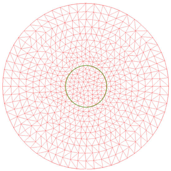
Figure 1. The domain and the mesh.

The parameters and initial data for this test are

$$T=1,y_0=x_1^2+x_2^2+100.$$

For the time discretization, we use the explicit Euler scheme with $dt=0.01$ and the P1 Lagrange for the spatial discretization. For the control function u, we select

$$u=1000·(x_1^2·x_2^2+e^{4t})+1000.$$

This setup allows us to test the algorithm under specific geometric and numerical conditions, providing insights into the behavior of the control in a circular domain. In addition, we choose the diffusion coefficients as

$$A(x_1,x_2)=\left\{\begin{array}{ccc}{A}_d\hfill & \mathrm{if}& x\in \omega ,\hfill \\ A_c\hfill & \mathrm{if}& x\in \Omega \backslash \omega .\hfill \end{array}\right.$$

being that

$$A_d=0.3A_c=1.5.$$

These two coefficients are chosen in an attempt to simulate the diffusion coefficients between the gray matter and the white matter of the human brain. The initial data, $y_0$, are taken to be big:

$$y_0(x_1,x_2)=x_1^2+x_2^2+100.$$

With all these data, if we run the program with the proposed algorithm, we find that the solution at the final time is very close to zero as can be observed in Figure 2.

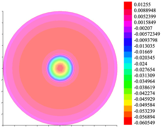
Figure 2. Solution $\widehat{y}(T)$ with $T=1$.

As can be observed, with this algorithm, we are able to achieve the solution to the null control problem at time T with discontinuous coefficients in two regions of the space.

5.2. Test 2

We now describe the second test. In this case, we consider a square domain of size $[0,6]\times [0,6]$, in which there is an interior circle with radius 2 centered at $(3,3)$, defining the control region as shown in Figure 3. The open set $\omega$ where the control acts is

$$\omega =\{(x_1,x_2)\in {\mathbf{R}}^2:{(x_1-3)}^2+{(x_2-3)}^2\le 2^2\}.$$

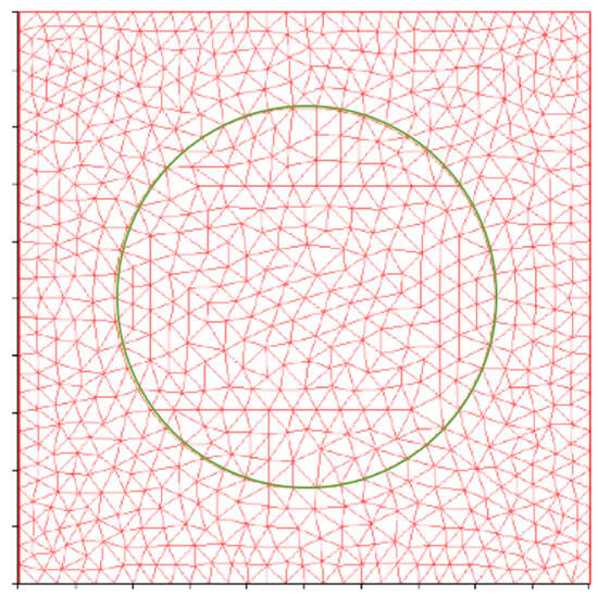
Figure 3. The domain and the control region.

For the time discretization, we use the explicit Euler scheme with $dt=0.01$ and P1 Lagrange for the spatial discretization. The initial data for this test are

$$T=3,y_0=x_1^2+x_2^2.$$

For the control function u, we select

$$u=100·x_1^2·x_2^2·e^t.$$

In this test, we create a function derived from the solution of a coupled reaction–diffusion problem, which is used to define the diffusion coefficients at each point in space as shown in Figure 4.

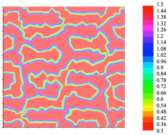
Figure 4. The diffusion coefficients at each point in space.

With all these data, if we run the program with the proposed algorithm, we find that the solution at the final time is very close to zero as can be observed in Figure 5.

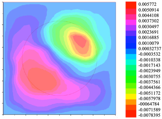
Figure 5. Solution $\widehat{y}(T)$ with $T=3$.

As can be observed, with this algorithm, we are able to achieve the solution to the null control problem at time T with discontinuous coefficients, and the solution is obtained with low computational cost.

6. Conclusions

This work provides a novel method to prove the existence of exact controls to zero at a final time, partially distributed, without relying on obtaining Carleman-type inequalities. The advantage of this approach is that it does not require regularity assumptions on the diffusion coefficients or on the boundary of the spatial domain. Thus, it extends the study of controllability to zero in finite time to cases where Carleman inequalities cannot be applied.

Furthermore, we have successfully obtained a null control with a simple and efficient algorithm that works in more general cases than those covered by traditional Carleman inequalities. This algorithm provides a practical and fast solution, demonstrating its versatility and computational efficiency.

Theorem 3 is fundamental in the proof of the control result (Theorem 5). Specifically, the theorem provides a final-time maximum principle-type result, which is of independent interest. As a consequence of the control result, a unique continuation theorem (Theorem 8) is also obtained, with the novelty that classical regularity assumptions are again not required.

This new approach to studying control problems promises significant implications, both theoretical and numerical, to be explored in future works. It is worth noting that the numerical aspect will require a dedicated investigation in a subsequent paper. This extension is far from trivial, as the current work establishes the existence of exact controls but offers a theoretical characterization rather than a straightforward algorithm for constructing such controls. However, the success of the proposed algorithm in solving the null control problem efficiently opens up new avenues for further research in this area.

References

- Lions, J.L.; Magenes, E. Problèmes aux Limites non Homogènes et Applications; Dunod: Paris, France, 1968; Volume 1. [Google Scholar]
- Swanson, K.R.; Alvord, E.C., Jr.; Murray, J.D. Dynamics of a model for brain tumors reveals a small window for therapeutic intervention; Mathematical models in cancer (Nashville, TN, 2002). Discret. Contin. Dyn. Syst. Ser. B 2004, 4, 289–295. [Google Scholar]
- Pighin, D.; Zuazua, E. Controllability under positivity constraints of semilinear heat equations. Am. Inst. Math. Sci. 2018, 8, 935–964. [Google Scholar] [CrossRef]
- Lohéac, J.; Trélat, E.; Zuazua, E. Minimal controllability time for the heat equation under unilateral state or control constraints. Math. Models Methods Appl. Sci. 2017, 27, 1587–1644. [Google Scholar] [CrossRef]
- Fernández-Cara, E.; Guerrero, S. Global Carleman inequalities for parabolic systems and applications to controllability. SIAM J. Control Optim. 2006, 45, 1399–1446. [Google Scholar] [CrossRef]
- Lebeau, G.; Robbiano, L. Controle Exacte de l’Équation de la Chaleur; (Exact Control of the Heat Equation); Semináire sur les Équations aux Derivées Partielles 1994–1995; École Polytech.: Palaiseau, France, 1995; Exp. No. VII; 13p. [Google Scholar]
- Emanuilov, Y.O. Controllabillity of parabolic equations. Sb. Math. 1995, 186, 879–900. [Google Scholar] [CrossRef]
- Benabdallah, A.; Dermenjian, Y.; Rousseau, J.L. Carleman estimates for stratified media. J. Funct. Anal. 2011, 260, 3645–3677. [Google Scholar] [CrossRef]
- Benabdallah, A.; Dermenjian, Y.; Thevenet, L. Carleman estimates for some non-smooth anisotropic media. Comm. Partial. Differ. Equ. 2013, 38, 1763–1790. [Google Scholar] [CrossRef]
- Dardé, J.; Ervedoza, S.; Morales, R. Uniform null controllability for parabolic equations with discontinuous diffusion coefficients. ESAIM Control Optim. Calc. Var. 2021, 27, 66–94. [Google Scholar] [CrossRef]
- Alessandrini, G.; Escauriaza, L. Null-controllability of one-dimensional parabolic equations. ESAIM Control Optim. Calc. Var. 2008, 14, 284–293. [Google Scholar] [CrossRef]
- Benabdallah, A.; Dermenjian, Y.; Rousseau, J.L. Carleman estimates for the one-dimensional heat equation with a discontinuous coefficient and applications to controllability and an inverse problem. J. Math. Anal. Appl. 2007, 336, 865–887. [Google Scholar] [CrossRef]
- Fernández-Cara, E.; Zuazua, E. On the null controllability of the one-dimensional heat equation with BV coefficients. Comput. Appl. Math. 2002, 21, 167–190. [Google Scholar]
- Doubova, A.; Osses, A.; Puel, J.P. Exact controllability to trajectories for semilinear heat equations with discontinuous diffusion coefficients. A tribute to J. L. Lions. ESAIM Control Optim. Calc. Var. 2002, 8, 621–661. [Google Scholar] [CrossRef]
- Mizohata, S. Unicité de prolongement des solutions pour quelques opérateurs différentiels paraboliques. Mem. Coll. Sci. Univ. Kyoto Ser. A 1958, 31, 219–239. [Google Scholar] [CrossRef]
- Ladyzenskaja, O.A.; Solonnikov, V.A.; Uralceva, N.N. Linear and Quasi-Linear Equations of Parabolic Type; American Mathematical Society: Providence, RI, USA, 1968. [Google Scholar]
- Lions, J.L. Exact controllability stabilization and perturbations for distributed systems. Rec. Math. Appl. 1988, 1, 1–68. [Google Scholar] [CrossRef]
Disclaimer/Publisher’s Note: The statements, opinions and data contained in all publications are solely those of the individual author(s) and contributor(s) and not of MDPI and/or the editor(s). MDPI and/or the editor(s) disclaim responsibility for any injury to people or property resulting from any ideas, methods, instructions or products referred to in the content. |
© 2025 by the authors. Licensee MDPI, Basel, Switzerland. This article is an open access article distributed under the terms and conditions of the Creative Commons Attribution (CC BY) license (https://creativecommons.org/licenses/by/4.0/).