Abstract
With the rapid development of global trade, the cargo throughput of automated container terminals (ACTs) has increased significantly. To meet the demands of large-scale, high-intensity, and high-efficiency ACT operations, the seamless integration of various terminal facilities has become crucial, particularly the collaboration between yard cranes (YCs) and automated guided vehicles (AGVs). Therefore, an integrated scheduling problem for YCs and AGVs (YAAISP) is proposed and formulated in this paper, considering stacking containers and bidirectional transport of AGVs. As the YAAISP is an NP-hard problem, an Improved Whale Optimization Algorithm (IWOA) is proposed in which a reverse learning strategy is used for the population to enhance population diversity; a random difference variation strategy is employed to improve individual exploration capabilities; and a nonlinear convergence factor alongside an adaptive weighting mechanism to dynamically balance global exploration and local exploitation. For container tasks of size 100, the objective function value (OFV) of the IWOA was reduced by 9.25% compared to the standard Whale Optimization Algorithm. Comparisons with other algorithms, such as the Genetic Algorithm, Particle Swarm Optimization, and Grey Wolf Optimizer, showed an OFV reduction of 9.61% to 11.75%. This validates the superiority of the proposed method.
Keywords:
automated container terminals; automated guided vehicles; yard cranes; integrated scheduling; improved Whale Optimization Algorithm MSC:
68T20
1. Introduction
The automated container terminal (ACT) is a key hub in the global supply chain network. With the rapid development of global economic trade and the increase in the size of ships, the volume of shipping orders has soared. This surge poses significant challenges to the transfer capacity and service levels of container terminals. The number of mega-ships and containers worldwide is expected to continue to grow in the future. Improving the efficiency of container terminals can help reduce operational energy consumption and costs, enhance customer satisfaction, and maintain a competitive edge in a highly competitive industry. Technologies such as the Internet of Things, automation, and artificial intelligence have been well-applied in the shipping industry to enhance safety, efficiency, and sustainability during goods transportation [1]. Currently, most container terminals employ advanced automation equipment, such as quay cranes (QCs), yard cranes (YCs), and automated guided vehicles (AGVs). However, the high cost of these new loading, unloading, and transportation equipment means that their resources are limited. Therefore, reasonable and coordinated scheduling of this equipment is crucial for maintaining the service levels of ACTs [2].
In this context, ACTs are presented with new opportunities to meet the high service standards demanded by stakeholders, such as freight forwarders, logistics companies, and shipping operators. Some container terminals have been innovated in technology, management, organization, and culture to seize these opportunities [3]. Many previous studies have divided the field of ACTs into several independent blocks, which are then subdivided into different problems to study. These subproblems include YC scheduling, AGV scheduling and path planning, QC scheduling, ship berth allocation [4]. However, since the operations of different equipment are interrelated, it is unreasonable to deal with resources separately. This will result in significant mutual waiting times among equipment. Therefore, the integrated scheduling of ACT equipment is now the mainstream research problem. In an ACT, efficiency depends primarily on the synchronization of AGVs and YCs. In many existing studies in the literature, AGV and YC scheduling are mostly considered independently. Therefore, this paper focuses on the integrated scheduling problem of AGVs and YCs (YAAISP).
However, the complexity of the YAAISP is NP-hard. This means that as the problem size increases, the solution time will grow exponentially, and the algorithm will face the curse of dimensionality as the problem’s dimensions increase. In recent years, the application of metaheuristic algorithms in solving complex optimization problems has gained widespread attention because they can find approximate optimal solutions in polynomial time, unlike traditional methods that require exponential computation time. Various metaheuristic algorithms and their variations have been successfully applied to many scheduling fields, including port scheduling. According to the latest review, swarm intelligence algorithms, such as the Genetic Algorithm (GA), Grey Wolf Optimizer (GWO), and Particle Swarm Optimization (PSO), have been widely applied to optimization problems in ACT scheduling.
The Whale Optimization Algorithm (WOA), an emerging metaheuristic algorithm inspired by the bubble-net hunting behavior of humpback whales, was proposed by Mirjalili and Lewis [5]. It features a simple search strategy, minimal parameter requirements, and robust search capabilities. Unlike classical algorithms, such as GA, PSO, and GWO, WOA uniquely balances exploration and exploitation by dynamically adjusting key parameters during the iteration process. This adaptability has led to its widespread application across various engineering domains [6,7,8]. In the context of integrated scheduling optimization, particularly for ACTs or similarly complex scheduling challenges, traditional methods often struggle to efficiently manage multiple tasks while achieving global optimization under intricate constraints. This paper investigates the application of the WOA in ACT scheduling optimization, with a focus on minimizing task completion times—a critical factor for ensuring the seamless coordination of YCs and AGVs. By mapping task scheduling to the whale-foraging model, WOA is employed to approximate optimal solutions. To further enhance its performance, this study introduces an Improved Whale Optimization Algorithm (IWOA), which improves the search capabilities of the original WOA. Extensive simulation experiments are conducted to evaluate the effectiveness of the IWOA, demonstrating its potential as a powerful tool for port scheduling. The main contributions of this paper are as follows:
- A more comprehensive model for the YAAISP is proposed in this paper, in which AGVs’ bi-directional flow, coordinated operations of import and export container tasks, and container task constraints relationship are considered simultaneously.
- A specific encoding and decoding method is developed for the YAAISP, ensuring the feasibility of all encoding schemes without the need for adjustments or discarding, expanding the search space for potential solutions.
- An IWOA algorithm is proposed to solve the YAAISP, and population initialization with inverse learning and a random differential mutation strategy are implemented to enhance the diversity of solutions, effectively preventing the algorithm from getting trapped in local optima. The nonlinear convergence factor and adaptive weight strategy are used to dynamically adjust the weights, thereby accelerating the convergence speed of the algorithm.
The rest of this article is organized as follows. Section 2 reviews the relevant literature. In Section 3, the YAAISP is described, and the problem is formulated as an MIP model. In Section 4, an IWOA is proposed to solve the YAAISP presented in this study. Section 5 shows and analyzes the numerical results to validate the correctness of the formula model and the superiority of the proposed algorithm. In Section 6, the conclusions are given and suggestions for further research are put forward.
2. Literature Review
In recent years, with the continuous development and expansion of ACT trade, the operation and scheduling of intelligent terminal equipment have been extensively studied. For traditional container terminals, numerous studies have focused on the scheduling of YCs, QCs and AGVs. Among these, the impact of QCs is the least significant because the buffer on the QCs’ side decouples the QCs from the AGVs. This section reviews the research on YC scheduling, AGV scheduling, and the integrated scheduling to identify gaps in the existing literature.
2.1. YC Scheduling Problem
In the field of research on YCs, most researchers primarily focus on aspects related to the static scheduling and dynamic scheduling of YCs.
In the context of static scheduling, most researchers have considered the issue of interference between dual YCs. For example, Ng [9] studied the interference generated by multiple cranes and lanes, considered the safe distance between YCs, and developed a heuristic algorithm to solve the YC scheduling problem. Saini, Roy, and De Koster [10] constructed a two-level random model to analyze the performance of dual YCs. It was found that the interference effect between cranes would reduce the handling capacity of cranes by about 35%, and the interference delay increases with the number of shelves in the stack. Zheng et al. [11] believed that in the crane scheduling problem of the double yard with inter-crane interference constraints, the task processing time would change dynamically because of the arrangement of the task retrieval and storage. Additionally, many studies focus on the storage and stacking of containers. L. Chen and Langevin [12] studied the movement of the YC among the container blocks and the order of the YC in each stack and proposed a GA and a tabu search algorithm to obtain the approximately optimal solution. Galle and Jaillet [13] considered the YC scheduling problem, and the container relocation problem expressed this problem as an MIP model and solved it with a solver. They developed a heuristic, called dividing, sequencing, and comparing, and a GA based on the characteristics of the problem.
In the field of the dynamic scheduling of YCs, He et al. [14] established a YC dynamic scheduling model based on goal programming and adopted a hybrid algorithm of heuristic rules and a parallel genetic algorithm to solve the problem. L. He, Tan, and Zhang [15] solves a YC scheduling problem with uncertainty about the arrival time and processing volume of the task group. A mathematical model is proposed to optimize the total delay and additional loss of the estimated end time for all task groups under the scenarios of no uncertainty and all uncertainties. In addition, a GA-based framework combining a three-stage algorithm is proposed to solve this problem. Li et al. [16] considered the flexible scheduling of double YCs in container terminals with a dynamic cut-off time. To solve this problem faster and more effectively, the integrated scheduling of PSO and local rescheduling strategy was proposed to solve this problem. Liu et al. [17] proposed a flexible YC scheduling model that optimizes the mixed operations of railway and road containers through a two-stage approach.
2.2. AGV Scheduling Problem
In the current research field of AGV scheduling, numerous scholars have proposed various methods and addressed different problems. Based on the core research focus, these studies can generally be categorized into the static scheduling of AGVs and the dynamic scheduling of AGVs in complex environments.
In the field of AGV static scheduling, Kim and Bae [18] proposed a look-ahead dispatching method for AGVs to reduce delays in ship operations. Rashidi and Tsang [19] solved the scheduling problem of AGVs by designing an extended Network Simplex Algorithm and developed the minimum-cost flow model. To minimize a ship’s berthing time, Luo and Wu [20] proposed a new method that considers both AGV scheduling rules and container storage locations for unloading and loading processes and used genetic algorithms to solve large-sized problems. Ma, Bian, and Gao [21] proposed an algorithm based on priority rules, called the shuffle Leapfrog algorithm, which has an abrupt process, to solve the multi-load AGV scheduling problem of ACTs.
In the field of the dynamic scheduling of AGVs, Angeloudis and Bell [22] introduced an innovative algorithm based on a cost/benefit approach to address the AGV dispatching problem in uncertain terminal environments, particularly focusing on the unpredictable task durations of future events. Xu et al. [23] proposed a response-based scheduling strategy for AGVs, utilizing a “request-scheduling-response” model to tackle dynamic logistics scheduling in intelligent manufacturing workshops, with the goal of minimizing both the completion time and the required number of AGVs. Dang et al. [24] examined the scheduling challenges of heterogeneous multi-load AGVs under battery limitations, developing an MIP model and a hybrid algorithm combining adaptive large neighborhood search to solve the issue. To address the complexities of AGV scheduling in smart factory material handling, L. Zhang et al. [25] created a dynamic scheduling approach for self-organizing AGVs, aiming to reduce delays and optimize logistics costs. Li et al. [26] proposed a solution using Curriculum Learning and the Multi-Feature Fusion Transformer to maintain high prediction accuracy in electric vehicle charging monitoring systems, even with 90% of the data missing. Aljanabi and Borna [27] developed a model combining singular value decomposition, GA, and adaptive neuro-fuzzy inference system to optimize transportation costs and CO2 emissions in port-based multimodal transport, achieving improved efficiency and accuracy. Shao et al. [28] proposed an AGV delivery-route optimization method based on a rolling scheduling framework, embedding a stochastic programming model to address dynamic demand and uncertainties.
2.3. Integrated Scheduling Problem
There is relatively little literature on the integrated scheduling of YCs and AGVs. X. Zhang, Gu, and Tian [29] studied the integrated scheduling optimization of AGVs and YCs, considering the impact of different charging strategies on AGV scheduling under charging constraints. Zhou, Lee, and Li [30] presented a comprehensive optimization method to simultaneously determine the yard crane schedule and vehicle parking location under Chebyshev movement to allow the gantry frame of the yard crane and the trolley to move simultaneously. An MIP model is formulated to optimize the problem, and the two-stage heuristic algorithm is developed to solve the problem efficiently. Q. Zhang et al. [31] established an integrated scheduling model of AGVs and YCs in ACTs’ relay operation mode considering the buffer capacity constraints and dual YC operation interference and solved it using GA. Chen et al. [32] studied the YC and AGV scheduling problem based on extended space–time networks and modeled the problem using the idea of multi-population network flow, which was solved by the alternate direction method of the multiplier. By considering the coordination between AGVs and yard cranes, as well as the interference between double yard cranes, X. Zhang, Li, and Sheu [33] propose a hybrid integer programming model with the goal of minimizing the completion time and the design of a branch and binding algorithm based on PSO to solve the model. Luo, Wu, and Mendes [34] provided an integrated modeling approach to solve two key problems, AGVs/YC scheduling and container storage, which was described as an MIP model, and they also developed a specialized approach to novel designs based on genetic algorithms. Ma et al. [35] proposed a hybrid speed optimization strategy and a mixed-integer time-energy coordinated scheduling model based on the Chaotic Inverse Learning-Based Slime-Mold Genetic Algorithm, which significantly improves the operational efficiency of the container terminal by optimizing AGV and yard crane scheduling.
However, most of these studies have not fully considered the container transfer process, specifically transporting both import and export container tasks simultaneously. Additionally, within container tasks, there may be situations where one container task must be executed before another because of stacking or other constraints, indicating the presence of priority relationships among tasks. This factor has also not been adequately considered. While such simplifications may simplify the problem, they do not reflect the realities of terminal operations. This paper considers these factors in the integrated scheduling process of YCs and AGVs.
3. Problem Description and Formulation
3.1. Problem Statement
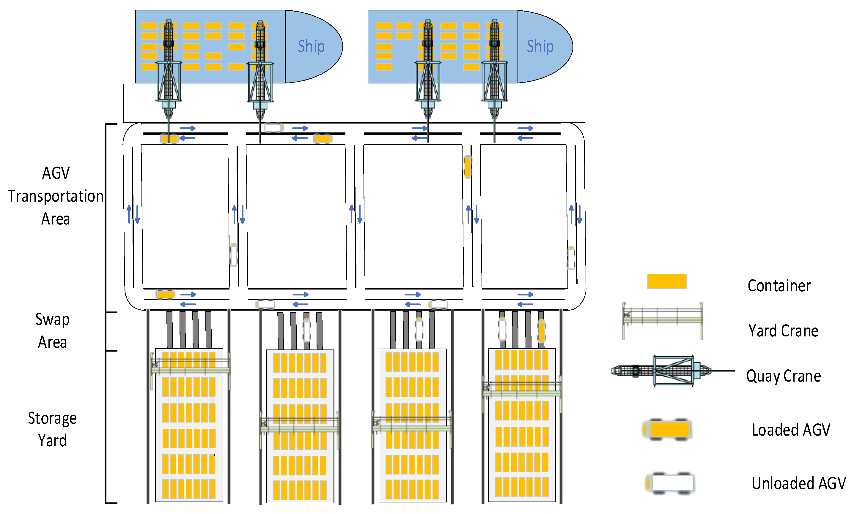
In the operations of ACTs, when a container ship berths, a complex bidirectional flow process occurs involving the handling of both import and export containers. Import containers from the ship need to be transported by AGVs from the quayside to the yard side for storage using YCs. Simultaneously, export containers from the yard must be loaded onto AGVs by YCs and then transported to the quayside for loading onto the ship. In traditional terminal operations, YCs handle container tasks within the current yard, and AGVs are allocated to serve specific YCs. In this method, each working YC cooperates with a fixed group of AGVs, which often leads to mutual waiting times between YCs and AGVs, resulting in low terminal efficiency (see Figure 1).
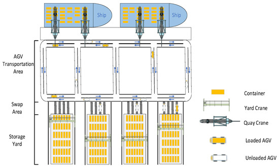
Figure 1.
The layout of an automated container terminal.
In this paper, an integrated scheduling approach for YCs and AGVs is proposed, where YCs are not assigned fixed AGVs. Instead, the number of tasks for AGVs and the YCs they serve are dynamically adjusted to minimize the make-span of the ACTs. During integrated scheduling, the scheduling of YCs must consider the constraint relationships between container tasks to generate a reasonable sequence. The scheduling of AGVs involves assigning container tasks to AGVs, and the sequence of AGV tasks is constrained by the scheduling order of YCs.
3.2. Notations
This section describes the definitions of some indices, parameters, and variables used in the mathematical model, as shown in Table 1.

Table 1.
Sets and parameters.
3.3. Assumptions
There are some reasonable assumptions that help solve the integrated scheduling problem:
- The loading and unloading points for all container tasks are known;
- The initial positions of the AGVs are known;
- Each AGV can only transport one container task at a time;
- Each container task can only be assigned to one AGV at a time;
- The working time of YCs processing a container task is evenly distributed between (40, 60);
- The efficiency of QCs is high enough to ignore the time of QCs handling container tasks;
- The constraints relationship between each container task is known, and the lower container must wait for the upper container to move before it can be operated.
3.4. Mathematical Modeling
This section describes the definitions of some indices, parameters, and variables used in the mathematical model, as shown in Table 1. Based on the above assumptions and notations, we formulated the problem as the following mathematical model:
The objective of Function (1) is to minimize the maximum completion time. Function (2)’s objective is to take the maximums of the AGVs’ completion time and the YCs’ completion time.
This is subject to the following:
Constraint (3) specifies that the start time of YC y’s current container task should be equal to the end time of the previous task.
Constraint (4) states that the time at which the AGV arrives at the loading point for current export container task i should be equal to the time at which the AGV completes the previous container task j plus the travel time required to move from the unloading point of the previous container task j to the loading point of the current container task i.
Constraint (5) represents the temporal relationship between the start time of export container task i by YC y and the completion time of the previous container task j handled by the same YC y.
Constraint (6) indicates that the completion time of YC y to process export container task i should be equal to the maximum value between the time when the AGV arrives at container task i and the start time at which YC y processes task i plus the time required to process task i.
Constraint (7) indicates that the time for the AGV to start transporting export container task i is equal to the time for YC y to complete container task i.
Constraint (8) indicates that the time for the AGV to complete the export container task i is equal to the time for the AGV to start the transportation task i plus the time for the task i to go from the loading point to the unloading point.
Constraints (4) to (8) are for export container tasks handled by YCs and AGVs.
Constraint (9) indicates that the start time of the AGV processing the current import container task i is equal to the end time of the AGV processing the previous container task j plus the time required to travel from the unloading point of task j to the loading point of the current import container task i.
Constraint (10) states that the arrival time of the AGV transporting the import container task i is equal to the start time of the AGV processing container task i plus the time required to travel from the loading point to the unloading point of the current container task i.
Constraint (11) indicates the temporal relationship between the start time of YC y processing import container task i and the completion time of the previous container task j handled by YC y, as well as the time when the AGV arrives at the location of unloading point of task i.
Constraint (12) indicates that the completion time of YC y processing import container task i is equal to the start time of YC y processing import container task i plus the operation time of processing container task i.
Constraint (13) indicates that the time for the AGV to complete import container task i is equal to the time for YC y to start processing import container task i.
Constraints (9) to (13) are constraints on the handling of import container tasks by YCs and AGVs.
Constraint (14) guarantees that if tasks i and j belong to the set , task i must precede task j in the handling process.
Constraint (15) ensure that if tasks i and j belong to set , the two tasks cannot be performed simultaneously.
Constraints (16) and (17) define the binary variable . is equal to 1 in the case that task j must be handled after the operation of task i, and is equal to 0 in the case that task i started after the completion of task j.
Constraints (18) and (19) guarantee that each YC starts at its initial state, O, and ends at its final state, F, respectively.
Constraints (20) and (21) guarantee that each AGV starts at its initial state, O, and ends at its final state, F, respectively.
Constraint (22) constructs a flow balance for each YC.
Constraint (23) constructs a flow balance for all AGVs.
Constraint (24) states that each container task is assigned to one and only one truck.
Constraint (25) and Constraint (26) show that any two successive tasks of YCs and AGVs cannot have a conflicting sequential order.
Constraint (27) restrict the domains of the decision variables.
4. IWOA Algorithm for YAAISP
This section first introduces the solution’s representation in Section 4.1, which is applicable to both the standard WOA and the proposed IWOA. Section 4.2 presents the standard WOA. Finally, Section 4.3 introduces improvement strategies based on the standard WOA.
4.1. Solution Representation
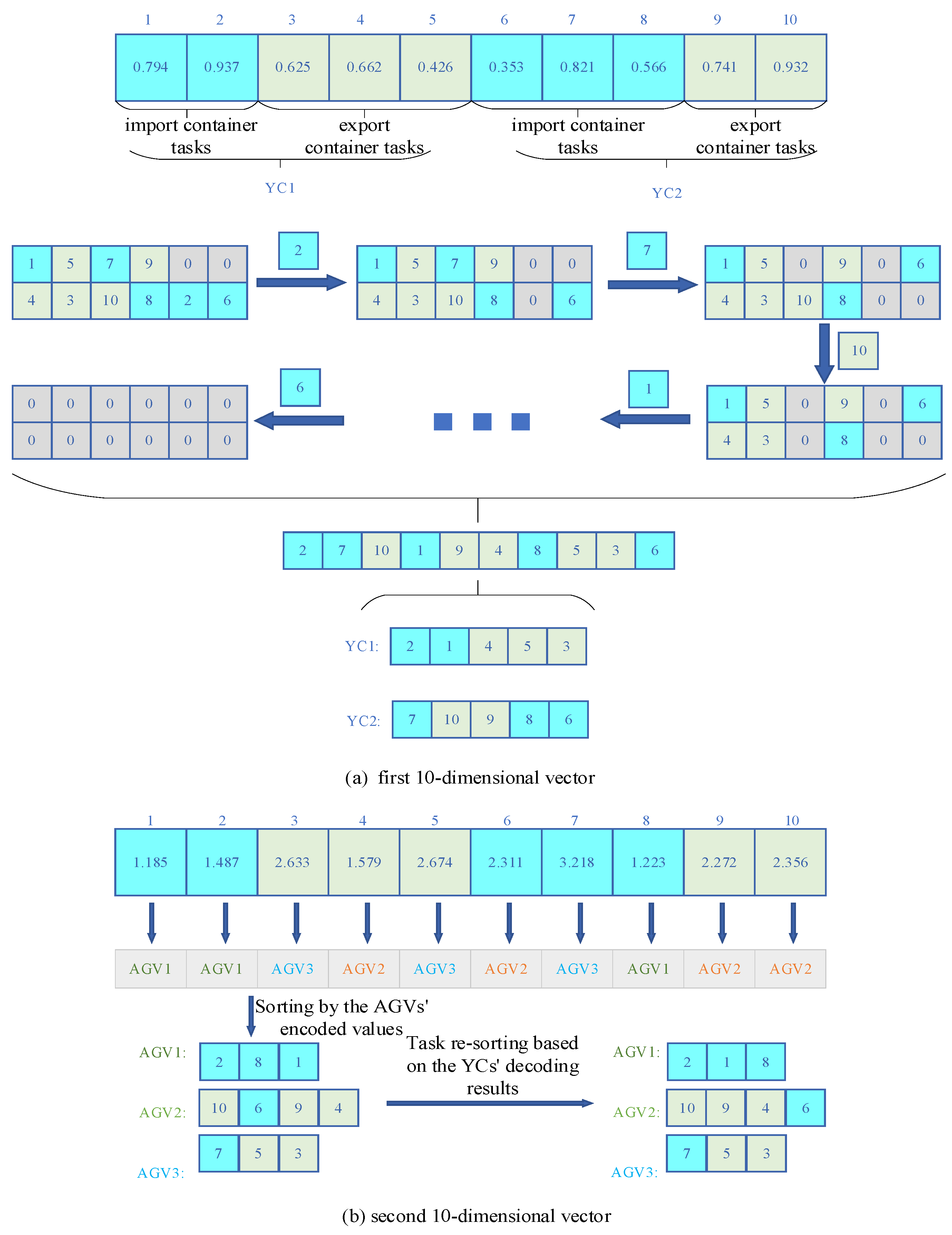
A 2M-dimensional vector is used to represent the solution for the YAAISP, where M is equal to the number of container tasks. Given that , where represents the number of YCs. The encoding method adopted in this paper is that of random numbers. The range of random numbers encoded in the first M-dimensional vector is [0, 1], and the range of random numbers encoded in the second M-dimensional vector is [0.5, + 0.5], where represents the number of AGVs, and the number above each dimension represents the task number of the container.
Consider a system with two YCs and three AGVs handling 10 container tasks, where the encoding length is 20. In this example, the decoding process of the first 10-dimensional vector accounts for the constraints between the container tasks. To illustrate these relationships more clearly, the constraints can be represented in a matrix. In this matrix, container tasks with constraints are placed in the same column, with tasks having higher encoded values positioned above the current column. Tasks without constraints are placed in separate columns, and empty positions are filled with 0.
As shown in subfigure (a) of Figure 2, the constraints between container tasks are (1, 4), (5, 3), (7, 10), and (9, 8). The non-0 container tasks on the top level are 1, 5, 7, 9, 2, and 6, and in the first 10-dimensional vector, 1, 5, 7, 9, 2, and 6 have values of 0.794, 0.426, 0.821, 0.741, 0.937, and 0.821, respectively. Therefore, container task 2 has the largest value, so YC executes container task 2 first. After removing container task 2 from the matrix, the value at the position of container task 2 is replaced with 0. The remaining top layer includes container tasks 1, 5, 7, 9, and 6. The random number encoding values for tasks 15, 7, 9, and 6 are then compared. The maximum value is 0.821, which is container task 7. Then, container task 7 is removed from the matrix, etc., and the final order of the YC scheduling is 2, 7, 10, 1, 9, 4, 8, 5, 3, and 6. Since tasks 1, 2, 3, 4, and 5 belong to YC1, and tasks 6, 7, 8, 9, and 10 belong to YC2, the scheduling sequences for YC1 and YC2 are 2, 1, 4, 5, 3, and 7, 10, 9, 8, and 6, respectively.

Figure 2.
Encoding and decoding process diagram.
As shown in subfigure (b) of Figure 2, the second 10-dimensional vector encoded assigns tasks to the AGV. Taking the first code of the second 10dimensional vector encoded as an example, 1.185 is between the intervals [0.5, 0.5 + 1], rounded to 1. Therefore, container task 1 is assigned to AGV1. In the same way, tasks at other locations are assigned separately to different AGVs. Finally, the tasks of AGV1 are 2, 1, and 8, the tasks of AGV2 are 10, 6, 9, and 4, and the tasks of AGV3 are 7, 5, and 3. However, the execution sequence of the AGV tasks should follow the scheduling sequence of the YCs. Therefore, the task order of the AGVs is re-sorted through the scheduling order of the YCs. After re-sorting, the task order of AGV1 is 2, 8, and 1. The AGV2 task sequence is 10, 9, 4, and 6. AGV3’s task sequence is 7, 5, and 3.
At this point, an integrated scheduling solution for the YCs and AGVs is presented.
4.2. Standard WOA Algorithm
The WOA algorithm is inspired by the foraging behavior of humpback whales. After discovering prey, humpback whales approach the prey in a spiral motion, circling around it while releasing a bubble net for hunting. The whale’s foraging behavior involves three methods: encircling prey, bubble-net attacking, and searching for prey. The following are detailed descriptions of these three methods:
- Encircling prey
Search agents explore the global space to locate and surround the optimal solution. The current best candidate is treated as the target prey. Other agents update their positions towards this best candidate. The mathematical model of this process is as follows:
where is the local optimal solution, is the position of the individual vector, and t is the number of current iterations. and are coefficient vectors, and the mathematical expressions of and are as follows:
where the vector decreases linearly from 2 to 0, is a random coefficient vector in the range [0, 1], and itermax represents the maximum number of iterations.
- Bubble-net attacking
Whales also attack their prey through a bubble-net strategy, which includes both shrinking around and spiral updates. When −1 < A < 1, the search agent contracts towards the best whale in the current situation, updating the whale group’s location according to Equation (29). As they move in a shrinking circle, whales use a spiral motion to swim towards their prey, as described below:
where represents the absolute value for the distance between the current whale and the best positioned whale; q is a constant representing the shape of the spiral; and l is a random number belonging in the range [−1, 1]. Whales either spiral around or shrink their circle with a 50% probability of updating their positions. The mathematical model of the behavior is described as follows:
where p is the random number between [0, 1].
- Hunting for prey
In the WOA, parameter A controls the whale hunting behavior. When |A| ≥ 1, whales explore by moving towards a random whale.
where is the position vector of the randomly selected whale.
4.3. Proposed IWOA Algorithm
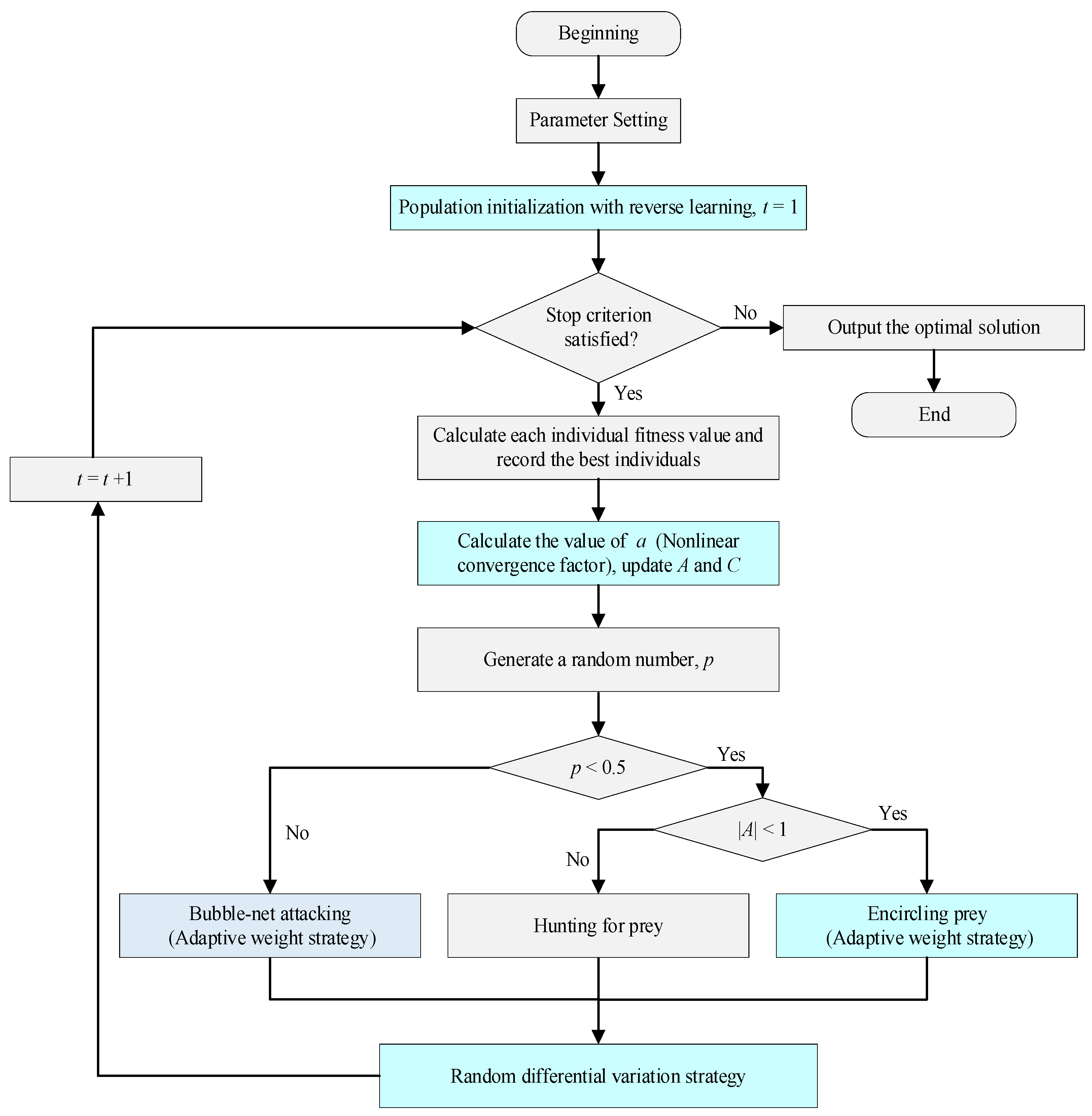
The standard WOA suffers from a slow convergence speed and a tendency to fall into the local optima. To address these shortcomings, the IWOA introduces the following key improvements: population initialization with reverse learning and random difference mutation strategies to prevent the algorithm from getting trapped in the local optima, as well as nonlinear convergence factors combined with adaptive weight strategies to dynamically adjust the search process and enhance the convergence speed. A flowchart of the IWOA is presented in Figure 3, with the blue sections highlighting the improvements over the standard WOA.
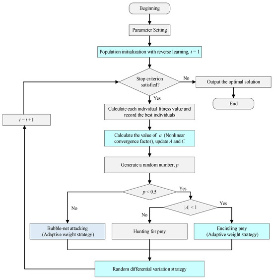
Figure 3.
IWOA flowchart.
The computational complexity of the IWOA is primarily influenced by the population size (N), problem dimension (D), number of iterations (T), and complexity of the fitness function (Cf). During the population initialization phase, the complexity arises from generating the initial and reverse populations O (2N × D), evaluating the fitness of all individuals O (2N × Cf), and selecting the top N individuals O (2Nlog(2N)). Thus, the total complexity for initialization is O (2N × D + 2N × Cf + 2Nlog2N). In the position update phase, the complexity includes updating the position of each individual O (N × D), applying random differential mutation O (N × D), evaluating the fitness of all individuals O (2N × Cf), and selecting the best individuals O (2Nlog(2N)), resulting in a total complexity of O (2N × D + 2N × Cf + 2Nlog(2N)). For the iteration phase, the overall complexity becomes O (T × (2N × D + 2N × Cf + 2Nlog(2N))), where T is the number of iterations. Combining all phases, the total computational complexity of the IWOA is O (2N × D + 2N × Cf + 2Nlog2N) + O (T × (2N × D + 2N × Cf + 2Nlog(2N))).
- Population initialization with reverse learning
The standard WOA algorithm utilizes random initialization, which often results in high randomness and does not guarantee sufficient diversity in the initial population. To address this, an enhanced approach using reverse learning is introduced for population initialization. Reverse learning involves defining the variable’s boundary range and deriving its corresponding reverse solution based on specific rules, thereby ensuring greater diversity in the initial population.
In the WOA, assuming the size of the population is N and the search space is 2M-dimensional, the position of the i-th whale in the 2M-dimensional can be expressed as follows: , , , and are the lower and upper limits of , respectively. The inverse solution corresponding to is shown in Equation (38):
When N individuals of the algorithm population are initialized, N reverse individuals are created, and each reverse individual corresponds to one of the N initial individuals. Given 2N candidate solutions (N initial individuals and N reversals), the best N is reserved as the population where the reverse evolution algorithm starts. Each inverse of N individuals is calculated every one generation, and among these 2N candidate solutions, the best N individuals are reserved for the next generation. This not only ensures the diversity of the population but also enables the population to converge quickly to the global appropriately optimal solution. The formula for selecting N better individuals is as follows:
where fitness is the fitness function, and present randomly generated individual and reverse learning individuals, respectively.
- Nonlinear convergence factor
Similar to other swarm intelligence optimization algorithms, the WOA also faces the challenge of balancing global exploration and local exploitation during the optimization process. In the standard WOA, this balance is controlled by the parameter |A|. When |A| ≥ 1, the algorithm conducts a random global search with a 50% probability, whereas for |A| < 1, it emphasizes local exploitation. However, the linear variation in convergence parameter a proves inadequate for effectively regulating this balance. To address this limitation, this paper introduces a nonlinear convergence factor, defined as follows:
Equation in the WOA is improved to:
- Adaptive weight and random differential mutation strategy
This paper employs an exponentially changing adaptive weight method. During the early iterations, the algorithm uses a large weight to achieve strong global search performance and ensure the search range. As the iterations progress, the weight value decreases exponentially, improving the algorithm’s local optimization performance as it approaches the near-optimal solution. The adaptive weight strategy is employed to update individual positions during encircling prey or bubble-net attacking behavior. The adaptive weight formula is provided in Equation (41), while the improved position update formulas are presented in Equations (42) and (43):
Equation (29) in the WOA is improved to:
Equation (33) in the WOA is improved to:
After updating the position of each individual using the adaptive weight strategy, a further update is performed through the random differential mutation strategy. The better fitness value between the pre- and post-mutation positions is retained. This approach accelerates population convergence and effectively prevents the algorithm from falling into local optima. The synergy between these two strategies enables the population to achieve superior optimization results. The random differential mutation strategy is presented in Equation (44):
where and are random numbers between [0, 1], and is the randomly selected individual in the population.
5. Validation and Results Analysis
In this section, Section 5.1 first explains the generation of the instance. Then, the algorithm parameters are set in Section 5.2. Additionally, a large number of comparative experiments are conducted in Section 5.3 to verify the effectiveness and superiority of the IWOA algorithm, and the experimental results are analyzed and discussed. We implemented all algorithms and experiments on a computer running the Windows 11 operating system with a 2.30 i7-12700 GHz Intel (R) Core (Tm) CPU and 16 GB of RAM.
5.1. Instance Generation
The ACTs studied in this paper are equipped with four YCs and four QCs in the yard and the shore block, respectively. The number of available AGVs ranges from 3 to 15, traveling at a speed of 5 m/s. The efficiency of QCs is high enough to ignore the working hours of QCs. The considered number of loading and unloading containers varies from 4 to 100, where 4–24 is considered for small-sized problems and 25–100 for large-sized problems, and the operation time of a single container task through the YC obeys a discrete uniform distribution (40, 60).
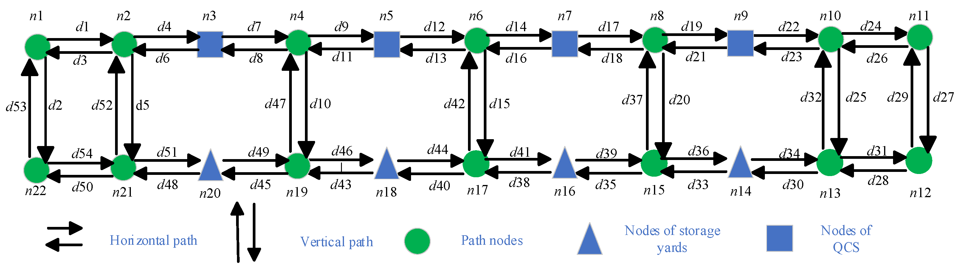
To better describe the scheduling problem of AGVs, the transportation area of AGVs is shown in Figure 1, which can be described as a weighted directed graph. As shown in Figure 4, n3, n5, n7, and n9 represent the following four nodes in the QCs: QC4, QC3, QC2, and QC1, respectively, and n14, n16, n18, and n20 represent the following four nodes in the YCs: YC4, YC3, YC2, and YC1, respectively. The other nodes are path nodes. The length of the horizontal path is 50 m, and the length of the vertical path is 75 m. This paper uses the Dijkstra algorithm to calculate the shortest distance between the starting and ending points of each container task transported by the AGVs through a weighted directed graph. The transit time required for each container task is obtained by dividing the calculated shortest distance by the speed.

Figure 4.
Weighted directed digraph of the AGVs’ transportation area.
5.2. Parameter Setting
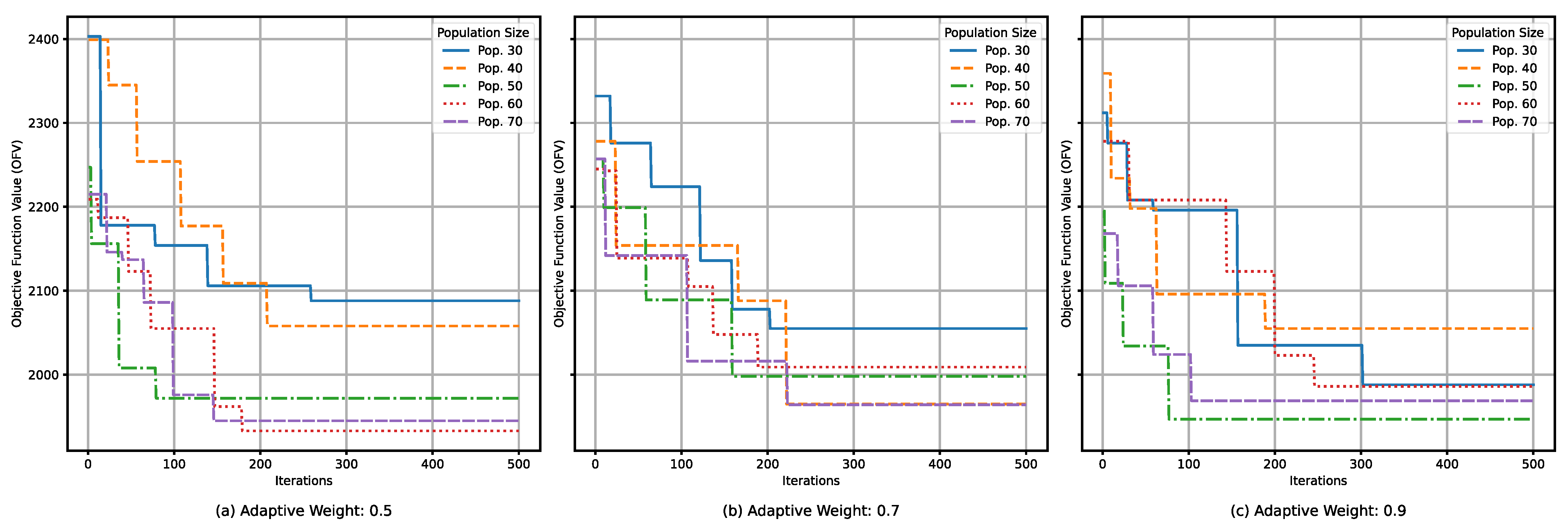
Figure 5 illustrates the impact of the adaptive weight coefficient, w, and the population size, popSize, on the solving performance of the IWOA under the following specific conditions: 80 tasks, 4 YCs, 4 QCs, 10 AGVs, and 500 iterations. The tested settings include the popSize = {30, 40, 50, 60, 70} and w = {0.5, 0.7, 0.9}. As shown in Figure 5 and Table 2, the algorithm achieves higher-quality solutions within shorter timeframes when w = 0.9 and popSize = 50. Additionally, the algorithm generally converges after approximately 300 iterations. Based on these findings, this paper set the number of iterations for the IWOA = 300, w = 0.9, and popSize = 50.
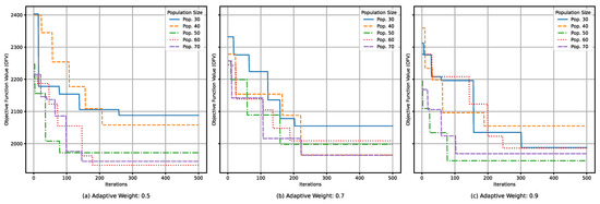
Figure 5.
Effects of changing the parameters in the IWOA.
Table 2.
CPU runtime under different parameters.
The parameter settings for other algorithms in related fields were referenced [33,36,37], and all algorithms were tested on the same problem instances and under identical initial conditions. Each algorithm underwent parameter tuning through cross-validation and experimental testing to determine the approximately optimal parameters, ensuring the fairness of the comparison. Specifically, the crossover rate, Pc, of the GA was set to 0.9, and the mutation rate, Pm, was set to 0.1. The parameters for the GWO include a convergence factor, a, which decreases linearly from 2 to 0, and random vector coefficients, r1 and r2, between [0, 1]. The parameters for the PSO include an inertia weight, h, of 0.7; cognitive weight, c1, of 1.5; and social weight, c2, of 1.5. The popSize for all algorithms was set to 50, and the maximum number of iterations was 300. Each experiment was repeated 10 times, and the average value was taken to reduce the impact of outlier results.
5.3. Results and Analysis
To verify the effectiveness of the integrated scheduling method, the CPLEX solver was used to solve the integrated scheduling problem, and the results of the CPLEX are compared with the integrated and non-integrated scheduling solutions of the IWOA. In non-integrated scheduling, the AGVs are assigned to the fixed YCs, meaning each AGV exclusively serves a specific YC. In the case of integrated scheduling, the AGVs dynamically provide services to the YC. Data from 15 experiments, with the number of container tasks ranging from 4 to 24, are summarized in Table 3. As can be seen from Table 3, the IWOA can quickly solve problems in a short time, while the CPLEX solver’s solution time becomes extremely large with the increase of problem size, and it cannot quickly solve problems in a reasonable time. Moreover, the experimental results demonstrate that, compared with non-integrated scheduling, the GAP between the objective function value (OFV) of the integrated scheduling and the CPLEX solver is smaller, and the solution time is shorter. This confirms the superiority of the integrated scheduling method. The formula for calculating GAP1 and GAP2 is shown in Equations (45) and (46), as follows:
where OFVNIS (IWOA) and OFV IS (IWOA) denote the OFVs of the non-integrated and integrated scheduling under the IWOA algorithm, and OFVIS (CPLEX) represents the OFV of the integrated scheduling under the CPLEX solver.
Table 3.
Comparison of the integrated and non-integrated solutions.
To verify the stability and effectiveness of the improvement strategy, the OFVs of the WOA and IWOA were compared. GAP3, which measures the relative percentage improvement of the IWOA over the WOA, was calculated for the same set of experiments. A larger GAP3 indicates a greater improvement in the algorithm’s performance. The formula for calculating GAP3 is shown in Equation (47), as follows:
where OFVIS (WOA) and OFVIS (IWOA) denote the OFVs obtained by the WOA and IWOA under integrated scheduling, respectively.
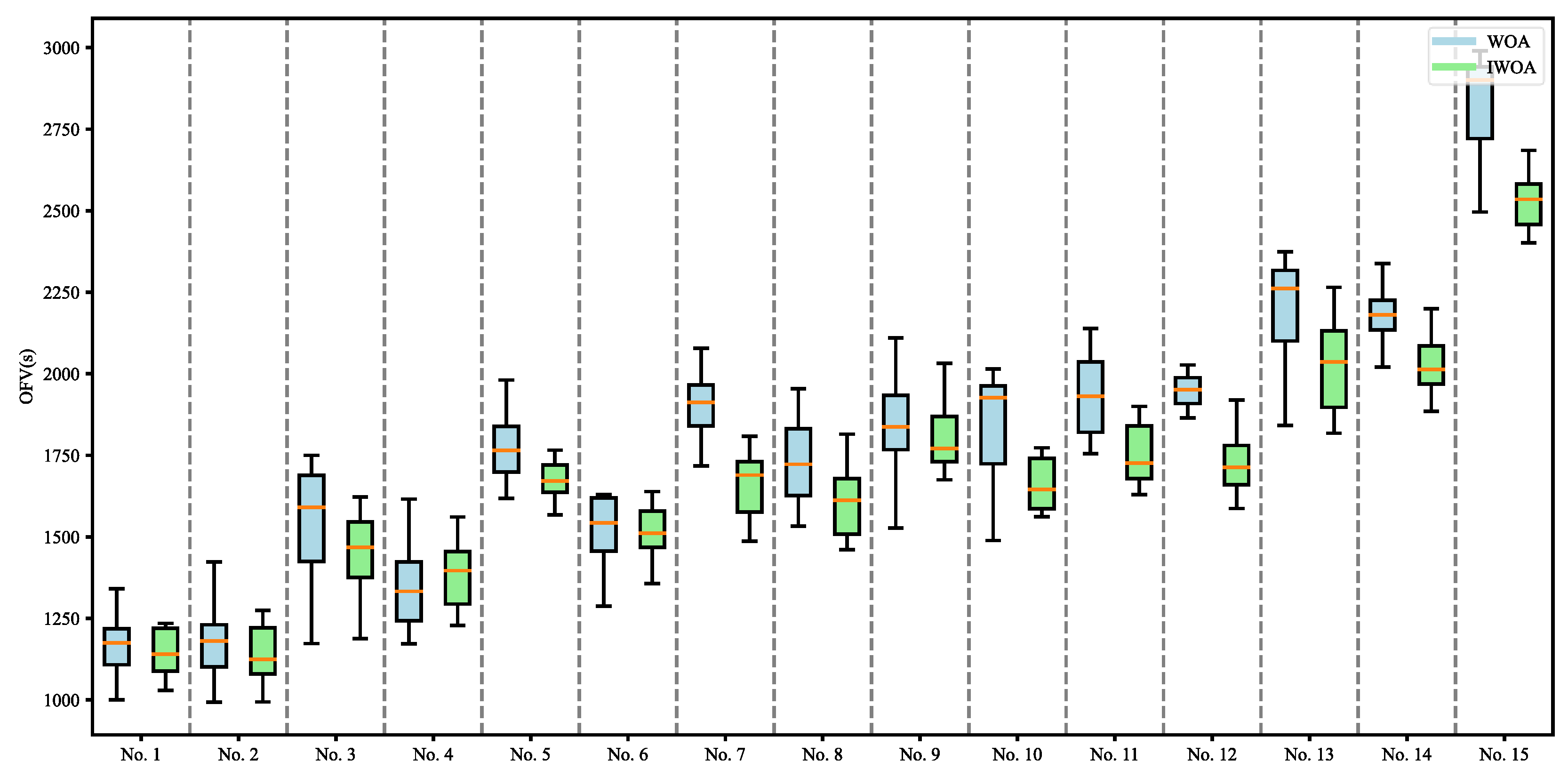
The experimental results are shown in Table 4 and Figure 6. In the 15 experiments summarized in Table 4, the OFVs of the WOA ranged from 1211 to 2550, while those of the IWOA ranged from 1135 to 2314. The lower and upper bounds of GAP3 between the WOA and the IWOA were 3.64% and 9.25%, respectively, with an average GAP3 of 6.62%. Figure 6 shows a boxplot based on the data from the 15 experiments in Table 4, with each experiment repeated 10 times. The results indicate that, in most cases, the upper and lower bounds of the solutions obtained by the IWOA were significantly lower than those of the WOA. Furthermore, the narrower solutions range of the IWOA demonstrates a higher quality of solutions, confirming the effectiveness of the proposed improvement strategies for the IWOA.
Table 4.
Comparison between the WOA and IWOA under the integrated scheduling.
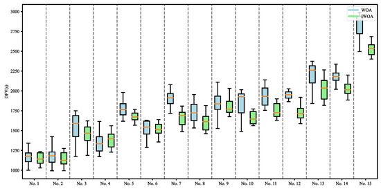
Figure 6.
The distribution of solutions in the 15 groups in Table 4.
To demonstrate the superiority of the IWOA, the OFVs obtained by the IWOA algorithm were compared with those produced by other algorithms, including GA, GWO, and PSO. The experimental results, presented in Table 5, show that for problems of varying sizes, the solutions generated by the IWOA consistently outperformed those of the other algorithms.
Table 5.
Comparison between different algorithms under the integrated scheduling.
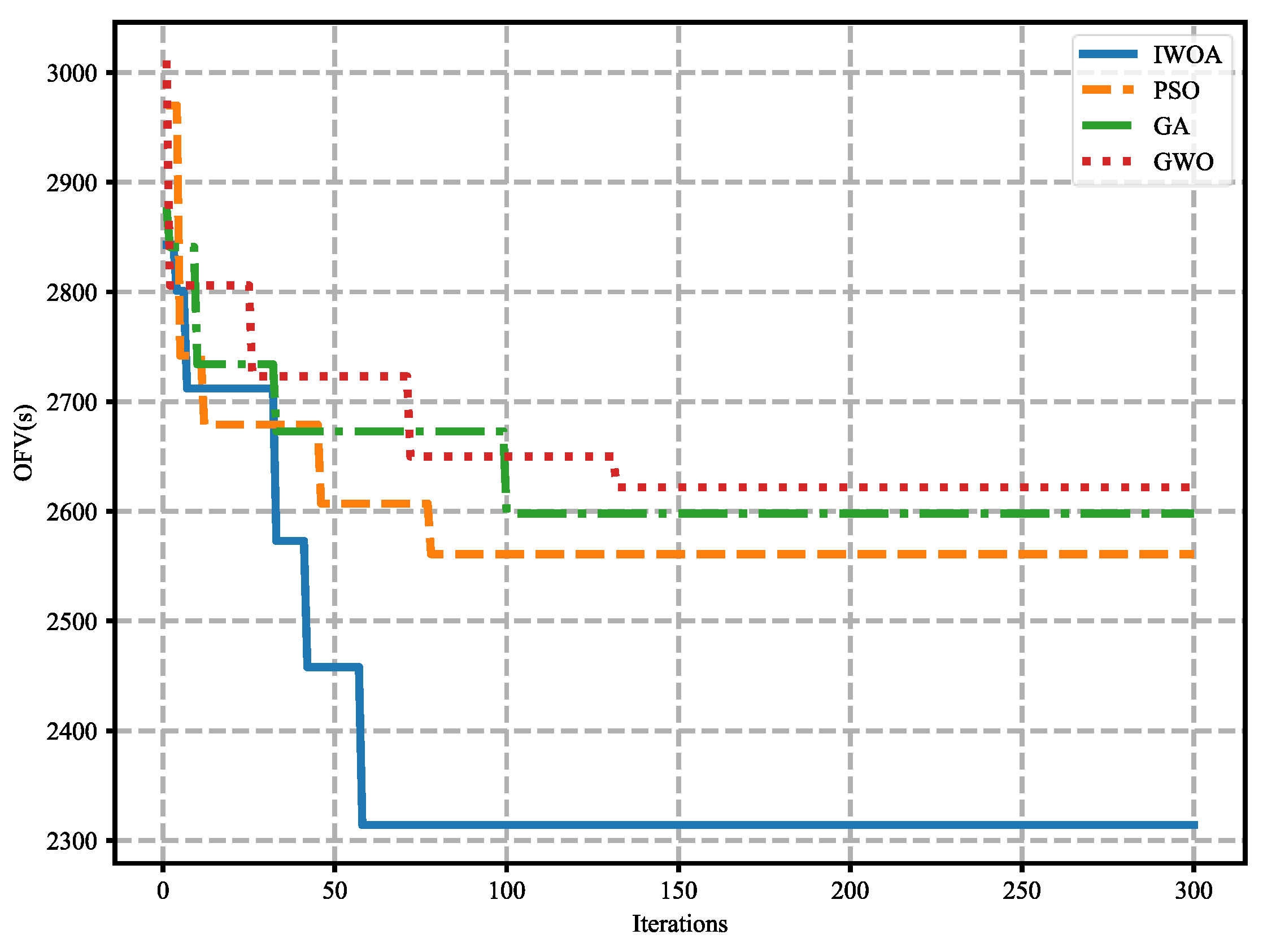
Figure 7 illustrates the convergence rate of each algorithm during the execution of experiment no. 15 in Table 5. The results indicate that the IWOA converges more rapidly, fully validating the effectiveness of the proposed algorithm. Additionally, the high convergence rate of the IWOA enables the results to be obtained within a shorter time frame, which is crucial for enhancing the operational efficiency of the ACTs in practical applications.
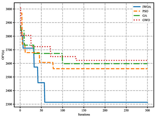
Figure 7.
Algorithm convergence comparison.
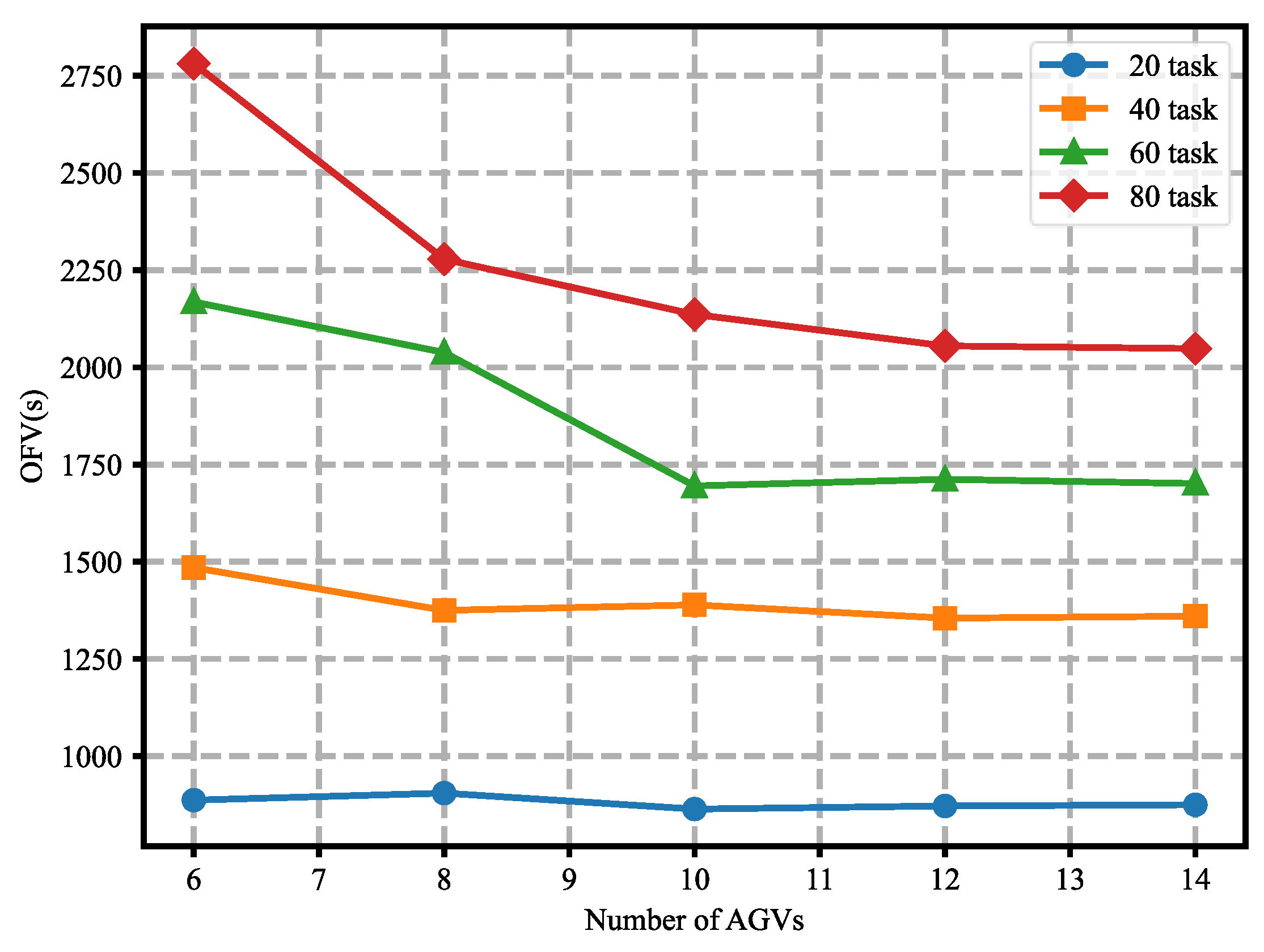
To further evaluate the performance of the developed IWOA solution method under integrated scheduling, the influence of the number of AGVs on the OFV was analyzed. A total of 20 experiments were conducted with varying problem sizes of 20, 40, 60, and 80 tasks (corresponding to 20, 40, 60, and 80 container tasks) and with 6, 8, 10, 12, and 14 AGVs. Figure 8 presents the OFVs obtained using the IWOA with different numbers of AGVs across various problem sizes. The results indicate that increasing the number of AGVs has a negligible impact on the completion time for smaller problem sizes (e.g., 20-task line). However, for larger problem sizes (e.g., 80-task line), an increase in AGVs significantly enhances performance. For the overall scale of the problem, the experimental results show little improvement when increasing the number of AGVs to more than 12. This finding is intuitive because, at some point, the efficiency with which the YC handles container tasks will become bottlenecked, not the AGV.
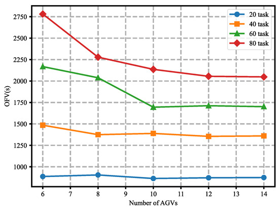
Figure 8.
Effect of the number of AGVs on the OFV.
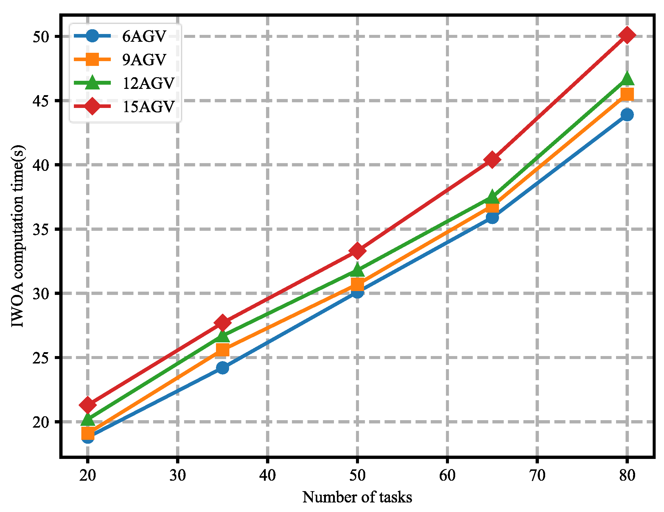
Figure 9 shows the relationship between the computation time of the IWOA and the number of tasks. As expected, as the problem size increases, the computation time for the IWOA also increases. The computation time is more significant with a larger number of AGVs for the same problem size. However, the computation time is not greatly affected by the size of the problem, as quadrupling the problem size (from 20 to 80) does not quadruple the calculation time. These results demonstrate that the developed IWOA method can solve larger YAAISP instances within a reasonable time.
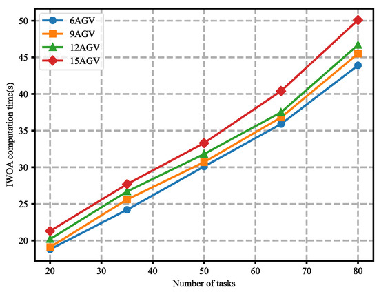
Figure 9.
Effect of the number of tasks on the IWOA’s computation time.
6. Conclusions
This paper investigated the integrated scheduling problem of YCs and AGVs, taking into account the stacking relationships between containers, the bidirectional transportation mode of AGVs, and the road network structure of ACTs. A more comprehensive MIP model was proposed compared to the existing models. The correctness of the model was verified using the CPLEX solver. Since the problem is NP-hard and the CPLEX solver cannot solve it in an effective amount of time with an increase in the problem size, the IWOA was developed. The algorithm introduced population initialization with reverse learning and a random difference mutation strategy to prevent falling into local optima. Additionally, a nonlinear convergence factor and adaptive weighting strategy were employed to dynamically accelerate the search process and improve the convergence speed. Extensive numerical experiments demonstrated the effectiveness of the improved algorithm and its superiority over other algorithms. The models and methods proposed in this study offer quantitative tools for decisionmakers and resource planners to improve the scheduling efficiency of AGVs and YCs. Specifically, these methods can be integrated into terminal operating systems and further refined into decision-support systems tailored for planners in various departments.
In the current study, it is assumed that only one specific size/weight of container was considered. However, it is recognized that containers of different sizes/weights may have a significant impact on loading and unloading processes. In future research, the model will be extended to accommodate various container sizes and explore their effects on scheduling efficiency. Additionally, during the scheduling process of YCs and AGVs, AGV path planning should be considered to prevent collisions or gridlocks in the network. Furthermore, real-time decision-making mechanisms will be integrated to dynamically handle unexpected events, such as equipment failures. These enhancements are expected to further improve the robustness and practicality of the scheduling system, ensuring its applicability in real-world scenarios.
Author Contributions
Conceptualization, S.G. and P.L.; Formal analysis, J.H. and C.F.; Funding acquisition, P.L. and J.H.; Investigation, S.G. and P.L.; Methodology, S.G., P.L. and Y.Z.; Project administration, P.L. and J.H.; Supervision, P.L.; Validation, P.L., J.H. and Y.Z.; Writing—original draft, P.L.; Writing—review and editing, S.G., J.H. and C.F. All authors have read and agreed to the published version of the manuscript.
Funding
This work was supported by the National Natural Science Foundation Committee (NSFC) of China, under grant 52075404, and the National Key Research and Development Project of China, under grant 2020YFB1710804.
Data Availability Statement
The raw data supporting the conclusions of this article will be made available by the authors on request.
Acknowledgments
The authors are grateful to the subjects for their contributions to the experiment.
Conflicts of Interest
The authors declare no conflicts of interest.
Nomenclature
| ACTs | Automated Container Terminals |
| AGVS | Automated Guided Vehicles |
| YCs | Yard Cranes |
| QCs | Quay Cranes |
| YAAISP | Integrated Scheduling Problem of Yard Cranes and Automated Guided Vehicles |
| IWOA | Improved Whale Optimization Algorithm |
| WOA | Whale Optimization Algorithm |
| MIP | Mixed-Integer Programming |
| GA | Genetic Algorithm |
| PSO | Particle Swarm Optimization |
| GWO | Grey Wolf Optimizer |
| OFV | Objective Function Value |
| OFVIS(IWOA) | The OFV obtained by the WOA algorithm under integrated scheduling |
| OFVNIS(IWOA) | The OFV obtained by the IWOA algorithm under non-integrated scheduling |
| OFVIS(WOA) | The OFV obtained by the WOA algorithm under integrated scheduling |
| OFVCPLEX | The OFV obtained by the CPLEX solver under integrated scheduling |
| GAP1 | The difference between the IWOA OFV under non-integrated scheduling and the CPLEX OFV under integrated scheduling |
| GAP2 | The difference rate between the OFV of the IWOA and the CPLEX under integrated scheduling |
| GAP3 | The difference rate between the OFV of the IWOA and the WOA solver under integrated scheduling |
References
- Aslam, S.; Michaelides, M.P.; Herodotou, H. Internet of Ships: A Survey on Architectures, Emerging Applications, and Challenges. IEEE Internet Things J. 2020, 7, 9714–9727. [Google Scholar] [CrossRef]
- Carlo, H.J.; Vis, I.F.A.; Roodbergen, K.J. Storage Yard Operations in Container Terminals: Literature Overview, Trends, and Research Directions. Eur. J. Oper. Res. 2014, 235, 412–430. [Google Scholar] [CrossRef]
- Vanelslander, T.; Sys, C.; Lam, J.S.L.; Ferrari, C.; Roumboutsos, A.; Acciaro, M.; Macário, R.; Giuliano, G. A Serving Innovation Typology: Mapping Port-Related Innovations. Transp. Rev. 2019, 39, 611–629. [Google Scholar] [CrossRef]
- Cao, J.X.; Lee, D.-H.; Chen, J.H.; Shi, Q. The Integrated Yard Truck and Yard Crane Scheduling Problem: Benders’ Decomposition-Based Methods. Transp. Res. Part E Logist. Transp. Rev. 2010, 46, 344–353. [Google Scholar] [CrossRef]
- Mirjalili, S.; Lewis, A. The Whale Optimization Algorithm. Adv. Eng. Softw. 2016, 95, 51–67. [Google Scholar] [CrossRef]
- Song, Y.; Xie, H.; Zhu, Z.; Ji, R. Predicting Energy Consumption of Chiller Plant Using WOA-BiLSTM Hybrid Prediction Model: A Case Study for a Hospital Building. Energy Build. 2023, 300, 113642. [Google Scholar] [CrossRef]
- Hsu, H.-P.; Wang, C.-N.; Thanh Tam Nguyen, T.; Dang, T.-T.; Pan, Y.-J. Hybridizing WOA with PSO for Coordinating Material Handling Equipment in an Automated Container Terminal Considering Energy Consumption. Adv. Eng. Inform. 2024, 60, 102410. [Google Scholar] [CrossRef]
- Shaheen, H.I.; Rashed, G.I.; Yang, B.; Yang, J. Optimal Electric Vehicle Charging and Discharging Scheduling Using Metaheuristic Algorithms: V2G Approach for Cost Reduction and Grid Support. J. Energy Storage 2024, 90, 111816. [Google Scholar] [CrossRef]
- Ng, W.C. Crane Scheduling in Container Yards with Inter-Crane Interference. Eur. J. Oper. Res. 2005, 164, 64–78. [Google Scholar] [CrossRef]
- Saini, S.; Roy, D.; De Koster, R. A Stochastic Model for the Throughput Analysis of Passing Dual Yard Cranes. Comput. Oper. Res. 2017, 87, 40–51. [Google Scholar] [CrossRef]
- Zheng, F.; Man, X.; Chu, F.; Liu, M.; Chu, C. Two Yard Crane Scheduling With Dynamic Processing Time and Interference. IEEE Trans. Intell. Transp. Syst. 2018, 19, 3775–3784. [Google Scholar] [CrossRef]
- Chen, L.; Langevin, A. Multiple Yard Cranes Scheduling for Loading Operations in a Container Terminal. Eng. Optim. 2011, 43, 1205–1221. [Google Scholar] [CrossRef]
- Galle, V.; Barnhart, C.; Jaillet, P. Yard Crane Scheduling for Container Storage, Retrieval, and Relocation. Eur. J. Oper. Res. 2018, 271, 288–316. [Google Scholar] [CrossRef]
- He, J.; Chang, D.; Mi, W.; Yan, W. A Hybrid Parallel Genetic Algorithm for Yard Crane Scheduling. Transp. Res. Part E Logist. Transp. Rev. 2010, 46, 136–155. [Google Scholar] [CrossRef]
- He, J.; Tan, C.; Zhang, Y. Yard Crane Scheduling Problem in a Container Terminal Considering Risk Caused by Uncertainty. Adv. Eng. Inform. 2019, 39, 14–24. [Google Scholar] [CrossRef]
- Li, J.; Yang, J.; Xu, B.; Yin, W.; Yang, Y.; Wu, J.; Zhou, Y.; Shen, Y. A Flexible Scheduling for Twin Yard Cranes at Container Terminals Considering Dynamic Cut-Off Time. J. Mar. Sci. Eng. 2022, 10, 675. [Google Scholar] [CrossRef]
- Liu, W.; Zhu, X.; Wang, L.; Li, S. Flexible Yard Crane Scheduling for Mixed Railway and Road Container Operations in Sea-Rail Intermodal Ports with the Sharing Storage Yard. Transp. Res. Part E Logist. Transp. Rev. 2024, 190, 103714. [Google Scholar] [CrossRef]
- Kim, K.H.; Bae, J.W. A Look-Ahead Dispatching Method for Automated Guided Vehicles in Automated Port Container Terminals. Transp. Sci. 2004, 38, 224–234. [Google Scholar] [CrossRef]
- Rashidi, H.; Tsang, E.P.K. A Complete and an Incomplete Algorithm for Automated Guided Vehicle Scheduling in Container Terminals. Comput. Math. Appl. 2011, 61, 630–641. [Google Scholar] [CrossRef]
- Luo, J.; Wu, Y. Modelling of Dual-Cycle Strategy for Container Storage and Vehicle Scheduling Problems at Automated Container Terminals. Transp. Res. Part E Logist. Transp. Rev. 2015, 79, 49–64. [Google Scholar] [CrossRef]
- Ma, X.; Bian, Y.; Gao, F. An Improved Shuffled Frog Leaping Algorithm for Multiload AGV Dispatching in Automated Container Terminals. Math. Probl. Eng. 2020, 2020, 1260196. [Google Scholar] [CrossRef]
- Angeloudis, P.; Bell, M.G.H. An Uncertainty-Aware AGV Assignment Algorithm for Automated Container Terminals. Transp. Res. Part E Logist. Transp. Rev. 2010, 46, 354–366. [Google Scholar] [CrossRef]
- Xu, W.; Guo, S.; Li, X.; Guo, C.; Wu, R.; Peng, Z. A Dynamic Scheduling Method for Logistics Tasks Oriented to Intelligent Manufacturing Workshop. Math. Probl. Eng. 2019, 2019, 7237459. [Google Scholar] [CrossRef]
- Dang, Q.-V.; Singh, N.; Adan, I.; Martagan, T.; Van De Sande, D. Scheduling Heterogeneous Multi-Load AGVs with Battery Constraints. Comput. Oper. Res. 2021, 136, 105517. [Google Scholar] [CrossRef]
- Zhang, L.; Yan, Y.; Hu, Y.; Ren, W. A Dynamic Scheduling Method for Self-Organized AGVs in Production Logistics Systems. Procedia CIRP 2021, 104, 381–386. [Google Scholar] [CrossRef]
- Li, D.; Tang, J.; Zhou, B.; Cao, P.; Hu, J.; Leung, M.-F.; Wang, Y. Toward Resilient Electric Vehicle Charging Monitoring Systems: Curriculum Guided Multi-Feature Fusion Transformer. IEEE Trans. Intell. Transp. Syst. 2024, 25, 21356–21366. [Google Scholar] [CrossRef]
- Aljanabi, M.R.; Borna, K.; Ghanbari, S.; Obaid, A.J. SVD-Based Adaptive Fuzzy for Generalized Transportation. Alex. Eng. J. 2024, 94, 377–396. [Google Scholar] [CrossRef]
- Shao, Q.; Miao, J.; Liao, P.; Liu, T. Dynamic Scheduling Optimization of Automatic Guide Vehicle for Terminal Delivery under Uncertain Conditions. Appl. Sci. 2024, 14, 8101. [Google Scholar] [CrossRef]
- Zhang, X.; Gu, Y.; Tian, Y. Integrated Optimization of Automated Guided Vehicles and Yard Cranes Considering Charging Constraints. Eng. Optim. 2023, 56, 1748–1766. [Google Scholar] [CrossRef]
- Zhou, C.; Lee, B.K.; Li, H. Integrated Optimization on Yard Crane Scheduling and Vehicle Positioning at Container Yards. Transp. Res. Part E Logist. Transp. Rev. 2020, 138, 101966. [Google Scholar] [CrossRef]
- Zhang, Q.; Hu, W.; Duan, J.; Qin, J. Cooperative Scheduling of AGV and ASC in Automation Container Terminal Relay Operation Mode. Math. Probl. Eng. 2021, 2021, 5764012. [Google Scholar] [CrossRef]
- Chen, X.; He, S.; Zhang, Y.; Tong, L.C.; Shang, P.; Zhou, X. Yard Crane and AGV Scheduling in Automated Container Terminal: A Multi-Robot Task Allocation Framework. Transp. Res. Part C Emerg. Technol. 2020, 114, 241–271. [Google Scholar] [CrossRef]
- Zhang, X.; Li, H.; Sheu, J.-B. Integrated Scheduling Optimization of AGV and Double Yard Cranes in Automated Container Terminals. Transp. Res. Part B Methodol. 2024, 179, 102871. [Google Scholar] [CrossRef]
- Luo, J.; Wu, Y.; Mendes, A.B. Modelling of Integrated Vehicle Scheduling and Container Storage Problems in Unloading Process at an Automated Container Terminal. Comput. Ind. Eng. 2016, 94, 32–44. [Google Scholar] [CrossRef]
- Ma, M.; Yu, F.; Xie, T.; Yang, Y. A Hybrid Speed Optimization Strategy Based Coordinated Scheduling between AGVs and Yard Cranes in U-Shaped Container Terminal. Comput. Ind. Eng. 2024, 198, 110712. [Google Scholar] [CrossRef]
- Zhao, M. An Improved PSO-GWO Algorithm With Chaos and Adaptive Inertial Weight for Robot Path Planning. Front. Neurorobotics 2021, 15, 770361. [Google Scholar]
- Yuan, Q.; Sun, R.; Du, X. Path Planning of Mobile Robots Based on an Improved Particle Swarm Optimization Algorithm. Processes 2022, 11, 26. [Google Scholar] [CrossRef]
Disclaimer/Publisher’s Note: The statements, opinions and data contained in all publications are solely those of the individual author(s) and contributor(s) and not of MDPI and/or the editor(s). MDPI and/or the editor(s) disclaim responsibility for any injury to people or property resulting from any ideas, methods, instructions or products referred to in the content. |
© 2025 by the authors. Licensee MDPI, Basel, Switzerland. This article is an open access article distributed under the terms and conditions of the Creative Commons Attribution (CC BY) license (https://creativecommons.org/licenses/by/4.0/).