Abstract
Given a signed graph and a positive real number r, if there exists a vertex mapping satisfying that for every positive edge , and for every negative edge , or , then admits a circular r-coloring. We use to represent the circular chromatic number of , which is the minimum r, such that a circular r-coloring of exists. This paper proves that , where is a simple signed planar graph containing no cycles of length 4 to 9. Moreover, we establish an upper bound for the chromatic number of such a graph to be .
MSC:
05C15; 05C22
1. Introduction
A graph G is considered to have a proper s-coloring if there is a mapping satisfying that for every edge , the vertices w and x are assigned different colors, which means that . The study of coloring problems on planar graphs can be traced back to the four-color theorem, which asserts that each planar graph has a proper 4-coloring. In 1958, Grötzsch [1] proposed a more specific result: every triangle-free planar graph has proper 3-coloring. Based on the above results, we are devoted to seek sufficient conditions such that planar graphs can be properly colored with, at most, 3 colors. In 1988, Vince [2] introduced the concept of circular coloring, which can be regarded as a refinement of proper coloring of graphs. More results about circular coloring in planar graphs are presented in [2,3].
Recently, Naserasr et al. [4] proposed the concept of circular coloring of signed graphs, which can be viewed as an extension of the concept of circular coloring in graphs. Let be a signed graph that every edge has a mapping .
Definition 1
([4]). Let be a signed graph and be two integers with s being even and . A circular -coloring of is a vertex mapping satisfying that for every edge , when ,
and when ,
The circular chromatic number of is defined as
In [4], Naserasr et al. proposed that each simple signed bipartite planar graph with the maximum degree of all vertices in one partite set being smaller than or equal to 2 satisfies that , which is a rephrased version of the Four-Color Theorem. Furthermore, they showed that when is a simple signed bipartite planar graph, . The upper bound is tight when . Recently, Li et al. [5] provided some results about the circular chromatic number concerning a signed graph with a high girth. The girth of a graph G refers to the length of the shortest cycle of G, and we denote it as .
Theorem 1
([5]). Let be a signed planar graph and k be an integer with .
- (a)
- When , we have .
- (b)
- When , we have .
- (c)
- When , we have .
Thus, we can see that when . Restricted to signed planar graphs, we propose the following result. Here, we mainly focus on considering the chromatic number for a simple signed planar graph containing no cycles of length .
Theorem 2.
For a simple signed planar graph without cycles of length from 4 to 9, the chromatic number is strictly less than 4.
Now, we provide the structure of the rest of this work. Next, we propose some fundamental notations and the concept of circular flows of signed graphs, which is the duality of circular colorings in signed graphs. Then, we introduce some results about the relationship between circular flows and strongly-connected orientations satisfying some boundary conditions. Moreover, using the preparations, we focus on a particular property associated with the wheel graph . In Section 3, we provide the main structural theorem (Theorem 4) of this paper, which we use to prove Theorem 2. Subsequently, to prove Theorem 4, we mainly explore some properties of a minimum counterexample , provide some forbidden configurations of , and utilize the discharging method to derive a contradiction.
2. Preliminary
In this paper, graphs may include multiple edges but no loops. Given a planar graph , let (, or ) represent the number of vertices (edges or faces, respectively). Given a vertex w of G, if (, , respectively), then we call w a t-vertex (-vertex, -vertex, respectively). For a planar graph, an edge e or a vertex w is incident to a face f when e or w lies on the boundary of f. Let and be two faces, if there is at least an edge lying on both and , then we call and adjacent.
For orientation D on a graph G, let and represent the number of edges out from w and into w for each . We call an orientation of a connected graph strongly connected when each edge is in a directed cycle.
In [6], Tutte proposed the dual relationship between integer flows and colorings, which link problems of flows and colorings. Therefore, we have a new perspective on the study of coloring problems. Recently, Li et al. [5] proposed the definition of circular flows of signed graphs, which is the dual concept of circular colorings in the signed graphs studied in [4].
Definition 2
([5]). Let be a signed graph and be two integers with s being even and . A circular -flow in is defined as a pair , where D is an orientation of G and f is a mapping satisfying that for each ,
- (1)
- when , we have ;
- (2)
- when , we have ;
- (3)
- the out-flow of x is equal to the in-flow of x for each .
The circular flow index of is defined as follows:
Thus, in the dual setting, Theorem 2 can be restated that the circular flow index is strictly less than 4 for a signed planar graph that is 3-edge-connected and has no edge-cut with size . Here, we need to mention that if has an edge-cut with size 1 or 2, then the dual graph of contains a loop or multiple edges, which does not satisfy the simple graph condition of Theorem 2. It has been introduced in [7] that circular r-flow of signed graphs with is related to graphs with a special strongly connected orientation. Thus, when proving that , we can transform the problem into seeking a special strongly connected orientation of , as shown in the following theorem. Let represent the number of positive edges that are incident to a vertex w in .
Theorem 3
([7]). Let be a signed graph. If admits a strongly connected orientation D satisfying that for each , , then .
The orientation introduced in Theorem 3 is a specific instance of a strongly connected orientation satisfying some boundary conditions. Now, we introduce the related definitions proposed in [8].
Definition 3
([8]). Given a graph G,
- (i)
- if there exists a function satisfying thatthen β is a parity-compliant -boundary, abbreviated as-pc-boundary.
- (ii)
- An orientation D of G is said to be an -orientation if for every based on a -pc-boundary β of G.
Based on the above definition, we propose two sets of graphs that are frequently used in this paper.
Definition 4.
- (i)
- Let be the set of every connected graph admitting an -orientation, where β is an arbitrary -pc-boundary.
- (ii)
- Let be the set of every connected graph admitting a strongly connected -orientation, where β is an arbitrary -pc-boundary.
For a signed graph , let be a mapping of satisfying that for every . Note that is naturally a -pc-boundary in the graph . Thus, if we prove that , then we can directly obtain the orientation on stated in Theorem 3. In this work, we propose a general result (Theorem 4) about strongly connected orientations with an arbitrary boundary and we prove it in Theorem 3.
Note that contraction and lifting are two useful operations when exploring problems about flows and group connectivity. An operation of contracting an edge means that we identify the vertices w and x, and remove the resulting loop. Furthermore, we refer to the derived graph as , which is formed by contracting all edges of a connected subgraph H of G. Let denote an edge-pair at a vertex x for any two edges . The operation of lifting an edge-pair means that we delete and create a new edge between u and w. Now, we introduce some results related to modifying boundaries when contracting a connected subgraph.
Lemma 1
([9]). Given a graph G and a -pc-boundary β of G, let where H is a connected subgraph of G, and let be the new vertex that results from contraction. We establish a new function , where
Thus, is a -pc-boundary of and we call a corresponding -pc-boundary of .
Lemma 2.
For a graph G, a vertex , and a -pc-boundary β of G, we do some lifting at x to form a new graph . When contains an induced subgraph H which is a member of and has an -orientation , we can extend to obtain an -orientation of G.
Proof.
Let . We define a mapping on as follows,
Note that is a -pc-boundary of H. As , we know that H admits an -orientation . We notice that some edges in H are obtained by doing some lifting at x. Now, we define an orientation based on . For each edge in H formed by lifting at x and oriented from to under , we define a directed path in ; and for the other edges e in H, let . Note that and for each .
Let . We claim that D is an -orientation of G.
- For each , .
- For each , .
- For each , .
Hence, we complete the proof. □
More generally, it has been proved in [10,11] that contraction is preserved with respect to and .
Proposition 1
([10,11]). For a graph G and its connected subgraph , if and belong to (or ), then (or ).
Furthermore, we introduce another set of graphs that can be contractible related to , which is proposed in [11].
Definition 5.
- (i)
- A graph G is a supergraph of a graph H if , and there are two vertices of H satisfying that has a -path.
- (ii)
- Given a graph H, let G be a supergraph of H. Given an arbitrary -pc-boundary β of G and the corresponding -pc-boundary of , we call H weakly contractible with respect to if G can have a strongly-connected -orientation by extending a strongly connected -orientation on .
- (iii)
- We define as the set of all graphs that are weakly contractible with respect to .
According to Definition 5, we know that graphs in have nice “contractible” properties concerning .
Proposition 2
([11]). For a graph G and its connected subgraph , when and , it follows that .
It has been introduced in [11] that graphs in are closed to graphs in .
Lemma 3
([11]). A graph H is in if and only if belongs to , where w and x are two distinct vertices of H.
According to the definition of graphs in , together with Hamiltonian properties, we can easily derive the next lemma.
Lemma 4
([11]). A graph belongs to if it has a Hamiltonian cycle C such that the resulting graph formed by deleting the edges of C belongs to .
Graphs on at most four vertices of are characterized in [9]. Applying the above lemmas, we obtain some graphs belonging to and .
Observation 1.
- [9] Observe that .
- Moreover, .
Now, we begin to prove a property of a wheel , which is a forbidden configuration related to the proof of a structural result (Theorem 4 in Section 3) in this article. By applying the relationship between the graphs in and , we can find more graphs in , such as the graph .
Lemma 5.
The graph .
Proof.
According to Lemma 3, we can finish the proof by verifying that , where are two arbitrary vertices of . Let , where x is the central vertex of and each is on the 10-cycle of .
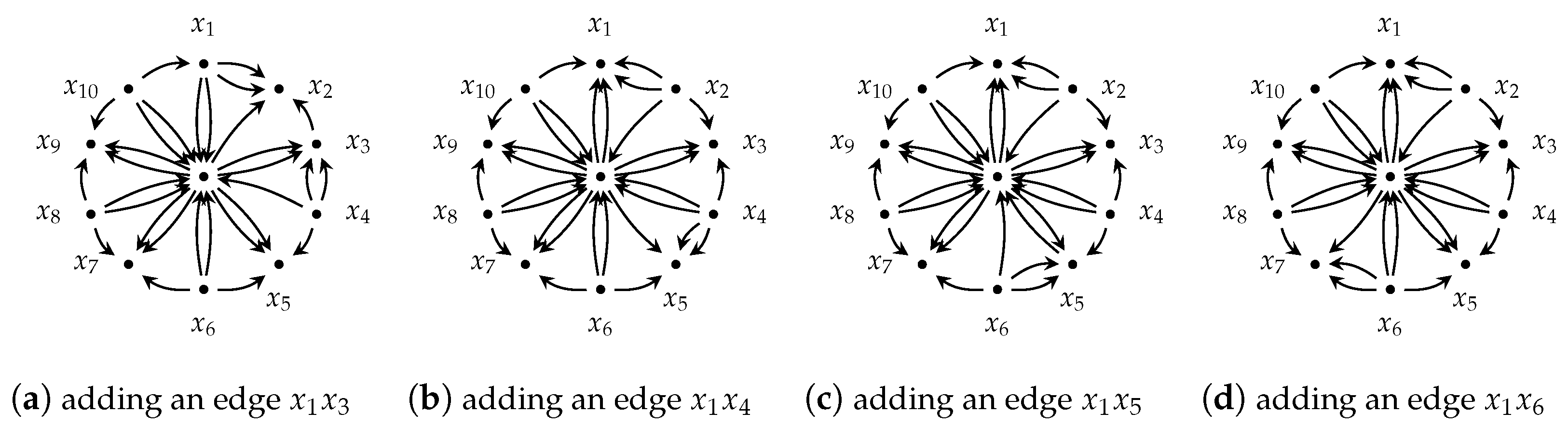
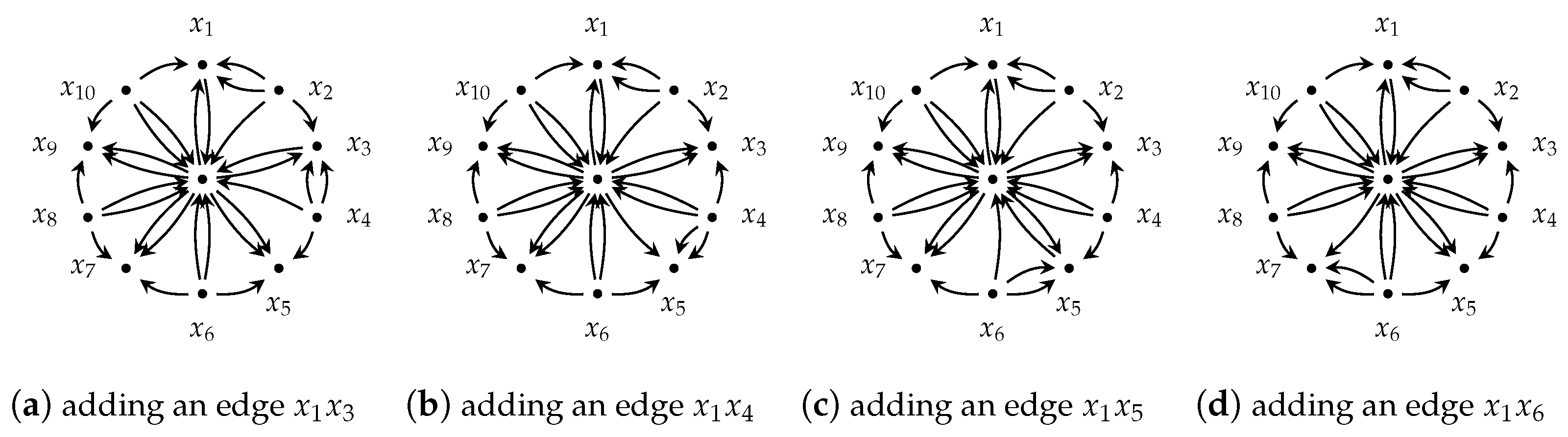
When adding an edge to with w and v being adjacent, we aim to find a Hamiltonian cycle C of , verify that the resulting graph formed from deleting C belongs to , and obtain that by Lemma 4. For the graph with , we choose the Hamiltonian cycle . Let be the resulting graph by deleting this Hamiltonian cycle. Note that contains , which belongs to . Let , and now, there is a in . We denote by the graph formed from contracting a of , where . Note that which belongs to . According to Proposition 1, , and thus by Lemma 4, . For the graph with , we prove that by doing a similar consideration on deleting a Hamiltonian cycle .
Using symmetry, we consider the left cases when adding an edge to with . Now, we still consider the resulting graph formed by deleting a Hamiltonian cycle C of . Here, we choose . Let for every . Note that , , and where . Let be an arbitrary -pc-boundary of .
- When for , we lift an edge-pair , such that there are three parallel edges between x and , and we denote the resulting graph as . We observe that contains belonging to . According to the construction of , there is a sequence of graph , such that each is obtained from by contracting a graph H, where and . Moreover, with the vertex-set , where w is the new vertex formed from contraction. According to Lemma 1, we denote by the corresponding -pc-boundary of . As , we know that , and then . Thus, admits an -orientation. By Lemma 2, admits an -orientation.
- When or , the considerations are similar. Here, we give the proof of the former case. We lift an edge-pair and denote by the resulting graph. Note that . Now, we can obtain a sequence of graphs , such that every is formed from by contracting a graph H, where , , and with the vertex-set . As , we know that , where is a corresponding -pc-boundary of . Note that admits an -orientation. Thus, by Lemma 2, admits an -orientation.
- Now, we consider the left cases that and for . Let denote a triple.
- –
- When , , for , and , we can find an -orientation as depicted in Figure 1.
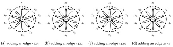 Figure 1. The triple is .
 - –
- When , , for , and , we can find an -orientation as depicted in Figure 2.
 Figure 2. The triple is .
 - –
- When , , for , and , we can find an -orientation as depicted in Figure 3.
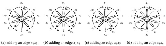 Figure 3. The triple is .
 - –
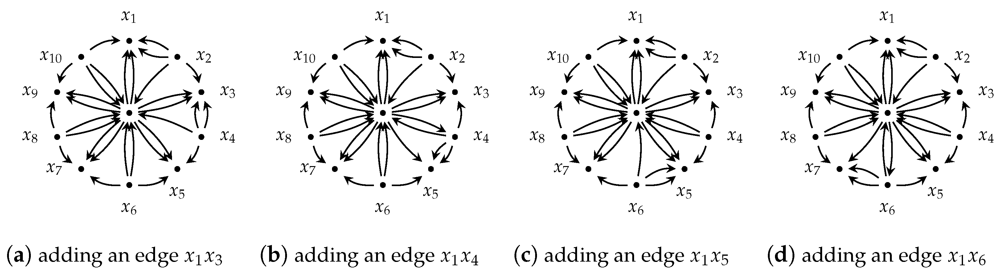
- When , , for , and , we can find an -orientation as depicted in Figure 4.
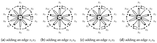 Figure 4. The triple is .
Hence, we know that always has an -orientation for any -pc-boundary , which implies that . According to Lemma 4, for every .
Therefore, we complete the proof. □
3. Main Results
In this section, we are devoted to proving Theorem 4. If Theorem 4 is true, then admits a strongly connected orientation with a special boundary. Together with applying Theorem 3, we can obtain a result of circular flow in a signed planar graph. Considering the duality, we complete to show Theorem 2. When proving Theorem 4, we finish it mainly by contradiction and using the discharging method.
Theorem 4.
For a 3-edge-connected signed planar graph , when G includes no edge-cut with size , we have .
Proof.
Suppose that G is a minimum counterexample with respect to . Thus, . □
Claim 1.
- (i)
- The counterexample G contains no .
- (ii)
- The counterexample G contains no .
Proof.
We prove (i) and (ii) of this claim in the same way. Suppose that G has or as a copy, by analyzing the graph formed from G by contracting or , we will conclude that , which is a contradiction. According to Observation 1 and Lemma 5, we know that . Here, we provide the detailed proof of (i).
If G contains , then . Observe that also meets the condition of Theorem 4, and . Hence, according to the minimality of G. As , together with Proposition 2, we obtain that , which is a contradiction. □
Next, we shall obtain a contradiction of Theorem 4 utilizing the discharging method. We primarily focus on the charges of every vertex and each face in . The condition of Theorem 4 implies that or for each vertex . Before describing our discharging argument, we propose the following easy observation.
Observation 2.
Any two 3-vertices are not adjacent in .
Proof.
It can be obtained by the fact that G has no edge-cut with size .
Discharging part. Initially, we assign a starting charge to every face and vertex. We initialize as for each face , and define for each vertex . Utilizing Euler’s formula, we find that the aggregate charge across all faces and vertices is strictly smaller than 0.
Next, we redistribute the charges of each face and vertex to ensure that they both end with charges that are not negative. Thus, it contradicts the above inequation. Let x be a -vertex and w be a 3-vertex. We call the vertex x semi-poor if is an edge lying on a -face. According to Claim 1(i), we know that G contains no 2-face. Note that only 3-vertex starts with a negative charge. To redistribute charges, we propose the discharging rules as follows.
- Rule (A). Every -vertex gives a charge 1 to its adjacent 3-vertex.
- Rule (B). Every -face sends 1 to its adjacent semi-poor -vertex.
Now, we consider the charge of each face f with . For every 3-face f, it ends with charge . For every -face f, by Observation 2, we know that there are at most 3-vertices incident to f. Thus, there are at most semi-poor -vertices lying on f. According to Rule (B), it ends with charge . Hence, each face finishes with a non-negative charge.
For each 3-vertex w, it starts with . By Observation 2, the vertex w is adjacent with -vertices. By Rule (A), it ends with . For every 10-vertex w, it is incident to at least a -face by the fact that G contains no (Claim 1(ii)). When w is semi-poor, we consider the number of 3-vertices adjacent with w, and denote it as a. When , by Rules (A) and (B), the final charge of w is . If , then w ends with . For every -vertex w, we let m represent the number of 3-vertices adjacent with w. If , then w ends with . If , then w is incident to at least one -face. According to Rules (A) and (B), the vertex w ends with . Thus, every vertex finishes with a non-negative charge.
Therefore, we are done. □
4. Conclusions
In conclusion, we propose the proof of Theorem 2.
Proof of Theorem 2.
Let denote the dual signed planar graph of . Thus, is 3-edge-connected and has no edge-cut with size . According to Theorem 4, we know that , which means that has a strongly connected -orientation satisfying the condition of Theorem 3. Hence, , and thus possesses a circular r-coloring, where . □
Remark 1.
Actually, we can also infer when a signed simple planar graph contains cycles without length from 4 to 9, the circular chromatic number does not exceed , where n is the number of vertices. It has been proposed in Corollary 1.7 of [12] that there exist an integer t and a cycle of length s in , such that . According to Theorem 2, we have . Thus , and then . According to the parity of and , we have . Hence, . Moreover, by the fact that , we have . Note that the sequence is increasing and when n is fixed, the sequence is decreasing. Hence, if n is odd and if n is even.
Funding
This research received no funding.
Data Availability Statement
No new data were created or analyzed in this study.
Conflicts of Interest
The author declares no conflicts of interest.
References
- Grötzsch, H. Zur Theorie der diskreten Gebilde. VII. Ein Dreifarbensatz für dreikreisfreie Netze auf der Kugel. Wiss. Z. Der-Martin-Luther-Univ.-Wittenberg.-Math.-Naturwissenschaftliche Reihe 1958, 8, 109–120. [Google Scholar]
- Vince, A. Star chromatic number. J. Graph Theory 1988, 12, 551–559. [Google Scholar] [CrossRef]
- Zhu, X. Circular chromatic number: A survey. Discret. Math. 2001, 229, 371–410. [Google Scholar] [CrossRef]
- Naserasr, R.; Wang, Z.; Zhu, X. Circular chromatic number of signed graphs. Electron. J. Comb. 2021, 28, P2.44. [Google Scholar] [CrossRef]
- Li, J.; Naserasr, R.; Wang, Z.; Zhu, X. Circular flows in mono-directed signed graphs. J. Graph Theory 2024, 106, 686–710. [Google Scholar] [CrossRef]
- Tutte, W.T. A contribution to the theory of chromatic polynomials. Can. J. Math. 1954, 6, 80–91. [Google Scholar] [CrossRef]
- Cranston, D.W.; Li, J.; Wang, Z.; Wei, C. Planar graphs with homomorphisms to the 9-cycle. arXiv 2024, arXiv:2402.02689. [Google Scholar]
- Li, J.; Wu, Y.; Zhang, C.-Q. Circular flows via extended Tutte orientations. J. Comb. Theory Ser. B 2020, 145, 307–322. [Google Scholar] [CrossRef]
- Li, J.; Shi, Y.; Wang, Z.; Wei, C. Homomorphisms to small negative even cycles. Eur. J. Comb. 2024, 118, 103941. [Google Scholar] [CrossRef]
- Cranston, D.W.; Li, J. Circular flows in planar graphs. Siam J. Discret. Math. 2020, 34, 497–519. [Google Scholar] [CrossRef]
- Han, M.; Lai, H.-J.; Li, J.; Wu, Y. Contractible graphs for flow index less than three. Discret. Math. 2020, 343, 112073. [Google Scholar] [CrossRef]
- Kardoš, F.; Narboni, J.; Naserasr, R.; Wang, Z. Circular (4-ε)-coloring of some classes of signed graphs. Siam J. Discret. Math. 2023, 37, 1198–1211. [Google Scholar] [CrossRef]

Disclaimer/Publisher’s Note: The statements, opinions and data contained in all publications are solely those of the individual author(s) and contributor(s) and not of MDPI and/or the editor(s). MDPI and/or the editor(s) disclaim responsibility for any injury to people or property resulting from any ideas, methods, instructions or products referred to in the content. |
© 2025 by the author. Licensee MDPI, Basel, Switzerland. This article is an open access article distributed under the terms and conditions of the Creative Commons Attribution (CC BY) license (https://creativecommons.org/licenses/by/4.0/).